A Restricted-Complexity Controller with Crone Control-System Design

A Restricted-Complexity Controller with Crone Control-System Design and Closed-Loop Tuning P. Lanusse†, T. Poinot‡, O. Cois†, A. Oustaloup†, J.C. Trigeassou‡ †

LAP - UMR 5131 CNRS - Université Bordeaux 1 – ENSEIRB http://www.lap.u-bordeaux.fr - {lanusse, cois, oustaloup}@lap.u-bordeaux.fr ‡ LAII - UPRES EA 1219 - Université de Poitiers – ESIP http://laii.univ-poitiers.fr - {poinot, trigeassou}@laii.univ-poitiers.fr

Abstract: In the context of the benchmark problem, "Design and optimisation of restricted complexity controllers", related to an active suspension system, this paper presents the design of an initial controller based on the first and third generation Crone methodologies. The high-level parameters of the controller are then fine-tuned using a "tuned in closed-loop" approach. The optimization technique uses the power spectral density of the closed-loop simulation of a residual force to be minimized. This final controller is finally assessed with a real-time implementation. Keywords: Restricted-complexity, Crone design, Fractional controller, Vibration isolation, Tuning in closed-loop

The Crone control-system design has already been applied to many problems, and in particular to the robust control of previously proposed benchmark problems [Cyrot and Landau, 1993, Rey, et al.,1995] where plants have lightlydamped modes. The Crone method has also been applied to vibratory isolation, particularly in the automotive domain [Oustaloup, et al., 1996]. The new benchmark problem proposed by Professor I. D. Landau et al. deals with the control of an active suspension system for vibration isolation, and we have thus applied Crone control.

• input sensitivity function magnitude ≤ 10dB. 10

0

-10

Magnitude (dB)

1 – Introduction

-20

-30

-40

-50

-60 0

The mechanical system is isolated through the input signal u of the active suspension, and disturbed through the signal up (fig. 1): ±1 PRBS signal with a 800 Hz sampling frequency. The objective is to reduce the Power Spectral Density (PSD) of the residual force measured by the output signal y. The transfer function between up and y models the primary path, and the transfer function between u and y models the secondary path. As defined in the first version of the benchmark problem, its control specification is defined mainly by a frequencydomain constraint on the closed-loop PSD of the residual force y. This constraint is defined from the initial PSD of yOL the output y obtained with u = 0. On the closed-loop PSD of y, the objective is: • up to 20 Hz, modification less than 1dB • reduction of the first resonant peak between 20 and 39 Hz, • amplification less than 3dB between 39 and 150 Hz, • between 150 and 220 Hz, magnitude 30 dB less than the first resonant peak, • from 220 Hz, amplification less than 1dB. Fig. 1 shows the initial PSD and the constraint on the closedloop PSD. Further objectives are: • modulus margin ≥ 0.5, • time-delay margin ≥ 1.5ms,

50

100

150

200 f [Hz]

250

300

350

400

Fig. 1 - Initial PSD (....) and constraint on the closed-loop PSD (___)

Even though these specifications are the first to have been set [Landau, et al., 2000], they are compatible with more recent specifications [Landau, et al., 2002] which are simply expressed differently. As the new main topics of the benchmark problem is the design and the optimisation of restricted complexity (loworder) controllers, our proposed solution is inspired both by the simplest (first generation) Crone methodology, and by all that has been done to adapt the third generation Crone methodology to plants with lightly-damped modes. Rather than using a controller order reduction, our approach is based on the direct design of a restricted complexity controller which is tuned using the high-order model of the plant. Section 2 presents the model identification of the plant. Section 3 presents briefly the Crone control-system design methodology. Section 4 presents the design of discrete-time restricted-complexity controller derived from Crone methodology. Then, this controller is tuned using closedloop simulation and implemented on the real system. 2 – Model identification of the secondary path Three dynamic high-order discrete-time models of the secondary path (the plant to be controlled) are identified

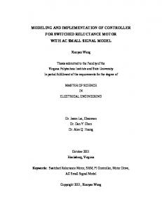
from the 800 Hz sampled experimental data provided successively by the benchmark organisation: the first is an order 16 ARX model with 1 sampling period time-delay; the other two are obtained by minimising an output error (OE) using an order 22 transfer function with 4 sampling period time-delay (parameters [19,15,4] using the System Identification Toolbox [Ljung, 1997] of Matlab). Fig. 2 shows the Bode diagrams of the three frequency responses obtained from the z-domain transfer function of the models and computed using the bilinear w-transform with w= jv = (1-z-1)/(1+z-1). The x-axis unit, v, is the pseudofrequency v as v = tan(ω/2fs), with fs=800Hz here. Magnitude (dB)

40 30 20 10 0 -10 -20 -30 -40

500

Phase (deg)

0

n

 1 + s ωl  CF( s ) = C0  , with ωlωB.  1 + s ωh 

-500

-1000

-1500 -3 10

The constant phase nπ/2 characterizes this controller around frequency ωcg. When the plant corner-frequencies (greatly different from frequency ωcg) or the plant gain vary, the constant phase controller does not modify the phase margin. Thus, the frequency range [ωA, ωB] must at least cover the range where frequency ωcg varies. The first generation Crone strategy is particularly appropriate when the desired open-loop gain crossover frequency ωcg is within a frequency range where the plant frequency response is asymptotic. In this asymptoticbehavior band, the nominal and perturbed plant phases are constant and the plant uncertainty is gain-like. If the plant asymptotic behavior is an order p behavior (p = -2 for second order system), the phase margin Mφ equals (n+p+2)π/2. Around ωcg, the ideal fractional version CF(s) of the controller can also be defined by a band-limited transfer function using corner frequencies:

-2

10

-1

10

0

10

1

10

2

10

Pseudo-Frequency v

Fig. 2 - Bode Diagrams of the three identified plant models

The frequency responses are not so different, but a controller designed that takes the three models into account will be more robust. From v = 0.02, the great phase decrease comes from two left half-plane zeros. These zeros will set an upper limit to the closed-loop frequency bandwidth and will forbid the use of a controller with a high lead effect, which would also provide a gain increase and thus bring instability to the closed-loop system. 3 – Introduction to Crone control-system design Crone control-system design [Oustaloup, et al., 1981, 1999ab, Åström, 1999, Pommier, et al., 2002] is a frequency-domain based design methodology, using fractional differentiation [Miller and Ross, 1993]. It permits the robust control of perturbed plants using the common unity feedback configuration. Three Crone control generations have been developed, successively extending the application fields. The interest of Crone control design is multiple. The use of real or complex fractional differentiation permits the definition of the controller or open-loop transfer function stucture with few high-level parameters. The optimisation problem that provides the optimal values is thus easier to solve. Also, as with QFT [Horowitz, 1993], Crone design takes into account the genuine plant perturbation without over-estimation, so better performance can be obtained by avoiding conservatism [Landau, et al., 1995]. Crone design has already been applied to unstable or non-minimum-phase plants, plants with lightly-damped modes [Lanusse 1994] and discretetime control problems [Oustaloup, et al., 1995]. 3.1 - First generation Crone control-system design The Crone controller is defined within a frequency range [ωA, ωB] around the desired open-loop gain-crossover frequency ωcg from the fractional transfer function of an order n integro-differentiator:

CF( s ) = C0 s n , with n and C0∈ 3.

(2)

(1)

The achievable rational version CR(s) [Oustaloup, 1981, Oustaloup, et al., 2000] of the controller, which can be implemented, is defined by a transfer function resulting from of a recursive distribution of N pairs of real negative zeros and poles: N 1 + s ω' i C R (s ) = C 0 ∏ , (3) + s 1 ω i =1 i with N∈Ð+ and ω'i, ωi ∈ 3+. For the Crone controller to manage the control effort level and steady state errors, the fractional or rational Crone controller has to be complexified. Thus, an order nI bandlimited integrator and an order nF low-pass filter must be included. The complete fractional first generation Crone controller is thus defined by: n

n

ω  I  1 + s ωl  1 , (4) CF(s ) = C0 I + 1   s    1 + s ωh  (1 + s ωF )nF with nI, nF ∈ Ð+, and ωI, ωF ∈ 3+. nF = 0 ensures the constancy of the input sensitivity function, and nF ≥ 1 its decrease. The first generation Crone CSD can be considered as a PID CSD which can adjust independently the value and the frequency range of the derivative lead action. 3.2 - Second and third generation Crone CSD For problems of control effort level (or high input sensitivity function magnitude), it is sometimes impossible to choose an open-loop gain crossover frequency within an asymptotic behavior frequency band of the plant. Thus when the desired ωcg is outside an asymptotic behavior band, the previous Crone controller (1) can not ensure the robustness of the closed-loop system stability margins. Nevertheless, as Bode first stated [Bode, 1945] for the “design of single loop absolutely stable amplifiers” whose tube gains vary, the robust controller is the one which permits the obtention of an open-loop transfer function defined by a constant phase (and dB/oct gain slope) in a useful band. So, when ωcg is within a frequency range where the plant uncertainties are gain-like, the Crone approach defines the open-loop transfer function

(in the frequency range [ωA, ωB] previously defined) by that of a fractional integrator: n

ω  β (s ) =  cg  , with n ∈ 3 and n ∈ [1,2].  s 

(5)

When parameter ωcg varies (consequence of gain-like variations), this definition ensures the robustness of the phase margin Mφ, of the resonant peak Mr (complementary sensitivity function magnitude peak), of the modulus margin Mm, etc. The third generation extends the second by permitting the handling of more general uncertainties than just gain-like perturbations. In a first stage of generalization, the open-loop transfer function (in the frequency range [ωA, ωB] previously defined) is based on the real part (with respect to imaginary unit number i denoted ℜ/ i ) of the fractional complex integration (Oustaloup, et al., 2000): −1  ω  n    p  cg  , β (s ) = cosh  b  ℜ / i  (6)    2 s        with n = a + ib ∈ "i and s = σ + jω ∈ " j . In the Nichols chart at frequency ωcg, the real order a determines the phase placement of the open-loop locus, aπ/2, and then the imaginary order b determines its angle to the vertical. The optimal open-loop positions the open-loop uncertainty domains correctly, so that they overlap the low stability margin areas as little as possible. The minimization of the variations of Mr is carried out under a set of shaping constraints on the four usual sensitivity functions. p

Once the optimal open-loop Nichols locus is obtained, the fractional controller CF(s) is deduced from the ratio of β(s) to the nominal plant function transfer. The design of the achievable controller consists in replacing CF(s) by a rational order controller CR(s) which has the same frequency response: CR ( jω ) = CF( jω ) = β ( jω ) G0( jω ) . (7) 3.3 - Crone control of plants with lightly-damped modes Let G be a plant whose nominal transfer function is: nz  2  ∏ 1 + 2ς zi s + s2  ωnzi ω i =1 nzi  , G0(s ) = Gd(s )  np  2  ∏ 1 + 2ς pi s + s2  ωnp ω  i =1 i npi  

(8)

where: Gd(s) is its well-damped part; the natural frequency and the damping coefficient (ωnzi, ζzi) define one of its nz numerator lightly-damped modes; and the natural frequency and the damping coefficient (ωnpi, ζpi) define one of its np denominator lightly-damped modes. In order to: • avoid the cancellation of some lightly-damped plant modes, • attenuate the peak value of sensitivity functions CS and GS, • attenuate the sensitivity functions T and S at some frequencies, the open-loop transfer function is defined by:

n' z 

s s2  + ∏ 1 + 2ς z i 2 ω nzi ω nz i =1 i β (s ) = β d (s )  n 'p  2 s s  + 2 ∏ 1 + 2ς p i ω np ω np i =1 i i 

  s s2   + 2  n  1 + 2ς 'N i ω ' ω 'nNi nN i  N ∏  i =1 s s2   1 + 2ς N + i 2 ω nNi ω nN   i  

  ,     

(9)

where: βd(s) is defined by (7); n'z ≤ nz and n'p ≤ np are the numbers of uncancelled modes; N(s) is a set of nN notch filters defined by the natural frequencies and the damping coefficients (ω'nNi, ζ'Ni, ωnNi, ζNi). 3.4 – Discrete-time Crone control As part of a Crone control-system design which is a continuous frequency-domain approach, an initial discretetime control-system design problem with the sampling period Ts is transformed into a pseudo-continuous problem by: • taking into account the transfer function of a zero-order hold on the plant input, • computing the z-transform of the continuous set {plant and hold}, • achieving the bilinear variable change z-1 = (1-w)/(1+w). Thus, G(s) becomes successively G0(s) = B0(s)G(s) where B0(s) is the transfer function of the zero-order hold, G0(z) = Z{G0(s)} and G0(w). The controller CF(w) can be designed using the Crone frequency-domain method, given that G0(w) is the frequency response of G0(z) (with z = ejωTs). v is called the pseudofrequency. After the rational synthesis of CR(w), the digital controller C(z-1) is obtained by achieving the inverse variable change w = (1-z-1)/(1+z-1). 4 – Design of the restricted-complexity controller 4.1 - From a Crone controller to the restricted-complexity controller Section 3 shows that the open-loop transfer function has to include the lightly-damped modes of the plant. As these poles will not be included implicitely in the controller, the control-system is able to damp the effect of a disturbance acting on the plant input. Furthermore, to improve the damping of the first lightly-damped modes, it is possible to include in the open-loop several notch filters which can be either amplifiers and/or attenuators. As one main objective of the benchmark problem is the design of a restricted-complexity controller, and as the plant can be modeled by three high-complexity but very closed transfer functions (no great robustness problems), we only need to design a first generation Crone-controller. Even if we used second or third generation Crone-system design: • the controller order would never exceed 9 as it results from a frequency-domain system-identification over a limited frequency range, and does not result from the complexity of an augmented plant (plant plus weighting functions), • the problematic zeros and poles of the plant would not be cancelled by the controller. The use of the first generation Crone-system design, however, avoids the need to cancel many other plant zeros and poles, thus permitting the design of a restrictedcomplexity controller. To damp the system more, the transfer function of the controller includes two notch filters

around its two first lightly-damped pole-pairs whose frequencies are close to 33Hz (v = 0.13) and 160Hz (v = 0.72). The controller is designed using a pseudo-continuous frequency-domain approach as presented in section 3.7. It is defined by the w-domain transfer function: n  1+ w vl v  I C(w) = C0 I + 1  w  1+ w vh  2 w + 2ς'1 vn1w + vn1 2 2 w + 2ς1vn1w + vn1 2

n

  1  n  1 + w  F .    vF   2 w2 + 2ς'2 vn2w + vn2 2 2 w + 2ς 2vn2w + vn2

(10)

As there is no accuracy specification, nI is set to 0. As the closed-loop system needs roll-off, nF is set to 2. To reduce the final controller complexity, vI and vF are set respectively to vl and vh. Thus, the controller to be designed is defined by: C ( w) = C0

1 + w   vl   1 + w   vF  

n

n+2

2 2 w2 + 2ς '1 vn1w + vn1 w2 + 2ς '2 vn2 w + vn2 . (11) 2 2 2 2 w + 2ς1vn1w + vn1 w + 2ς 2vn2 w + vn2

The design of the controller takes into account: • the three identified models of the plant • the required modulus margin • the maximum value of the input sensitivity function • the difference (in dB) between the constraint on the closedloop PSD and the initial PSD of the residual force over a critical frequency range [0Hz, 150Hz].

between the PSD constraint P0 defined by the specification and the PSD POL of yOL. Within the frequency range [0Hz, 150Hz], the difference is weak. The use of the simple first generation Crone methodology needs to set the nominal phase margin and gain crossover frequency, and the corner frequencies vl and vh. The phase margin is set to 75° and vcg is set to 0.14. They are 8 independent high-level parameters. The low and high corner frequencies of the fractional effect of the controller are defined by vl = vcg/5 and vh = vcg*4, namely: vl = 0.0283 and vh = 0.55. The notch parameters are determined by taking into account the simplified constraint S0. A quick tuning leads to vn1 = 0.13, ζ'1 = 0.3, ζ1 = 0.7, vn2 = 0.6, ζ'2 = 0.2, and ζ2 = 0.6. Then, the phase margin and the gaincrossover frequency are ensured with order n = -1.02 and finally gain C0 = 2.4. As n is very close to -1, for this control problem, the performance, and in particular the phase margin, is almost the same when including a rational effect (n = -1) in the controller rather than a fractional one (n = -1.02). Furthermore, chosing n = -1 avoids the need to synthesise the fractional part by a set of zero-pole cells which would increase the controller complexity. So, as we take n = -1, this leads to C0 = 2.3. The time-delay margin measured at v = 0.751 (ω = 1031 rad/s) equals 2.37ms and is greater than the required minimum of 1.5ms.

where G(s) is one of the transfer functions that models the plant (secondary path) and S(s) the common sensitivity function. The PSD as it is computed in the benchmark problem proportional to the Fourier transform of the signal, a constraint P0 on the PSD Py of closed-loop signal y, can be translated as a constraint S0 on S while taking in account the PSD POL of yOL: Py(ω ) P (ω ) S ( jω ) = ≤ 0 = S0(ω ) . (13) POL(ω ) POL(ω ) 20

Magnitude (dB)

15

10

5

0

Magnitude (dB)

5

In the "open-loop" configuration (u = 0), the measured output is yOL. In closed-loop, the transfer from YOL(p) to Y(p) is defined by: Y (s ) 1 = = S(s ) , (12) YOL(s ) 1 + G(s )C(s )

0

-5

-10 -3 10

-2

10

-1

10

0

10

1

10

2

10

Pseudo-frequency v ___

Fig. 4 – Sensitivity function S ( ) for the 3 plant models and simplified constraint S0 (- - -)

Fig. 4 shows that the greatest value of S is around 4.7dB. So, the modulus margin equals 0.58 and is greater than the 0.5 minimum required. Nevertheless, and whatever the plant model taken into account, the sensitivity function S exceeds the minimum constraint S0 around the required attenuation peak. nI = 0 allows respect of the constraint on the greatest value of the input sensitivity function CS over the low frequencies. The greatest value of CS equals 7.9dB and is lower than the 10dB constraint.

-5

-10 0

50

100

150

200

250

300

350

400

f (Hz)

Fig. 3 - Difference between P0 and POL (....); simplified constraint S0 (- -)

Fig. 3 presents a simplified version of constraint S0 defined by seven points {(0.3,1), (18.3,1), (20,0), (31.25,-6.6), (39,0), (42.52,3), (150,3)}, and compares it to the difference

The discrete-time controller with fs = 800Hz is defined by the z-domain transfer function: 6 5 4 3 2 .(17) C( z ) = 0.01106z − 0.01038z − 0.005959z + 0.02425z − 0.01689z − 0.01211z + 0.01355 z6 − 3.491z5 + 5.074z4 − 4.039z3 + 1.919z2 − 0.5207z + 0.05878

At each sampling time, the control-system of fig. 5 requires 13 products and 12 sums.

y

u -

C(z)

+

G(z)

yOL

Fig. 5 – Block diagram used for time-domain simulation

appears to be the increase of vl (and thus the decrease of C0), the fine tuning of the other parameters is also really important. Fig. 7 compares the PSD Py of the simulated closed-loop residual force y, with the PSD POL of the initial open-loop residual force yOL, and with the constraint P0. 0

0

-10

-20

Magnitude (dB)

Magnitude (dB)

-10

-30

-40

-50

-20

-30

-40

-50

-60 0

50

100

150

200

250

300

350

-60

400

f (Hz)

0

50

100

150

200

250

300

350

400

f (Hz)

__ Fig. 6 – Constraint P0 ( ) and PSD of the residual forces: (....) open-loop residual force yOL, simulated closed-loop residual force y (- - -)

Using the matlab-code provided by the Hutchinson company (through the organization), the PSD Py of the simulated closed-loop residual force y is compared with the PSD POL of the initial open-loop residual force yOL, and with the constraint P0 (Fig. 6). As in Fig. 8 which shows that the sensitivity function S exceeds the constraint S0, Fig. 6 also shows that the PSD Py of the simulated y exceeds the PSD constraint P0: over the frequency range [30Hz, 60Hz], the overshoot is about 1 dB. So, this controller has to be improved.

__ Fig. 7 – Constraint P0 ( ) and PSD of the residual forces: (....) open-loop residual force yOL, simulated closed-loop residual force y (- - -)

Fig. 7 shows that the PSD constraint is now respected when using the optimized controller. The optimal discrete-time controller is defined by: 6 5 z 4 + 0.02713z3 − 0.01414z 2 − 0.01393z + 0.01308 C( z ) = 0.01469z −6 0.0093435z − 0.009779 z − 2.797z + 3.223z 4 − 2.023z3 + 0.7469z 2 − 0.1489z + 0.01087

.

(16) Fig. 8 shows the new open-loop Nichols plot for the three plant models. 40

(

)

J = ∫ g Py( f ), P0( f ) df , 0

with the g function:

(

(14)

20

3 dB 6 dB -3 dB -6 dB

10 0 -10

-12 dB

-20

-20 dB

-30

-40 dB

-40 -50 -60 -1800

-1600

-1400

-1200 -1000

-800

-600

-400

-200

0

200

Open-Loop Phase (deg)

) (

g Py( f ), P0( f )

)

 P ( f ) − P0( f ) 2 si Py( f ) > P0( f ) , (15) = y 0 si Py( f ) < P0( f ) 

where Py(f) is the PSD of the simulated residual force and where P0(f) defines the PSD constraint. Outside the frequency range [0Hz, 200Hz], the roll-off makes the control-loop open and the optimization does not have a significant effect. The parameter values of the previous quickly "optimized" controller are used as initial values. During the optimization, the corner-frequencies and the gain can vary up to a factor of 5 (0.2x0 ≤ x ≤ 5x0) and the damping ratios are allowed to vary between ±0.05 and ±2 but without changing their initial sign. The optimal parameters are: vl = 0.137, vh = 0.743, vn1 = 0.180, ζ'1 = 0.464, ζ1 = 1.186, vn2 = 0.610, ζ'2 = -0.118, ζ2 = 0.698, and C0 = 0.630. Even if the main modification

Fig. 8 – Open-loop Nichols plot for the 3 plant models

The first gain-crossover pseudo frequency is vcg = 0.141 with a phase margin about 90°. The time-delay margin measured at v = 0.76 (ω = 1040 rad/s) is 2.3ms. (>1.5ms). 4

2

0

Magnitude (dB)

200

0 dB 0.25 dB 0.5 dB 1 dB -1 dB

30

Open-Loop Gain (dB)

4.2 – Closed-loop tuning of the restricted-complexity controller The previous controller is now tuned using a "tuned in closed-loop" approach. As the real system is not easily available, it is replaced by its model. The closed-loop model used for time-simulation is now used for the optimization of the controller parameters. The optimisation criterion to be minimized measures the overshoot of the PSD constraint P0 over the frequency range [0Hz, 200Hz] by the simulated PSD Py. It is defined by:

-2

-4

-6

-8

-10 -3 10

-2

10

-1

10

10

0

Pseudo-frequency v

10

1

10

2

Fig. 9 – Sensitivity function S (___) for the 3 plant models, and simplified constraint S0 (- - -)

Fig. 9 shows that the simplified constraint S0 on the sensitivity function S (for the three plant models) is now almost completely respected. The greatest value of S is around 3.37dB. So, the modulus margin is 0.68 (>0.5). The greatest value of CS is -3.95dB (