A Rigorous, Compositional, and Extensible Framework for Dynamic

This article has been accepted for publication in a future issue of this journal, but has not been fully edited. Content may change prior to final publication. IEEE TRANSACTIONS ON DEPEDABLE AND SECURE COMPUTING 1

A Rigorous, Compositional, and Extensible Framework for Dynamic Fault Tree Analysis Hichem Boudali, Member, IEEE, Pepijn Crouzen, and Mariëlle Stoelinga

Abstract— Fault trees (FT) are among the most prominent formalisms for reliability analysis of technical systems. Dynamic FTs extend FTs with support for expressing dynamic dependencies among components. The standard analysis vehicle for DFTs is state-based, and treats the model as a CTMC, a continuous-time Markov chain. This is not always possible, as we will explain, since some DFTs allow multiple interpretations. This paper introduces a rigorous semantic interpretation of DFTs. The semantics is defined in such a way that the semantics of a composite DFT arises in a transparent manner from the semantics of its components. This not only eases the understanding of how the FT building blocks interact. It also is a key to alleviate the state explosion problem. By lifting a classical aggregation strategy to our setting, we can exploit the DFT structure to build the smallest possible Markov chain representation of the system. The semantics - as well as the aggregation and analysis engine is implemented in a tool, called CORAL. We show by a number of realistic and complex systems that this methodology achieves drastic reductions in the state space. Index Terms— Fault trees, Reliability, Compositionality, Formal models, Framework.

I. I NTRODUCTION ELIABILITY ENGINEERING is an important activity in the design of today’s computer and communication systems. For safety critical systems, such as airplanes and nuclear power plants, failures can be life threatening; for other applications, such as online ticket vending systems, failures often incur a high cost. One of the most popular formalisms to model and analyze systems’ reliability is the fault tree (FT) formalism [27]. Dynamic fault trees (DFT) [13], [8], [26] extend standard (or static) FTs by defining additional gates called dynamic gates. These gates allow the modeling of complex system components’ behaviors and interactions which greatly increases the modeling capabilities of standard FTs. Like standard FTs, dynamic fault trees are a high-level formalism for computing reliability measures of computer-based systems. For over a decade now, DFTs have been experiencing a growing success among reliability engineers. DFTs, like FTs, describe the system failure in terms of the failure of its components. A DFT is a tree (or rather a directed acyclic graph (DAG), since subtrees can be shared) in which the leaves are basic events (BEs) and the other elements are gates. A BE typically models the failure of a physical component and is governed by a probability distribution. In this paper, we consider exponential distributions and phase-type distributions, the latter allowing to approximate other probability distributions with arbitrary precision. Gates express how component failures induce system failures and are either static (AND, OR, and the

R

This research has been partially funded by the Netherlands Organisation for Scientific Research (NWO) under FOCUS/BRICKS grant number 642.000.505 (MOQS); the EU under grant IST-004527 (ARTIST2) and FP7ICT-2007-1 grant 214755 (QUASIMODO); and by the DFG/NWO bilateral cooperation programme under project number DN 62-600 (VOSS2)

Digital Object Indentifier 10.1109/TDSC.2009.45

K/M voting gate) or dynamic (Priority AND, SPARE, and the Functional Dependency gate). DFTs are typically used to compute system unreliability, that is, the probability that the system fails during a specified period of time (usually called mission time) and under given conditions. Other measures, such as the average time until a failure occurs can be computed as well. Despite their success, current DFT analysis methods have several (mutually related) drawbacks. 1) Existing analysis methods (most notably, the DIFTree method [21] implemented in analysis tools like Galileo [25] and Relex [23]) typically convert a DFT into a continuoustime Markov chain (CTMC) whose states are vectors of modes (up, failed, active, inactive) for each BE. Hence, the size of the state space is exponential in the number of basic events. 2) These methods impose rather severe syntactic restrictions on DFTs, greatly diminishing the modeling flexibility and power of DFTs. Most notably, DFT spare components must be BEs, whereas spare components in practice are often entire subsystems. 3) The DFT semantics is rather imprecise and the lack of formality has, in some cases, led to undefined behavior and misinterpretation of the DFT model. 4) DFTs lack comprehensive modular analysis. DIFTree uses a limited form of compositional analysis: it solves in a separate way all stochastically independent subtrees of a static gate, provided none of its ancestors in the tree is a dynamic gate. Then it combines, using Binary Decision Diagrams, their analysis results to obtain the result for the entire DFT. However, this method is not applicable to dynamic gates. In particular, those DFTs whose top-node is a dynamic gate can not be analyzed compositionally. 5) The current methods are difficult to extend or to modify. In this paper, we present a framework for DFT analysis based on I/O-IMCs that greatly alleviates these drawbacks. I/O-IMCs are a powerful and versatile formalism to model and analyze stochastic system behavior, and have been used in an number of applications, ranging from telecommunication systems [18] to railway networks [3] and multiprocessor arrays [11]. I/O-IMCs extend CTMCs with input, output and internal actions, used for communication between several I/O-IMCs. They are equipped with a parallel composition operator, allowing one to build larger I/O-IMCs from smaller ones, and with powerful minimization (a.k.a. lumping) techniques to reduce the state space of an I/OIMC. The core of our methodology is a compositional semantics of DFTs in terms of I/O-IMCs. That is, we translate each DFT element (i.e. gate or BE) into one or more I/O-IMCs — obtaining these semantics turned out to be non-trivial, and required a careful re-examination and generalization of the concept of spare

1545-5971/09/$26.00 © 2009 IEEE


activation. Then, the semantics of an entire DFT is obtained as the parallel composition of all DFT element I/O-IMCs. Since these I/O-IMCs semantics pin down the meaning of a DFT in a mathematically precise way, we lift drawback 3 mentioned above. Relatedly [10] presented a formal semantics in Z. The main difference between the formal specification in [10] and the formal specification used in this paper is that in our framework we use a process algebra-like formalism (i.e. I/O-IMC) which comes with two very powerful concepts, namely parallel composition and aggregation/minimization. Since composing all element I/O-IMCs at once would give the same blow up as the DIFTree method, we use the compositional aggregation method to reduce the size of the models. That is, we compose two I/O-IMCs, hide actions that are no longer needed for communication with other components, and minimize them. We repeat this process until all element I/O-IMCs have been composed. While this method is still exponential in worst case, our experiments show that serious reductions (one or two orders of magnitude) are realized in practice. Thus, our methodology relieves drawback 1 mentioned above. Since this analysis method is fully compositional, that is, the analysis of a DFT (i.e. its underlying I/O-IMC) is obtained from analysis results of its components (i.e. lumped I/O-IMCs of sub-models), we also lift drawback 4. We note that the order in which we compose these I/O-IMCs matters for the size of the intermediate I/O-IMC models, but not for the final result. We employ heuristics, based on the way individual I/O-IMC models communicate with each other, to obtain smart composition orders. These models have specific properties (acyclicity) that we exploit by tailored algorithms. Also, it turns out that our techniques require much lighter syntactic restrictions than existing DFT methodologies. Any subsystem can now be used as a dependent event and any activation-independent (see Section IV) can be used as a spare component. Hence, drawback 2 is alleviated. Finally, we show how the current DFT semantics can readily be extended or modified; we present extensions with inhibition, mutual exclusion and repair, thus addressing drawback 5. We have implemented our DFT framework in a tool called CORAL. The tool derives all I/O-IMC models and composes them using the CADP tool-set [15], which is also used to compute the system reliability. We used CORAL to analyze nine case studies, including ones showing systems with spare and dependent event subsystems which are currently not supported by any other DFT tool and a system showing the need for non-determinism. We have compared our tool with Galileo and our experiments show that, in almost all cases, our tool is much faster and generates significantly smaller models (where we consider the largest model encountered during analysis). This paper combines and extends the work previously carried out in [7] and [5]. In particular, our contributions over these papers are 1) a complete semantics of all DFT elements: Whereas [7] and [5] describe the semantics of DFT gates for a specific number of inputs, we cover here the general case, employing the IOIML notation. Moreover, we allow phase-type distributions as failure distributions of basic events; 2) a complete proof for the congruence theorem; 3) a more extensive set of case studies including systems with spare and dependent event subsystems which are not

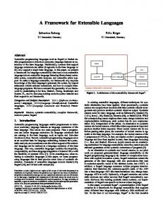
currently supported by any other DFT tool and examples showing the need of non-determinism; 4) CORAL, our prototype tool for analyzing DFT using the I/O-IMC semantics. It employs the specialized I/O-IMC minimization algorithm from [12], yielding much faster computation times than [7] and [5]. a) Organization of the paper.: The remainder of the paper is organized as follows: In Section II we introduce DFTs and in Section III we discuss I/O-IMCs. In Sections IV and V we present the formal DFT syntax and semantics respectively. In Section VI, we show, through three examples, how one can readily extend the existing DFT formalism. Section VII presents the compositional aggregation technique and Section VIII describes the CORAL tool. Finally, in Section IX, we present a number of case studies and Section X concludes the paper. II. DYNAMIC FAULT TREES As described in Section I, DFTs and FTs are directed acyclic graphs describing the system failure in terms of the failure of its components. Their leaves are labeled with basic events, and non-leaves with gates. 1) BE: A BE, graphically depicted by a circle (see Figure 1(g)), typically represents the failure of a basic system component; its failure behavior is governed by a probability distribution. In order to describe these distributions using I/OIMCs, this paper considers exponential and (acyclic) phase-type distributions, the latter allowing to approximate other probability distributions with arbitrary precision. An exponential distribution has a parameter λ that represents the component’s failure rate (i.e. number of failures per time unit). A BE has three modes of operation: dormant, active, and failed. In dormant (or standby) mode, the BE failure rate λ is reduced by a factor α ∈ [0, 1] called dormancy factor. Thus, the BE failure rate in standby mode is μ = αλ. In active mode, the failure rate is unchanged and equals to λ. The dormancy is relevant when the BE is used as a spare (more details on spare BEs is provided below). In failed mode, the BE, as the name suggests, has failed and remains in that state (i.e. we do not consider repairable systems at this point). Phase-type basic events (PHBE) are basic events that fail after a delay governed by a phase-type (PH) distribution [22] with a finite number of phases. The passive behavior of a PHBE is also described by a PH distribution with a finite number of phases. Activation of a PHBE is described by a function which links passive phases to active phases. When a PHBE is activated it moves from its current passive phase to the associated active phase. Note that a BE (with exponential distribution) is a special case of a PHBE where both active and passive distributions have only one phase. 2) Gates: Non-leaf elements are called gates and express how component failures induce system failures. Their graphical representation is given in Figures 1(a)-(f). Each gate has one or more inputs, corresponding to outputs of other elements, and exactly one output. It often represents or maps to a subsystem contained in the whole system, the top element representing the system failure. When the failure event of a BE or a gate occurs, we use the terms failing, occurring, or firing interchangeably. Gates can either be static (AND, OR gate, and VOTING (also called K/M) gate) or dynamic. Static gates (which are the only gates in static fault trees) are combinatorial: they are only sensitive


to the combinations of failures of their inputs and not to their order. Dynamic gates allow the modeling of sequence dependencies (via the priority AND (PAND) gate), functional dependencies (functional dependency (FDEP) gate) and spare management and allocation (via the SPARE gate)1 . Thus, DFTs enrich the FT formalism with powerful and yet easy-to-use modeling capabilities. Below, we describe all DFT gates. output

output

output

Road trip fails

2/3 inputs inputs inputs (a) AND gate (b) OR gate (c) VOTING gate output

Tires fail output

dummy output

trigger primary inputs event dependent events tire spares (d) PAND gate (e) SPARE gate (f) FDEP gate

Fig. 1.

Car fails phone

engine

a cold spare and can not by definition fail before the primary. When α = 1, the spare is called a hot spare and its failure rate is the same whether in standby or in active mode. If 0 < α < 1, the spare is called a warm spare. Example 1 Figure 1(g) shows a DFT modeling a road trip. Looking at the top PAND gate, we see that the road trip fails (i.e. we are stuck on the road) if the car fails after the mobile phone has failed; if the car fails first, then we can call the road services to tow the car and continue our journey. The car subsystem fails if either the engine fails or the tires subsystem fails. The car is equipped with a spare tire, which can be used to replace any of the primary tires; when a second tire fails, the tires subsystem fails, causing in turn a car failure. Thus, we model the tires subsystem by four spare gates, each having a primary tire and all sharing a spare tire. The spare tire is a cold spare, i.e. its failure rate is zero in standby mode. A. Simultaneity and non-determinism

tire

tire

tire

spare

(g) DFT example

DFT gates and example.

3) AND gate: The AND gate fails when all of its inputs fail. 4) OR gate: The OR gate fails when at least one of its inputs fails. 5) VOTING gate: A K/M VOTING gate fails when at least K (called the threshold) out of its M inputs fail. 6) PAND gate: The PAND gate fails when all its inputs fail and fail from left to right (as depicted in the figure) order. 7) FDEP gate: The functional dependency gate consists of a trigger event (i.e. a failure event) and a set of dependent events. When the trigger event occurs, it causes all the dependent components to become inaccessible or unusable. Essentially, once a dependent component is triggered, it is assumed to have failed. Dependent events, as originally defined in [13], need to be BEs. This restriction will be later lifted in our framework. All dependent events and the trigger event are considered to be inputs to the FDEP gate. The FDEP gate’s output is a ‘dummy’ output (i.e. it is not taken into account during the calculation of the system failure probability). 8) SPARE gate: The SPARE gate has one primary input and zero (which is a degenerated case) or more alternate inputs called spares. The primary input of a SPARE gate is initially powered on (i.e. in active mode) and the alternate inputs are in standby mode. When the primary fails, it is replaced by the first available alternate input (which then switches from standby mode to active mode). This operation is called spare activation and causes the spare to switch from dormant to active mode. In turn, when this alternate input fails, it is replaced by the next available alternate input, and so on and so forth. Note that multiple spare gates can share a pool of spares. When the primary unit of any of the spare gates fails, it is replaced by the first available (i.e. not failed or not already taken by another spare gate) spare unit; which becomes, in turn, the active unit for that spare gate. The SPARE gate fails when the primary fails and all its spares are failed or unavailable. If all SPARE inputs are BEs, two special cases arise depending on the spare’s dormancy factor α. If α = 0, the spare is called 1 A fourth gate called ‘Sequence Enforcing’ gate introduced in[13] can be emulated using a cold spare gate.

In earlier development of the DFT modeling formalism, the semantics (i.e. the model interpretation) of some DFT configurations, where FDEP gates are used, remained unclear. For instance, in Figure 2, the FDEP gate triggers (in both configurations) the failures of two basic events. Does this mean that the dependent events fail simultaneously and if so what is the state of the PAND gate in the left configuration and which spare gate gets the shared spare S in the right configuration? These examples were also discussed in [10], and we believe that this is an inherent nondeterminism in these models. Whereas in [10], these special cases are dealt with by systematically removing the non-determinism by transforming it into a probabilistic (or deterministic) choice. In our framework, we allow non-determinism should this be intentional or unintentional. If the non-determinism was not intended, then its presence (which is easily detected) indicates that an error occurred during the model specification. Non-determinism could also be an inherent characteristic of the system being analyzed, and should therefore be explicitly modeled.

T Fig. 2.

A

B

T

A

S

B

The occurrence of non-determinism.

In the I/O-IMC formalism, the DFT configurations depicted in Figure 2 will be interpreted as follows: Whenever the dependent events failure has been triggered, then the trigger event (the cause) happened first and was then immediately (with no time elapsing) followed by the failure of the dependent events (the effect). This adheres to the classical notion of causality. Moreover, the dependent events fail in a non-deterministic order (i.e. essentially considering all combinations of ordering). In this case, the final I/O-IMC model is not a continuous-time Markov chain but rather a continuous-time Markov decision process (CTMDP), which can be analyzed by computing bounds of the performance measure of interest [2]. As an example, we have modeled and analyzed a simple non-deterministic case study (see Subsection IX) using the MRMC model-checker [19]. However, the conversion of I/OIMCs to CTMDPs, which closely follows [17], has not yet been automated in the tool-chain.


B. Lifting DFT restrictions Previously, DFT required all inputs to a SPARE gate and all dependent events of an FDEP gate to be basic events. This restriction greatly diminishes the modeling power of DFTs, since it is very natural to have spare components that are comprised of multiple components or subsystems. To lift this restriction, we need to carefully reexamine the notion of spare activation. For primaries and spares that are complex systems, we say that a BE b is a primary-BE (or just primary) of a SPARE gate G if b is contained in the subtree that constitutes the primary of G. This is the case if there exists a path from b to G whose last edge ends in the first input of G. Spare-BEs are defined analogously. The basic idea behind spare activation is that all BEs that are primary-BEs of some SPARE gate are activated from the beginning. A BE that is a spare-BE of some SPARE gate gets activated as soon as one of its SPARE parents is activated. Since spares can be shared, a BE can have multiple SPARE parents. When a BE is both a primary-BE and a spare-BE, activation is unclear: is this BE activated from the beginning or through the SPARE gate? To rule out such situations we require all primaries and all spares to be activation-independent subtrees. This means that primaries and spares are disjoint subtrees and that spares can only be shared via their top-node. system

system

spare

primary

A

Fig. 3.

B

C

spare

primary

D

A

B

C

D

Complex spare modules.

To illustrate the activation, consider Figure 3 (left). Here, the activation of module ‘spare’ simply means the activation of the BEs C and D. The AND gate has the same behavior whether ‘spare’ is active or not. In fact, whenever the SPARE gate (i.e. ‘system’) is activated, it activates BEs C and D. The behavior of all the non-SPARE gates is unchanged whether they are used as spares or not; the SPARE gate does behave differently when used as a spare. To illustrate this, consider in Figure 3 (right). When ‘spare’ is not activated (i.e. ‘primary’ has not failed), BEs C and D are dormant; and even if C (being a warm spare) fails, D remains dormant. This is the same behavior as for the ‘spare’ AND gate in Figure 3 (left). If now ‘spare’ is activated, the activation signal is only used to activate the primary C and D remains dormant (this is clearly different from the AND gate ‘spare’ where both BEs are activated). Should C fail and ‘spare’ being in its active mode, then D is activated. Thus, ‘system’ activates ‘spare’, while ‘spare’ activates D.

with rates λ, indicating that the transition can only be taken after a delay that is governed by an exponential distribution with parameter λ. Inspired by I/O-automata, actions can be further partitioned into: 1) Input actions (denoted a?) are controlled by the environment. They can be delayed, meaning that a transition labeled with a? can only be taken if another I/O-IMC performs an output action a!. A feature of I/O-IMCs is that they are input-enabled, i.e., in each state they are ready to respond to any of their inputs a?. Hence, each state has an outgoing transition labeled with a?. 2) Output actions (denoted a!) are controlled by the I/O-IMC itself. In contrast to input actions, output actions cannot be delayed, i.e., transitions labeled with output actions must be taken immediately. An observable action is either an input or an output action. 3) Internal actions (denoted a;) are not visible to the environment. Like output actions, internal actions cannot be delayed. States are depicted by circles, initial states have an incoming arrow without origin, Markovian transitions are denote by dotted lines, and interactive transitions by solid lines. Figure 4 shows an I/O-IMC B with two Markovian transitions: one from state 1 to state 2 and one from 3 to 4, both transitions with rate λ. The I/OIMC has one input action a?. To ensure input-enabling, we specify a?-self-loops in states 3, 4, and 52 . Note that state 1 exhibits a race between the input and the Markovian transition: in 1, the I/O-IMC delays for a time that is governed by an exponential distribution with parameter λ, and moves to state 2. If however, before that delay ends, an input a? arrives, then the I/O-IMC transitions to 3. The only output action b! leads from 4 to 5. Formally, an I/O-IMC is defined as follows. Definition 1 (I/O-IMC) An input/output interactive Markov chain P is a tuple S, s0 , A, − →, − →M , where: • S is a set of states, 0 • s ∈ S is the initial state, I O int • A is a set of discrete actions, where A = (A , A , A ) I is partitioned into a set of input actions A , output actions AO and internal actions Aint . This partition is called the action signature of P . We write AV = AI ∪ AO for the set of visible actions of P . • − → ⊆ S × A × S is a set of interactive transitions. We write a s− →s for (s, a, s ) ∈ − →. We require that I/O-IMCs are inputa? enabled: ∀s ∈ S, a? ∈ AI · (∃s ∈ S · s−−→s ). M • − → ⊆ S × R>0 × S is a set of Markovian transitions. We λ write s− →M s for (s, λ, s ) ∈ − →M . →P , − →M We denote the components of P by SP , s0P , AP , − P and omit the subscript P whenever clear from the context.

B. Parallel composition and hiding III. I NPUT /O UTPUT I NTERACTIVE M ARKOV C HAINS A. The I/O-IMC model Input/output interactive Markov chains (I/O-IMCs) are a combination of input/output automata (I/O-automata) [20] and interactive Markov chains (IMCs) [16]. I/O-IMCs distinguish two types of transitions: (1) Interactive transitions labeled with actions; (2) Markovian transitions labeled

The parallel composition operator allows one to build larger I/O-IMCs out of smaller ones. We say that two I/O-IMCs synchronize if either (1) they are both ready to accept the same input action or (2) one is ready to output an action a! and the other is ready to receive that same action (i.e., has input action a?). 2 In the sequel we often omit these self-loops for the sake of clarity and simplicity of the I/O-IMC representation.


A

B

λ

1

2

λ 1

a!

2

a?

a?

a?

a?

a? b!

4

λ

2λ

3

b!

Aggregation of hide a in AB.

Definition 3 (Hiding) Let B ⊆ AO P be a set of output actions. We define hide B in P as the I/O-IMC given by (SP , s0P ,

5

int →P , − →M (AIP , AO P \ B, AP ∪ B), − P ).

3 Fig. 4.

Fig. 6.

λ

Two examples of I/O-IMCs.

C. Weak bisimilarity A B

1, 2

λ 1, 1

λ

λ 2, 2 a;

λ 2, 1

a;

3, 4

λ

b!

3, 5

3, 3 Fig. 5.

I/O-IMCs AB, and (hide a in AB).

I/O-IMCs are also equipped with a parallel composition operator “||”, to build larger I/O-IMCs out of smaller ones. The behavior of P = Q||R, i.e., the parallel composition of I/O-IMCs Q and R, is the joint behavior of its constituent I/O-IMCs and can be described as follows: 1) If an action does not require synchronization (i.e. it belongs to only one of the I/O-IMCs) then Q and R can evolve independently, i.e., if Q (resp. R) can make any transition (interactive or Markovian) and behaves afterwards as Q (resp. R ), the same behavior is possible in the parallel context, i.e., Q||R can evolve to Q ||R (resp. Q||R ). 2) If an action of an interactive transition requires synchronization, then both I/O-IMCs Q and R must be able to perform that action at the same time, i.e., Q||R evolves simultaneously into Q ||R . Note that when an output and an input action synchronize the result is an output action. Figure 5 illustrates the parallel composition of I/O-IMCs A and B where synchronization is on the shared action a. Formally, we have the following. Definition 2 (parallel composition) Let P and Q be two I/OIMCs. O int 1) P and Q are composable if AO P ∩ AQ = AP ∩ AQ = int AP ∩ AQ = ∅. 2) If P and Q are composable, their composition P Q is the I/O-IMC (SP × SQ , (s0P , s0Q ), ((AIP ∪ AIQ ) \ (AO P ∪ O O int int M AO ), (A ∪ A ), (A ∪ A )), → − , → − ) , where: PQ Q P Q P Q PQ a

a

→PQ = {(s, t)− − →PQ (s , t) | s− →P s ∧ a ∈ A P \ A Q } a

a

→PQ (s, t ) | t− →Q t ∧ a ∈ AQ \ AP } ∪{(s, t)− a

a

a

∪{(s, t)− →PQ (s , t ) | s− →P s ∧ t − →Q t ∧ λ

a ∈ AP ∩ AQ } λ

→PQ = {(s, t)− − → (s , t) | s− →M Ps } M

M

λ

λ

→M (s, t ) | t− →M ∪{(s, t)− Qt }

Like in process algebras, the hiding operator hide B in P makes internal all actions in a set B of output actions, such that no further synchronization is possible over actions in B (e.g. in Figure 5, we hide action a).

State equivalences, such as bisimulation relations, are crucial in reducing the size of the model to be analyzed. By grouping together equivalent states, one obtains a model that is equivalent but smaller. This operation is called aggregation, lumping or minimization. For two states s, t to be bisimilar, one requires that all a-transitions in state s can be mimicked in state t. Weak bisimulations abstract from internal computation, thus the matching transition in t may be a weak transition, consisting of some internal steps, an a step (omitted if a is internal), and some more internal steps. For Markovian transitions, we compare the accumulated rates in s and t. In this way, bisimilar states have the same observable behavior, and in particular, bisimilar states exhibit the same performance properties. Our notion of weak bisimilarity for I/O-IMCs generalizes the one for IMCs [16]. Apart from the distinction between input and output transitions, an important difference between our approach and [16] is that we ignore Markovian self-loops (as in [9]), which drastically reduces the sizes of the I/O-IMC models. Let s be a state and C ⊆ S be a subset of states in an I/O-IMC P . We use the following notation. • The accumulated rate from s into the set of states C is P λ denoted γM (s, C) = {|λ | s− →M s ∧ s ∈ C|}, where {| . . . |} denotes a multiset of transition rates. • State s stable is if it has no outgoing internal or output transitions. int int • −→ is the internal transition relation, i.e. we have s−→t if a int s− →t for some a ∈ A . The weak transition relation =⇒ arises from − → by abstracting from external steps. Thus, we int int have s=⇒t if there is a sequence s−→ . . . −→t. We have a a s=⇒s if there exist t, t such that (1) s=⇒t, t− →t and int t =⇒s or (2) a ∈ A ∧ s=⇒s . int • The set C = {s | ∃s ∈ C · s =⇒s} contains all states with a weak step into set C . →, − →M Definition 4 (Weak bisimulation) Let P = S, s0 , A, − be an I/O-IMC. Let R be an equivalence relation on S . Then R is a weak bisimulation iff for all (s, t) ∈ R, a ∈ A a a 1) s=⇒s implies that there is a weak transition t=⇒t with (s , t ) ∈ R. 2) s=⇒s and s stable imply that there is a t such that t=⇒t and t stable and γM (s , C int ) = γM (t , C int ), for all equivalence classes C ∈ (S/R) \ {[s ]R } The states s and t in P are weakly bisimilar, notation s ≈P t, if and only if there exists a weak bisimulation R with (s, t) ∈ R. Weak bisimilarity for an I/O-IMC P is defined S as the union of all weak bisimulations on P : ≈P = {R | R is a weak bisimulation on P}. We often omit the name of the I/O-IMC if it is clear from context.


The following theorem states that our notion of weak bisimilarity enjoys the expected properties: ≈P is largest weak bisimulation relation on P and weak bisimilarity is a congruence with respect to parallel composition and hiding. Its proof can be found in Appendix I. Theorem 1 Let P and Q be two I/O-IMCs with identical action signatures, let R be an I/O-IMC composable with P and Q and let B ⊆ AO P: 1) ≈P is a weak bisimulation on P and it is the largest weak bisimulation on P , 2) P ≈ Q implies P R ≈ Q R, 3) P ≈ Q implies R P ≈ R Q, 4) P ≈ Q implies hide B in P ≈ hide B in Q. Figure 6 shows the result after applying weak bisimulation on the I/O-IMC resulting from the composition of A and B and the hiding (i.e. made internal) of action a. D. IOIML IML[16] (IMC modeling language) provides a process algebra based syntax for specifying IMCs in an easy and concise way. We extend IML to IOIML (I/O-IMC modeling language), that provides a similar syntax for specifying I/O-IMCs. We use IML to describe the semantics of DFT elements in a parametric way. We assume there is a countable set of process variables V and a countable action signature A = (AI , AO , AV ). Definition 5 (IOIML) Let λ ∈ R>0 , a ∈ A and X ∈ V . We define the language IOIML as the set of expressions given by the following grammar: E ::= 0 | a.E | (λ).E | E + E | X | X:=E |⊥

The intuitive meaning of the language constructs is described below: • The terminal symbol 0 describes a terminated behaviour i.e. the process 0 cannot perform any output or internal actions and absorbs all inputs of the I/O-IMC. • The expression a.E may interact on action a and afterwards behave as expression E . We say that E is action prefixed by a. As before, we post-fix actions with ”?”, ”!” or ”;” according to their role as inputs, outputs or internal actions. The remaining constructs are identical to their IML counterparts. • The expression (λ).E , a delay prefix expression, describes a behaviour that will behave as expression E after a delay that is governed by an exponential distribution with a mean duration of 1/λ time units. • The expression E + F describes two alternatives. It may either exhibit the behaviour of expression E or the behaviour of expression F . • The expression X:=E describes a recursively defined behaviour. Assuming that the variable X appears somewhere inside expression E , the meaning is as follows. Whenever the variable X is encountered during the evolution of the expression, the expression will reinitialise its behaviour to X:=E . • The symbol ⊥ is intended to represent an ill-defined behaviour. We will not use this symbol, but it is included for completeness.

The formal semantics of an IOIML expression, i.e. its underlying I/O-IMC, can be obtained in a way similar to the semantics for IML (see [16]). Since the I/O-IMC P obtained in this way need not to be input-enabled, we complete the expression by adding a? self-loops s−−→s whenever a? is not enabled from state s. An IOIML expression therefore must be accompanied by the action signature of the I/O-IMC it describes to be meaningful. The IOIML description of the I/O-IMC B in Figure 4 is P 1 = (λ).P 2 + a?.P 3

P 3 = (λ).P 4

P 2 = a?.P 4

P 4 = b!.0

E. IMCs vs I/O-IMCs. IMCs only distinguish between observable and internal actions. All observable actions are delayable and communication is a hand-shake, i.e. synchronization on action a only occurs when both IMCs involved are ready to perform the a action. While IMCs could in principle be used to model DFTs, we obtain more natural and more concise models by introducing an I/O distinction: it is always the failing DFT element that takes the initiative to notify its failure to its parents in the DFT. IV. DFT SYNTAX To formalize the syntax of a DFT, we first define the set E , characterizing each DFT element by its type, number of

inputs and possibly some other parameters. We use the following notation. Given a set X , we denote by P(X) the power set over X and by X ∗ the set of all sequences over X . For a sequence x ∈ X ∗ , we denote by |x| the length of the sequence (also called list), and by (x)i the ith element in x. Definition 6 The set E of DFT elements consists of the following tuples. Here, k, n ∈ N are natural numbers with 1 ≤ k ≤ n and λ, μ ∈ R>0 are rates. • (OR, n), (AND, n), (PAND, n) represent respectively OR, AND and PAND gates with n inputs. • (VOT , n, k) represent a voting gate with n inputs and threshold k. • (SPARE , n) represent a SPARE gate with one primary and n − 1 spares. By convention, the first non-dummy input to the SPARE gate is the primary component. • (FDEP , n) represents an FDEP gate with 1 trigger input event and n − 1 dependent input events. By convention, the first non-dummy input to the FDEP gate is the trigger event. • (BE , 0, λ, μ), represents a BE, which has no inputs (i.e. n = 0), an active failure rate λ and a dormant failure rate μ. • (PHBE , 0, φA , QA , φP , QP , ψ), represents a phase-type BE, which has no inputs (i.e. n = 0), an active failure distribution with φA ∈ N phases and generator matrix QA ∈ RφA ·φA and a dormant failure distribution with φP ∈ N phases and generator matrix QP ∈ RφP ·φP . The activation of the PHBE is described by the function ψ : [1, . . . , φP ] → [1, . . . , φA ]. Given a tuple e ∈ E , we write type(e) for the first item in e, and arity(e) for the second. We introduce several notions for graphs (potentially with cycles) whose nodes are labeled with DFT elements. An edge in such graphs from v to w means that the output of the DFT element associated with v is an input to the DFT element of w.


Since the order of inputs to a gate matters (e.g. for a PAND gate), the inputs to v are given as a list in(v), rather than as a set. Definition 7 An element-labeled graph is a triple D = (V, in, l), where • V is a set of vertices, ∗ • in : V → V is an input function that assigns to each vertex a list of inputs. • l : V → E is a labeling function, that assigns to each vertex a DFT element. We write type(v) for type(l(v)) and arity(v) for arity (l(v)). Given in , we define the set of edges Ein by {(v, w) ∈ V 2 |∃i . v = (in(w))i }. Thus, Ein contains all pairs (v, w) such that v appears as an input of w. We also define the pruned input function in that contains only the non-dummy connections between vertices (recall that the outputs of FDEP gates are dummy outputs): Thus, in (v) : V → V ∗ is the function in (v) that arises from in(v) = v1 v2 . . . vn by removing all elements vi s.t. type(vi ) = FDEP . Consequently, the set of edges Ein is the set {(v, w) ∈ V 2 |type(v) = FDEP ∧ ∃i . v = (in(w))i } containing all pairs (v, w) such that v appears as a non-dummy input of w. Finally, for the sake of spare activation, we define another pruned input function in that ignores all inputs, except the trigger input, of all FDEP gates: Thus, in (v) : V → V ∗ is the function in (v) that arises from in(v) = v1 v2 . . . vn by keeping only the first element (i.e. the trigger) v1 for all v ∈ V s.t. type(v) = FDEP . Consequently, the set of edges Ein is the set {(v, w) ∈ V 2 |∃i . (type(w) = FDEP ∧ v = (in(w))i ) ∨ (type(w) = FDEP ∧ v = (in(w))1 )}. We write E for Ein , E for Ein , and E for Ein if in is clear from the context. Given a DFT node v , the subtree below v consists of all vertices with a path in E leading to v . Node v is activation-independent if there are no edges leading from stb(v) to a node outside stb(v), except for the outgoing edges of v . Definition 8 Let D be a DFT and v ∈ V a node in D. • Then subtree below v , denoted stb(v), is the set {w |

•

∃v0 , v1 . . . vn ∈ V, n ≥ 0 . v0 = w, vn = v ∧ ∀0 ≤ i < n . (vi , vi+1 ) ∈ E }. Vertex v is activation-independent if ∀w ∈ stb(v), w ∈ V \ stb(v) . (w, w ) ∈ E =⇒ w = v .

Note that in the definition of an activation-independent vertex, we ignore the inputs, except the trigger input, to FDEP gates as by convention activation signals do not propagate through these edges. In the sequel, we will generally refer to an activationindependent vertex as simply an independent vertex. Finally, we define a DFT as an element-labeled graph D with several restrictions. These restrictions, which are checked syntactically by our tool, ensure that the DFT contains no anomalies and that it has a well-defined semantics.

•

•

•

•

for all v ∈ V with type(l(v)) = BE and type(l(v)) = PHBE we have |in (v)| ≥ 1, There is a unique top element in D, i.e. a non-FDEP element whose output is not connected. That is, there exists a unique v ∈ V , type(v) = FDEP such that there is no w ∈ V with (v, w) ∈ E . This unique v is denoted by TD ; or by T if D is clear from the context. The first non-dummy input of a SPARE gate (i.e. its primary) cannot be an input to another SPARE gate, i.e. primary components cannot be shared: If v = (in (w))1 = (in (w ))1 and type(w) = type(w ) = SPARE , then w = w . Non-dummy inputs (primary and spare components) to a SPARE gate must be outputs coming from activationindependent vertices (see Section V for details): for all (v, w) ∈ E with type(w) = SPARE we have that v is activation-independent, An output cannot be twice or more the input of the same gate: For all w ∈ V and 1 ≤ i, j ≤ |in(w)| with (in(w))i = (in(w))j , we have i = j . V. DFT S EMANTICS

In this section, we first define the semantics of the DFT elements by giving the I/O-IMC for each of the tuples in E . We also need two auxiliary I/O-IMCs: the activation auxiliary, that activates BEs and SPARE gates when they change from dormant to active mode and the firing auxiliary that handles the dependencies between events as modeled by the FDEP gate. Then, we obtain the semantics of the whole DFT from the parallel composition of the semantics of its elements and the auxiliaries. The semantics of each non-FDEP element in E (denoted ...ELT ) is a function which takes as input a number of actions and returns an I/O-IMC. The FDEP gate is handled through the use of firing auxiliaries. We present the graphical descriptions for BEs and gates with two or three inputs and we use the language IOIML to specify the semantics for the general case. Basic event I/O-IMC model. As pointed out in Section II, a BE μ a? λ

the gate should be removed.

f!

λ

λ a?

f!

λ

f!

Fig. 7. The I/O-IMCs (BE , 0, λ, 0)ELT (a, f ), (BE , 0, λ, μ)ELT (a, f ), and (BE , 0, λ, λ)ELT (a, f ), modeling the semantics of a cold, warm and hot BE.

has a different failing behavior depending on its dormancy factor. Figure 7 shows the (parametrized) I/O-IMCs associated to a cold, warm, and hot BE4 , i.e. it shows the functions (BE , 0, λ, μ)ELT : A2 → IOIMC taking as arguments an activation signal a? and a firing signal f !. In IOIML the I/O-IMC (BE , 0, λ, μ)ELT (a, f ) has action signature ({a}, {f }, ∅) and is described by the following expression E0 : j

Definition 9 A DFT is an element-labeled graph D with the following restrictions. • (V, E ) forms a directed acyclic graph, • All inputs to a DFT element must be connected to some node in D, i.e. for all v ∈ V , we have arity (v) = |in(v)|, 3 • All DFT gates must have at least one non-dummy input : 3 Otherwise,

a?

4 The

E0

=

E1

=

a?.E1 + (μ).E2 , a?.E1 , (λ).E2

E2

=

f !.0

hot BE I/O-IMC can be reduced to:

J

if μ > 0 otherwise

λ

f!

− → −→


Phase-type basic event I/O-IMC model. A phase-type basic event (PHBE) does not fail after an exponential delay, but rather after a delay governed by a phase-type (PH) distribution [22]. Here, the phase-type distributions for failure in either passive or active mode are described by absorbing CTMCs. A PHBE is described by the tuple (PHBE , 0, φA , QA , φP , QP , ψ) where φA , φP ∈ N denote the number of phases of the active and passive PH distribution, respectively. Matrices QA : [1, φA ]×[1, φA ] → R and QP : [1, φP ] × [1, φP ] → R are the generator matrices of the PH distributions5 . Finally the function ψ : [1, φP ] → [1, φA ] matches passives phases to active phases. If the basic event is activated while its passive failure distribution is in phase i then the I/O-IMC will move to phase ψ(i) of the active failure distribution. In the case of a cold spare the number of passive phases is set to one with the only entry in Qp being 0. This is interpreted as being the PH representation with a single state that cannot reach the absorbing state. This representation in fact does not represent a true PH distribution, but the semantics is clear: the spare can never fail when it is in passive mode. For other PHBEs the generator matrices must have strictly negative numbers on the diagonal and positive numbers elsewhere. Furthermore the sum of each row must be negative. In IOIML we find action signature ({a}, {f }, ∅) for the I/OIMC (PHBE , 0, φA , QA , φP , QP , ψ)ELT (a, f ). The I/O-IMC is described by the expression EP,1 , below i ∈ [1, φP ] and k ∈ [1, φA ]:

EP,i

EA,k

8 > a?.EA,ψ(i) , if QP (i, i) = 0 > > < a?.E + P A,ψ(i) = (Q (i, j)).EP,j + > 1≤j≤φ > P P ∧i=j P > : otherwise (− 1≤j≤φP QP (i, j)).EF , X X = (QA (k, j)).EA,j + (− QA (k, j)).EF 1≤j≤φA ∧k=j

1≤j≤φA

EF =f !.0

VOTING gate I/O-IMC model. Figure 8 shows the semantics of the voting gate (VOT , 3, 2) element, i.e. the function (VOT , 3, 2)ELT : A4 → IOIMC, taking as arguments the output and three input signals of the VOTING gate. The voting gate fires (action f1 ) when at least 2 of its inputs fire (actions f2 , f3 , and f4 ). f3 ? f2 ? f3 ?

f4 ? f2 ?

f1 !

f4 ? f4 ?

f2 ? f3 ?

Fig. 8.

The I/O-IMC (VOT , 3, 2)ELT (f1 , f2 , f3 , f4 ).

To define the semantics of a (VOT , n, k) gate with n inputs and threshold k, we use the process variables PV (I, U, f, k), that depend on three parameters; a set I containing the firing signals of all inputs to the VOT gate, a set U containing the firing signals 5 As the initial distribution of our phase-type representation we always use the vector [1, 0, . . . , 0], i.e. a single starting state. This is not a problem since any PH representation can easily be transformed to a PH representation with the same number of phases and a single starting state.

of inputs that are still operational, and an action f , f ∈ / I ∪ U, being the VOT gate’s own output firing signal. We set PV (I, U, f, k) = f !.0 X a?.PV (I, U \ {a?}, f, k) PV (I, U, f, k) =

if |I \ U | ≥ k if |I \ U | < k.

a∈I

Thus, PV (I, U, f, k) emits the failure signal f ! after having received k failure signals. The I/O-IMC of an ninput voting gate is: (VOT , n, k)ELT (fo , f1 , . . . , fn ) = PV ({f1 , . . . , fn }, {f1 , . . . , fn }, fo , k) with action signature ({f1 , . . . , fn }, {fo }, ∅). Note that the VOT gate6 does not have an activation signal as this element does not exhibit a dormant or active behavior as such. AND gate I/O-IMC model. Figure 9(a) shows the semantics of the (AND, 2) gate, i.e. the function (AND, 2)ELT : A3 → IOIMC, taking as arguments the output and two input signals of the AND gate. This I/O-IMC models the fact that the AND gate fires (action f1 ) after it receives firing signals from both its inputs (actions f2 and f3 ). f2 ? f2 ?

f3 ?

f3 ?

f2 ?

f3 ?

f1 !

f1 !

(b)

f2 ?

f3 ?

f3 ?

(c)

(a)

f1 !

Fig. 9. (a) (AND , 2)ELT (f1 , f2 , f3 ), (b) (OR, 2)ELT (f1 , f2 , f3 ), (c)(PAND , 2)ELT (f1 , f2 , f3 ).

The semantics of an (AND, n) gate with n inputs is defined as a special case of the VOT gate, where the threshold is equal to the number of inputs. The I/O-IMC associated to an n-ary AND gate is then given by:(AND, n)ELT (fo , f1 , . . . , fn ) = PV ({f1 , . . . , fn }, {f1 , . . . , fn }, fo , |{f1 , . . . , fn }|) with action signature ({f1 , . . . , fn }, {fo }, ∅). OR gate I/O-IMC model. Figure 9(b) shows the semantics of the OR gate (OR, 2) element, i.e. the function (OR, 2)ELT : A3 → IOIMC, taking as arguments the output and two input signals of the OR gate. The OR gate fires (action f1 ) after it receives one of its input firing signals (actions f2 or f3 ). The semantics of an (OR, n) gate with n inputs is defined as a special case of the VOT gate with threshold equal to one. The I/O-IMC associated to an n-ary OR gate is then given by: (OR, n)ELT (fo , f1 , . . . , fn ) = PV ({f1 , . . . , fn }, {f1 , . . . , fn }, fo , 1) with action signature ({f1 , . . . , fn }, {fo }, ∅). PAND gate I/O-IMC model. Figure 9(c) shows the semantics of the PAND gate (PAND, 2) element, i.e. the function (PAND, 2ELT : A3 → IOIMC, taking as arguments the output and two input signals of the PAND gate. The PAND gate fires (action f1 ) after all its inputs (actions f2 or f3 ) fire from left to right order. If the inputs fire in the wrong order, the PAND gate moves to an operational absorbing state (denoted with an X). The semantics of a (PAND, n) gate with n inputs is defined by means of the process variables PP (U, f ). However now, U is given as 6 This

is true for all gates except the SPARE gate.


a sequence of firing signals of operational inputs, rather than a set and f is the PAND gate’s own firing signal. The actions in U must occur in the correct order for the PAND gate to fail. We write U = a1 a2 . . . an . We set PP (U, f ) = f !.0

if U =

PP (U, f ) = ak ?.PP (U \ {ak ?}, f )+ X a?.0

if U = ak ak+1 . . . an

a∈U\{ak ?}

Now PP (U, f ) emits the failure signal f ! after having received failure signals from all its inputs, which can only happen if they occurred in the specified order, since deviations from this order end in 0. We set (PAND, n)ELT (fo , f1 , . . . , fn ) = PP (f1 . . . fn , fo ) with action signature ({f1 , . . . , fn }, {fo }, ∅). FDEP gate I/O-IMC model. An FDEP gate does not have a semantics in itself, but instead it is used in combination with the semantics of its dependent events. To model a functional dependency, we define the firing auxiliary function FA : A2 × P(A) → IOIMC. This (parametric) I/O-IMC ensures that a dependent event fires either when the event fails by itself, or when its failure is triggered by the FDEP gate trigger: Figure 10 (left) shows the FA to be applied in combination with an event that is functionally dependent on n triggers. Signal f2 corresponds to the failure of the dependent event by itself; signals f3 , f4 , . . . , fn+2 correspond to the failures of any of the triggers; and f1 corresponds to the failure of the dependent event when also considering its functional dependency upon the triggers. Hence, f1 is emitted as soon as any signal from {f2 , f3 , . . . , fn+2 } occurs. Thus, the FA takes as arguments two firing signals and a set of firing signals (corresponding to all triggers of the dependent event). f2 ? f3 ? . . .

System f1 !

fn+2 ?

T

A B

C

Fig. 10. FA(f1 , f2 , {f3 , f4 . . . , fn+2 }) (left) and an example of the FDEP gate extension (right).

The I/O-IMC FA(f1 , f2 , T ) can in fact be interpreted as an OR gate: FA(f1 , f2 , T ) = (OR, |T | + 1)ELT (f1 , f2 , t1 , . . . , tn ), where T = {t1 , . . . , tn }. The I/O-IMC FA(f1 , f2 , T ) has the following action signature: ({f2 , t1 , . . . , tn }, {f1 }, ∅). Note that the FDEP gate can trigger the failure of any gate (representing a subsystem) and not only BE as originally defined in Galileo [25]. Indeed, this extension comes at no extra cost, and the I/O-IMC used in this case is still the same as the one shown in Figure 10 (left). Figure 10 (right) shows such a configuration where T triggers the failure of the subsystem A. Note that subsystem A does not need to be an independent module. Note also that the trigger T only affects the failure of the gate A and none of its elements below it such as the basic event C . When l(v)7 , an element of the DFT, is triggered by multiple FDEP gates, then we define Tv = {ft | ∃w ∈ V . (v, w) ∈ E ∧ type(w) = FDEP ∧ t = (in (w))1 } as the set of trigger signals of FDEP gates on which l(v) is dependent. SPARE gate I/O-IMC model. Given the discussion in Section IIB, Figure 11 shows the I/O-IMC of a SPARE gate (the spare gate 7 Does

not apply to FDEP gates.

on the left side) sharing a spare with another SPARE gate. When the SPARE gate is active, the state reached after the primary fails is of particular interest. In this state, a non-deterministic situation arises where the spare can be activated by either of the SPARE gates (signals aS,A ! and aS,B ?). This matches exactly the nondeterministic choice described in Subsection II-A. The semantics of a SPARE gate having n−1 spares is a function A3 × (A2 × P(A))n−1 → IOIMC that takes as inputs the firing signal and the activation signal of the SPARE gate, the firing signal of its primary and a sequence of spare-tuples containing, for each spare, its firing signal, its activation signal (output by the SPARE gate in question) and a list of spare activation signals of the other SPARE gates sharing that spare. aS,B ? fP ? fS ?

aS,B ?

fA A

fS ?

aS,A

B

fP

fS

Q

fP ?

aA ? aA ?

aS,B

aA ?

aS,B ? fP ?

fS ? aS,A !

P aS,B ?

S

fS ? fP ?

fA !

fS ?

Fig. 11. The semantics (SPARE , 2)ELT (fA , aA , fP , (fS , aS,A , {aS,B })) of (left) SPARE gate.

We now look at the IOIML definition of a spare gate with n − 1 (possibly shared) spares (SPARE , n)ELT (f1 , a1 , f2 , S), where f1 is the failure signal of the spare gate, a1 is the activation signal of the spare gate, f2 is the failure signal of the primary component, S = (f3 , a3,1 , P3 ), . . . , (fn+1 , an+1,1 , Pn+1 ) and Pi = {ai,2 , . . . , ai,m }. The set Pi is in fact the set of all activation signals of the i-th spare by other spare gates. The signals ax,y then correspond to the activation of spare x by spare gate y . We separate the state space of the spare gate into four distinct sets: DO The spare gate is dormant and its primary is operational. DN The spare gate is dormant and its primary is not operational. AO The spare gate is active and its primary is operational. AN The spare gate is active and its primary is not operational. We now define the functions DO, DN , AO, AN : DO(f, a, fp, S) = a?.AO(f, a, fp, S)+ fp?.DN (f, a, fp, S)+ X X x?.DO(f, a, fp, S − (k, l, M )) (k,l,M )∈S x∈{k}∪M

DN (f, a, fp, S) = f !.0

, if S = ∅

DN (f, a, fp, S) = a?.AN (f, a, fp, S)+ X X x?.DN (f, a, fp, S − (k, l, M )) (k,l,M )∈S x∈{k}∪M

, if S = ∅


AO(f, a, fp, S) = fp?.AN (f, a, fp, S)+ X X x?.AO(f, a, fp, S − (k, l, M ))

type(v) = SPARE . Now, the semantics of a DFT is obtained by parallel composing the semantics of all (non-FDEP) nodes.

(k,l,M )∈S x∈{k}∪M

AN (f, a, fp, S) = f !.0

Definition 10 The semantics of a DFT D = (V, in, l) is the I/O-IMC

, if S = ∅

D = v∈VBE vELT (av , fv∗ ) FA(fv , fv∗ , Tv ) AA(av , Atv v )

AN (f, a, fp, S) = q!.AO(f, a, p, S − (p, q, R))+ X X x?.AN (f, a, fp, S − (k, l, M ))

v∈VAOVP vELT (fv∗ , fw1 , fw2 , . . . fwn ) FA(fv , fv∗ , Tv )

v∈VSPARE vELT (fv∗ , av , fw1 , S2 , . . . , Sn ) FA(fv , fv∗ , Tv )

(k,l,M )∈S x∈{k}∪M

, if S = (p, q, R), . . . Now

the

IOIML

AA(av , Atv v )

definition

of

(SPARE , n)ELT (f1 , a1 , f2 , S) = DO(f1 , a1 , f2 , S). The action signature of (SPARE , n)ELT (f1 , a1 , f2 , S) is: ({a1 , f2 } ∪ {{k} ∪ M | (k, l, M ) ∈ S}, {f1 } ∪ {l | (k, l, M ) ∈ S}, ∅).

The activation auxiliary. BEs and SPARE gates have a distinct input activation signal. When more than one SPARE gate can activate any of these two elements it becomes convenient to carry out this activation through an intermediate I/O-IMC model called activation auxiliary. Activating a BE (or a SPARE gate) l(v) is done by composing l(v)ELT in parallel with an activation auxiliary I/O-IMC model, where the latter outputs the activation signal av of l(v). The activation auxiliary I/O-IMC model is obtained through a function AA : A × P(A) → IOIMC that takes as arguments an output activation signal and a set of input activation signals (emitted by some SPARE gates). The activation auxiliary behaves similarly to an OR gate: It outputs the activation signal as soon as it receives an activation signal emitted by one of the SPARE gates. The general form of v ’s activation auxiliary function AA is AA(av , Atv v ), where av is v ’s activation signal and Atv v =

{aw,sp | type(sp) = SPARE ∧ w ∈ (in (sp) \ (in (sp))1 ) ∧ v ∈ stb(w) ∧ (v0 , v1 . . . vn ∈ V, n ≥ 0 . v0 = v, vn = w ∧ ∀0 ≤ i < n . (vi , vi+1 ) ∈ E ∧ type(vi+1 ) = SPARE ∧ vi ∈ (in (vi+1 )\(in (vi+1 ))1 ))} is the set of activation signals emitted by all SPARE gates sharing v . The last clause simply ensures that there is no directed path from v to w containing an edge

that is a spare input (i.e. non-primary) to a SPARE gate. It is important to note that activation does not propagate through an FDEP dependent event input. Thus we can write AA(av , Atv v ) = (OR, n)ELT (av , (Atv v )1 , . . . , (Atv v )n ), given that |Atv v | = n (n > 0). The action signature of AA(av , Atv v ) is (Atv v , av , ∅). If n = 0 (i.e. no explicit activation by a SPARE gate and therefore activated when system starts at time t = 0), then AA(av , ∅) = av !.0. Complete semantics of a DFT. To obtain the semantics of a DFT from the semantics of its elements, we need to appropriately instantiate the parameters of l(v)ELT (we sometimes use vELT for short) of each node v . We use the following notation: (1) The firing signal fv of element l(v) ∈ E denotes the failure of v , (2) the activation signal av denotes its8 activation, and (3) av,u denotes the activation signal output by a SPARE gate u to activate spare v . We also introduce the following notation: VBE is the set of all nodes v ∈ V s.t. type(v) = BE or type(v) = PHBE , VAOVP is the set of all nodes v ∈ V s.t. type(v) = AND ∨ OR ∨ VOT ∨ PAND , and VSPARE is the set of all nodes v ∈ V s.t. 8 Only

for BEs and SPARE gates.

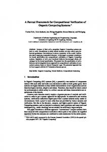
where, in (v) = w1 w2 . . . wn and Si = (fwi , awi ,v , Pwi ) with i > 1, is a tuple which gives, for spare l(wi ) the failure signal (fwi ), the activation signal by SPARE gate l(v) (awi ,v ) and the set of activation signals emitted by all SPARE gates (except v ) sharing spare l(wi ): Pwi = {awi ,g | (wi , g) ∈ E ∧ g = v ∧ type(g) = SPARE }. To compute the reliability of D, we are only interested in the failure of the top node T . Hence, we hide all signals except fT , i.e. we compute MD = hide AD \ fT in D; recall that AD denotes the set of all actions in D. The compositional aggregation technique described in Section VII is an efficient way to derive MD . Example 2 Figure 12 shows the I/O-IMC semantics of a DFT consisting of a SPARE gate A having a primary B and a spare C . Since the DFT contains no FDEP gates, we ignore all firing auxiliaries. The I/O-IMC of the DFT is obtained by parallel composing A, B, and C. A = (SPARE , 2)ELT (fA , aA , fB , (fC , aC,A , ∅)) AA(aA , ∅) B = (BE , 0, λ, 0)ELT (aB , fB ) AA(aB , ∅) C = (BE , 0, λ, μ)ELT (aC , fC ) AA(aC , {aC,A })

fB ?

A

fC ?

B

C

AA(aB , ∅) aB !

aA ? fB !

λ

fC ? aC,A !

CELT μ λ

fC ?

fC ! fC ?

Fig. 12.

aA !

aA ?

aA ?

fB ?

aC ?

AA(aA , ∅)

fC ? fB ?

BELT aB ?

AELT

fB ?

fA !

AA(aC , {aC,A }) aC,A ?

aC !

A DFT example and the six I/O-IMCs that model its behavior.

VI. DFT

ELEMENTS EXTENSION

In this section, we show, through three examples, how one can readily extend the DFT elements within the I/O-IMC framework. These extensions concern the modeling of inhibition, mutually exclusive events, and repair. Adding/modifying elements is done at the level of the elementary I/O-IMC models. Moreover, adding/modifying one element

This article has been accepted for publication in a future issue of this journal, but has not been fully edited. Content may change prior to final publication. IEEE TRANSACTIONS ON DEPEDABLE AND SECURE COMPUTING 11 r!

does not affect the remainder of the elements (i.e. their corresponding I/O-IMC models). This is indeed a desirable property of the I/O-IMC framework, where the behavioral details and interactions of any element is kept as local as possible. These extensions only affect Step 1 of the DFT conversion/analysis algorithm laid out in Section VII, leaving the other five steps unchanged. Inhibition and mutual exclusion. We say that event A inhibits the failure of B if the failure of B is prevented when A fails before B . Following the idea of the firing auxiliary (cf. Section V), this could be modeled by simply adding an inhibition auxiliary (IA). Figure 13 shows the configuration of such inhibition and the ∗ corresponding I/O-IMC model of the IA of B . fB corresponds to the failure signal of B taken in isolation, i.e. without A’s inhibition. Note that, as with the FA, any element which has B as input has to now interface with B ’s IA rather than directly with B. If A inhibits the failure of B and B also inhibits the failure of A, the failure of A and the failure of B become two mutually exclusive events. Clearly, this can be modeled in our framework by adding IAs for both A and B . Mutual exclusion is very useful for modeling different failures of a single component with different effects (e.g. a valve being stuck open or closed). fB fA

IAB

A

Fig. 13.

fB !

∗ fB ?

∗ fB

fA ? B

The I/O-IMC model of the IA.

Repair. Adding a notion of repair is somewhat more complicated as every DFT element can now fail or be repaired. Thus, no longer only a ‘failed event’ should be signaled but also a ‘repaired event’. However, as mentioned above, we only need to modify ‘locally’ the elementary I/O-IMC corresponding to each DFT element behavior. Here we will only discuss the new I/O-IMC for the BE and the AND gate (other elements are treated in the same fashion). The repairable cold BE’s I/O-IMC is shown in Figure 14. Here, μ denotes the BE repair rate and r! is a signal output by the BE notifying the rest of the elements that it has been repaired. The repairable AND gate I/O-IMC model is shown a?

Fig. 14.

λ

f!

r!

μ

The repairable BE I/O-IMC model.

in Figure 15. The AND gate has its own repair output signal (i.e. r!) and needs to consider both failure (fA ? and fB ?) and repair (rA ? and rB ?) signals coming from its inputs A and B . Compared to the unrepairable AND gate (Figure 9), Figure 15 has 3 extra states. If we consider a very simple repairable system composed of an AND gate with two BE A and B (Figure 16 (left)), then the resulting I/O-IMC after automatic composition, hiding of all signals and aggregation is, as expected, the CTMC shown in Figure 16 (right). At this point, one can perform analysis on the CTMC such as computing the system unavailability.

r!

rB ?

fB ?

fA ? rA ?

rB ?

fB ?

fA ?

rB ?

fA ? f!

rA ? fB ? rB ?

rA ?

fB ?

rA ? fA ?

r!

Fig. 15.

The repairable AND gate I/O-IMC model. λA

A

B

λB

μA

μB

λB

λA

μB

μA

Fig. 16. A simple repairable system. The gray state denotes the state in which the DFT has failed.

VII. C OMPOSITIONAL AGGREGATION APPROACH The technique of compositional aggregation consists of composing a large model out of smaller ones and aggregating submodels after each compositional step. This approach is to be contrasted with a more classical approach of model generation, such as the one used by Galileo DIFTree [21], where the model of a system is generated at once and as a whole and then eventually aggregated at the end. Compositional aggregation is very effective in combating the state-space explosion problem and has been already successfully used on a number of case studies, most notably in [18]. Once the DFT elements have been converted into a set of I/OIMCs, the compositional aggregation methodology can be applied to combine the set into a single I/O-IMC. The final I/O-IMC reduces in many cases to a CTMC. This CTMC can then be solved using standard methods [24] to compute performance measures such as system unreliability. The conversion/analysis algorithm9 is as follows: 1) Map each DFT element to its corresponding (aggregated) I/O-IMC and match all inputs and outputs. The result of this step is a set of I/O-IMCs. 2) Pick two I/O-IMC and parallel compose them. 3) Hide output signals that won’t be subsequently used (i.e. synchronized on). 4) Aggregate (using weak bisimulation) the I/O-IMC obtained from the composition of the two I/O-IMC picked in Step 2 and the hiding of the output signals in Step 3. 5) Go to Step 2 if more than one I/O-IMC is left, otherwise go to Step 6. 6) Analyse the aggregated CTMC. The choice of I/O-IMCs made in step 2 is important as it influences the size of the generated state-space during the intermediate steps. If no non-determinism is present in the DFT model, then the algorithm yields a CTMC. However, in some cases where non-determinism arises, the result is a continuous-time Markov decision process, which can be analyzed by computing bounds on the performance measure of interest [2]. 9 Note

that this algorithm is amenable to parallelization.


VIII. T OOL SUPPORT In this section we describe the CORAL [6] tool chain which supports our DFT analysis methodology. The tools presented in this section use the CADP tool-set [15] for many operations on I/O-IMCs, such as composition, aggregation and CTMC analysis. Before discussing the various tools in detail we will first give an overview of the tool chain. Tool chain overview. Figure 17 shows an overview of the tool chain for our DFT analysis methodology. The user must supply DFT (ext. Galileo format)

Composition script

CORAL I/O-IMC models

dft2bcg

SVL

bcg labels

SVL

DFT elements I/O-IMCs repository

I/O-IMC model

composer

acyc min

dft eval CTMC model + goal state

Mission times

Key:

Fig. 17.

Uses

Unreliability

bcg transient

CORAL component

CADP component

Data

An overview of the CORAL tool chain.

the following input: the DFT in a file using the Galileo format, a composition-script denoting the order of composition used in the compositional aggregation phase and the mission times for the unreliability analysis. . A DFT can be analyzed by performing the following three steps, which are elaborated below. 1) Call the dft2bcg tool with as input the DFT file in extended Galileo format10 , 2) Call the composer tool with as input a composition script, and 3) Call the dft eval tool with as input a number of missiontimes. The dft eval tool then calculates the unreliability of the system modeled by the original DFT for the given mission-times. It generates a CTMC model describing the exact failure distribution of the system if there is no nondeterminism. Generating I/O-IMC models: dft2bcg. The dft2bcg tool generates a number of I/O-IMC models that describe the behaviour of a given DFT. To be more exact, each of the I/O-IMCs describes one element in the DFT (see Section V). These I/O-IMC models are 10 The standard Galileo format is extended to allow complex spares and dependent events

stored in binary coded graph (BCG) format supported by CADP. The dft2bcg tool uses a number of script verification language (SVL) scripts to generate BCG files. These scripts are interpreted by the SVL tool, which is part of the CADP tool set, to perform generation, parallel composition, hiding and minimization of BCG files. dft2bcg also uses the bcg labels tool of the CADP tool-set which allows the renaming of the actions of an I/O-IMC. The dft2bcg tool performs the following steps to generate the I/O-IMC models: 1) Parses the DFT input file, 2) Checks the validity of the DFT (i.e. syntactic check), 3) Calls the SVL tool to generate I/O-IMC models with generic action names (f1 , f2 , . . .) using the DFT SVL scripts, and 4) Calls the bcg labels tool to create the I/O-IMC models by renaming the generic actions to the specific actions derived from the names of the DFT elements. All generic models generated in step 3 are stored in a DFT repository for reuse in later calls of the dft2bcg tool. For instance if we need three different 3-input AND-gates we can simply use the same generic 3-input AND gate, renaming it differently in step 4 of the dft2bcg tool. The repository also holds a number of basic I/O-IMC models which are used to generate the models of all DFT elements. Compositional aggregation: composer. We have seen above that the dft2bcg tool generates a number of I/O-IMC models. The composer tool uses as input these I/O-IMC models and a composition script supplied by the user. The composition script describes the order in which the I/O-IMC models should be composed. The composer tool executes the commands in the script, composing the I/O-IMC models into a single I/OIMC model which represents the stochastic behaviour of the entire DFT. Our choice of composition script is based on heuristics, such as maximizing the number of transitions that will be hidden and minimizing the number of actions that are not synchronized. After each composition the resulting I/O-IMC model is minimized using the acyc min tool [12]. The acyc min tool minimizes acyclic (except for self-loops with input-actions) I/O-IMCs with respect to weak bisimulation for I/O-IMCs (see Section III). Calculating measures: dft eval. In many cases the stochastic behaviour of the system described by a DFT can be modelled as a CTMC. To be more specific: if there is no non-determinism present in the DFT model of the system the I/O-IMC generated in our approach reduces to a CTMC. See Section II-A for a detailed discussion on the occurrence of non-determinism in DFT analysis. The dft eval tool first reduces the I/O-IMC representation of the DFT into a CTMC and then invokes the CADP tool bcg transient to find the unreliability of the DFT for a set of mission-times supplied by the user. IX. C ASE STUDIES We have assessed the efficiency of our compositional aggregation approach by performing nine case studies from different application areas. We analyzed a cascaded PAND system (CPS), two versions of a cardiac assist system (CAS), five versions of a fault tolerant parallel processors (FTPP), and finally a pump system with inherent non-determinism. We systematically compare our results (using the CORAL tool) to the Galileo DIFTree tool [14] results, see Table I for an overview. Here, the number


of states/transitions corresponds to the largest I/O-IMC or CTMC encountered during analysis. All experiments were run on an AMD Athlon XP 2600+ running at 1.9 GHz with 1 GB memory. The cascaded PAND system. This system, taken from [7] and shown on Figure 18 (left), illustrates the enhanced modularity of our methodology compared to Galileo DIFTree. In fact, given that the top node of the tree is a PAND dynamic gate, Galileo DIFTree can only consider the tree as a whole when generating/solving its corresponding CTMC. In our compositional aggregation approach, we realize that there are independent modules, in particular A, C, and D are all identical (all BEs have a failure rate equals to 1) and independent modules. In fact it suffices to generate and aggregate the I/O-IMC of one of these three modules and reuse the result, given some renaming of signals, for the remaining two modules. In this way, A, C, and D have each an aggregated I/OIMC of 7 states only. The CTMC generated by Galileo has 4113 states. This result is to be compared with the largest I/O-IMC of 113 states obtained during the compositional aggregation.

Pumps

Motors A

CPUs

B

C

P

D

Fig. 18.

MS

MA MB PA

PS

PB

DFTs for CPS (left) and CAS (right) case studies

2/3

A1

Component Rate

B

CS SS

2/3

A2

A3

B1

B2

AS N1

2/3

B3

C1

BS N2

C2

2/3

C3

D1

CS

D2

D3

DS

N3

N4

A1 B1 C1 D1 A2 B2 C2 D2 A3 B3 C3 D3 A4 B4 C4 D4

Fig. 19.

DFT for the FTPP-4 case study

Case study CPS CAS CAS-PH FTPP-4 FTPP-5 FTPP-6 FTPP-C FTPP-A NDPS

Approach Galileo CORAL Galileo CORAL CORAL Galileo CORAL CORAL CORAL CORAL Galileo CORAL CORAL

Max # of states 4113 133 8 36 40052 32757 1325 43105 1180565 653303 32757 19367 61

with a dormancy factor α = 0.5, and MB and PS are cold spares (i.e. α = 0). During analysis, Galileo DIFTree modularizes the DFT into three independent modules (namely CPU, motors, and pump units) and generates a separate CTMC for each one of them. The biggest CTMC has 8 states. The CTMCs’ results are then combined (through the top OR gate) using BDDs. Using the compositional-aggregation approach, and without modularization, the biggest I/O-IMC encountered has 36 state. The results of CAS are summarized in Table I. Here, clearly Galileo outperforms CORAL because it uses modularization which has not been implemented yet in CORAL. If we switch off modularization in Galileo (i.e. generate a single CTMC for the whole system) then it produces a CTMC with 85 states. To illustrate the possibility of using phase-type distributions we have modified the CAS case study by replacing BEs with PHBEs (case CAS-PH). In this case all basic events occur after a delay governed by an Erlang distribution with four phases and the same expectation as the exponential delay from the CAS case study (for instance, PHBE CS is governed by a 4-phase Erlang with rate parameter 0.8 instead of an exponential distribution with rate 0.2). For the passive delay of warm spare B we also use an Erlang distribution with four phases and the same expectation as the passive exponential delay.

Max # of transitions 24608 465 10 119 265442 426826 13642 643339 22147378 12220653 426826 154566 169

Unreliability (time = 1) 0.00135 0.00135 0.65790 0.65790 0.112826 0.01922 0.01922 0.00306 0.000453 0.02136 0.0167 0.0167 [0.00586, 0.00598]

Time (sec) 490 67 1 94 231 13111 65 309 1989 1806 13111 240 266

TABLE I R ESULTS OF THE CASE STUDIES .

The cardiac assist system. This system, taken from [5] and shown in Figure 18 (right), consists of a three separate modules (i.e. CPU, motors, and pump units). Table II shows the failure rates of the various components. In addition, B is a warm spare

CS 0.2

SS 0.2

P 0.5

B 0.5

MA 1

MB 1

MS 0.01

PA 1

PB 1

PS 1

TABLE II FAILURE RATES FOR CAS.

The fault tolerant parallel processors. This system, taken from [5], consists of 16 processors divided into 4 logical groups. In each group, a processor is used as a shared cold spare. A network element (NE) physically connects 1 processor in each group (thus there are 4 NEs) to the rest of the system. The failure of an NE makes the 4 processors connected to it unavailable (i.e. essentially failed). The requirement is to have at least two processors operational in each group. The DFT is shown in Figure 19, where the processors are denoted with Ai ,Bi ,Ci ,Di and the network elements with N. All network elements have a failure rate equals to 0.017, and all processors have a failure rate equals 0.11. The four spare processors are cold spares (i.e. α = 0). To illustrate even further the state-space explosion problem, we took the FTPP system and made it larger by considering 5 (FTPP5) respectively 6 (FTPP-6) processors in each group. For these case studies the Galileo tool runs out of memory. The (FTPP-C) case study is an extension to the FTPP system where each of the processors (e.g. A1 ) is replaced by a complex element which consists of an OR-gate with two inputs: a BE ‘CPU’ and a spare gate ‘memory’ with primary BE ‘M1’ and cold spare BE ‘M2’. All these BEs have failure rate 0.11. No results are available from Galileo DIFTree as this kind of extended DFTs can not be handled by Galileo. It is interesting to investigate how dependent the success of the compositional aggregation technique is on the symmetries in the DFT models. In the case study FTPP-A we have therefore considered a variant of the FTPP case study where almost all basic events have different rates. The rates used are given in Table III. We see that indeed the models encountered are larger by a factor of 15, but still the computational time required is manageable at under 5 minutes. Non-deterministic pump system (NDPS). This case study il-


BE N1 N2 N3 N4

Rate 3.4 2.9 2.4 1.7

BE A1 A2 A3 A4

Rate 5.5 7.7 14 18

BE B1 B2 B3 B4

Rate 11 15.4 28 36

BE C1 C2 C3 C4

Rate 6.6 99 16 22

BE D1 D2 D3 D4

Rate 7.7 11 22 30

TABLE III FAILURE RATES FOR FTPP-A. R ATES ARE SCALED UP BY A FACTOR 105 .

lustrates how we deal with non-determinism in DFT models. The I/O-IMC model of the DFT is generated as usual and then converted into a CTMDP following [17]. This CTMDP is then analyzed using the MRMC [19] tool to obtain maximum and minimum unreliability. The DFT is a simple pumping system with five pumps: main pumps A and B , auxiliary pumps C , D and spare auxiliary pump E (see Figure 20). BE A has rate 0.05 and BE B has rate 0.1; BEs C and D both have rate 0.2 and BE E has rate 0.3 with dormancy α = 0. Finally BE X has rate 0.002. This DFT is non-deterministic since C and D may fail at the same time due to their dependence on BE X . It is then undetermined whether spare E replaces C or D. We can see that the maximum and minimum unreliabilities are not far apart, this is caused by the low probability of the ‘problematic’ BE X .

X A

B C

Fig. 20.

D

E

DFT for NDPS case study X. C ONCLUSION AND FUTURE WORK

In this paper we have formalized the syntax and semantics of DFTs and introduced a DFT analysis framework based on I/O-IMCs, increasing the DFT modularity both at the analysis level and the model-building level. We have also demonstrated the ease with which one can define new DFT elements and provided examples of such extensions. Finally, we have built a prototype tool for analysing DFTs named CORAL and run some experiments to compare our methodology and results to the Galileo DFT tool. Areas of future research include: (1) From a process algebra point of view, we would like to achieve even more drastic statespace reduction using more suitable aggregation techniques. (2) Adapt the I/O-IMC approach to other formalisms, such as the Architecture Analysis and Design Language [1]. A first step towards this goal has been made in [4]. Acknowledgements: We thank Holger Hermanns and the anonymous reviewers of this paper for their helpful comments. R EFERENCES [1] As-2 Embedded Computing Systems Committee. Architecture analysis & design language (AADL), January 2009. Number: AS5506, Revision: A. [2] C. Baier, H. Hermanns, J. P. Katoen, and B. R. Haverkort. Efficient computation of time-bounded reachability probabilities in uniform continuous-time markov decision processes. Theor. Comput. Sci., 345(1):2–26, 2005.

[3] E. Böde, M. Herbstritt, H. Hermanns, S. Johr, T. Peikenkamp, R. Pulungan, J. Rakow, R. Wimmer, and B. Becker. Compositional dependability evaluation for statemate. IEEE Trans. Software Eng., 35(2):274–292, 2009. [4] H. Boudali, P. Crouzen, B. R. Haverkort, M. Kuntz, and M. Stoelinga. Architectural dependability evaluation with arcade. In Proceedings of the 38th IEEE/IFIP International Conference on Dependable Systems and Networks, pages 512–521, 2008. [5] H. Boudali, P. Crouzen, and M. Stoelinga. A compositional semantics for Dynamic Fault Trees in terms of Interactive Markov Chains. In Proceedings of the 5th International Symposium on Automated Technology for Verification and Analysis, pages 441–456. LNCS, 2007. [6] H. Boudali, P. Crouzen, and M. Stoelinga. Coral – a tool for compositional reliability and availability analysis. In ARTIST WS: Tool Platforms for ES Modelling, Analysis and Validation, 2007. [7] H. Boudali, P. Crouzen, and M. Stoelinga. Dynamic fault tree analysis using input/output interactive markov chains. In Proceedings of the 37th IEEE/IFIP International Conference on Dependable Systems and Networks, pages 708–717, June 2007. [8] M. A. Boyd. Dynamic fault tree models: techniques for analyses of advanced fault tolerant computer systems. PhD dissertation, Dept. of Computer Science, Duke University, 1991. [9] M. Bravetti and R. Gorrieri. The theory of interactive generalized semimarkov processes. Theoretical Computer Science, 282(1):5–32, 2002. [10] D. Coppit, K. J. Sullivan, and J. B. Dugan. Formal semantics of models for computational engineering: A case study on dynamic fault trees. In Proceedings of the International Symposium on Software Reliability Engineering, pages 270–282. IEEE, Oct 2000. [11] N. Coste, H. Garavel, H. Hermanns, R. Hersemeule, Y. Thonnart, and M. Zidouni. Quantitative evaluation in embedded system design: Validation of multiprocessor multithreaded architectures. In Design, Automation and Test in Europe, pages 88–89, 2008. [12] P. Crouzen, H. Hermanns, and L. Zhang. On the minimisation of acyclic models. In Proceedings of the 19th International Conference on Concurrency Theory, pages 295–309, 2008. [13] J. B. Dugan, S. J. Bavuso, and M. A. Boyd. Dynamic fault-tree models for fault-tolerant computer systems. IEEE Transactions on Reliability, 41(3):363–377, September 1992. [14] J. B. Dugan, B. Venkataraman, and R. Gulati. DIFTree: a software package for the analysis of dynamic fault tree models. In Reliability and Maintainability Symposium, pages 64–70, Jan 1997. [15] H. Garavel, F. Lang, R. Mateescu, and W. Serwe. Cadp 2006: A toolbox for the construction and analysis of distributed processes. In Proceedings of the 19th International Conference on Computer Aided Verification (CAV), 2006. [16] H. Hermanns. Interactive Markov Chains, volume 2428/2002 of Lecture Notes in Computer Science. Heidelberg: Springer Berlin, 2002. [17] H. Hermanns and S. Johr. Uniformity by construction in the analysis of nondeterministic stochastic systems. In Proceedings of the 37th IEEE/IFIP International Conference on Dependable Systems and Networks, pages 718–728, 2007. [18] H. Hermanns and J. P. Katoen. Automated compositional Markov chain generation for a plain-old telephone system. Science of Computer Programming, 36(1):97–127, 2000. [19] J.-P. Katoen, M. Khattri, and I. S. Zapreev. A markov reward model checker. In Proceedings of the 2nd Second International Conference on the Quantitative Evaluation of Systems, pages 243–244, 2005. [20] N. A. Lynch and M. R. Tuttle. An introduction to input/output automata. CWI Quarterly, 2(3):219–246, 1988. [21] R. Manian, J. B. Dugan, D. Coppit, and K. J. Sullivan. Combining various solution techniques for dynamic fault tree analysis of computer systems. IEEE International High-Assurance Systems Engineering Symposium, 3:21–28, 1998. [22] M. F. Neuts. Matrix-Geometric Solutions in Stochastic Models: An Algorithmic Approach. Dover, 1981. [23] Relex, Fault Tree and Event Tree software. http://www.relex.com/products/ftaeta.asp. Relex Website. [24] W. J. Stewart. Introduction to the Numerical Solution of Markov Chains. Princeton University Press, 1994. [25] K. J. Sullivan, J. B. Dugan, and D. Coppit. The Galileo fault tree analysis tool. In Proceedings of the 29th Annual International Symposium on Fault-Tolerant Computing, pages 232–235. IEEE Computer Society, June 1999. [26] K. K. Vemuri, J. B. Dugan, and K. J. Sullivan. Automatic synthesis of fault trees for computer-based systems. IEEE Transactions on Reliability, 48(4):394–402, December 1999.


A PPENDIX I P ROOFS

[27] W. E. Veseley, F. F. Goldberg, N. H. Roberts, and D. F. Haasl. Fault tree handbook, NUREG-0492. Technical report, NASA, 1981.

A. Theorem 1.1 Hichem Boudali received a Ph.D. degree in Computer Engineering from the School of Engineering and Applied Science at the University of Virginia (Charlottesville, VA, USA), in 2005. He received a Computer Science Engineering degree (M.Sc. equivalent) from the Polytechnic School and Applied Sciences at the Universit Libre de Bruxelles (Brussels, Belgium), in 2002. The same year, he obtained a M.Sc. degree in Electrical Engineering from the University of Virginia. He is also a member of IEEE.

Pepijn Crouzen received a Computer Science Engineering degree (M.Sc. equivalent) from the University of Twente (Enschede, The Netherlands) in 2006. He is now a PhD student in the Dependable Systems and Software group of the Computer Science faculty of Saarland University (Saarbrücken, Germany).

For weak bisimilarity on an I/O-IMC P , ≈P , we find: 1) ≈P is a weak bisimulation on P and it is the largest weak bisimulation on P . Proof: We now prove that for any I/O-IMC P ≈P is the largest weak bisimulation on P . In the following we refer to ≈P simply as ≈. To do this we must prove that ≈ is an equivalence relation by proving that it is reflexive, symmetric and transitive. The proofs for reflexivity and symmetry are quite simple, but the proof for transitivity is somewhat more complex. For any I/O-IMC P it is trivial that the identity relation IdP is a weak bisimulation. For any state s in SP we find that (s, s) ∈ IdP and thus s ≈ s. In other words ≈ is reflexive. If s ≈ t then there is a weak bisimulation R with (s, t) ∈ R. Because R is an equivalence relation we also find that (t, s) ∈ R and so t ≈ s. We now find that s ≈ t implies t ≈ s. This means that ≈ is symmetric. Let R1 and R2 be two weak bisimulations on P and let R1 R2 ∗ be defined as their recursive composition: R1 R2 ∗ = {(s, t) | ∃n ∈ N, x1 , ..., xn ∈ S· (s, x1 ) ∈ R1 ∪ R2 ∧ ... ∧ (xn , t) ∈ R1 ∪ R2 }

Mariëlle Stoelinga received her Ph.D. in Computer Science from the University of Nijmegen, the Netherlands, in 2002. She is currently an assistant professor at the Formal Methods & Tools group at the University of Twente, the Netherlands.

Because R1 and R2 are equivalence relations it is trivial that R1 R2 ∗ is reflexive and symmetric. From the definition of R1 R2 ∗ we can also immediately deduce that it is a transitive relation. We will now prove that R1 R2 ∗ is a weak bisimulation relation. Recall that if (s, t) is in R1 R2 ∗ then there exist a series of states x1 , ..., xn such that they are stepwise related through either R1 or R2 : sRi x1 Ri x2 ...xn Ri t where Ri is R1 or R2 . We find that a a for any action a ∈ Aall P with s=⇒s there is an x1 with x1 =⇒x1 and (s , x1 ) ∈ R1 ∪ R2 . This in turn means that there is an x2 a with x2 =⇒x2 and (s , x2 ) ∈ R1 ∪ R2 . So we find a series of states x1 , ..., xn , t such that (s , x1 ) ∈ R1 ∪ R2 ∧ ... ∧ (xn , t ) ∈ a R1 ∪ R2 . Thus t=⇒t with (s , t ) ∈ R1 R2 ∗ , which means that the first clause of Definition 4 holds. To prove that the second clause holds we must first consider the equivalence classes of R1 R2 ∗ . From the definition we know that R1 ⊆ R1 R2 ∗ and R2 ⊆ R1 R2 ∗ . This means that any equivalence class of R1 R2 ∗ is exactly the union of one or more equivalence classes of R1 and it is also exactly the union of one or more equivalence classes of R2 . So for any equivalence class C of R1 R2 ∗ we find that there is a set C1 , C2 , ...Cn of equivalence classes of R1 and a set C1 , C2 , ...Cm of equivalence classes of R2 with n, m > 0 such that: C = C1 ∪ C2 ∪ ... ∪ Cn = C1 ∪ C2 ∪ ... ∪ Cm

It is trivial that this also holds for the internal backwards closure of an equivalence class of R1 R2 ∗ : int C int = C1int ∪ C2int ∪ ... ∪ Cnint = C1int ∪ C2int ∪ ... ∪ Cm

For a state s we find that it’s equivalence class for R1 R2 ∗ : [s]R1 R2 ∗ contains all states t such that (s, t) ∈ R1 R2 ∗ . Because (s, t) ∈ R1 implies (s, t) ∈ R1 R2 ∗ we find that [s]R1 ⊆ [s]R1 R2 ∗ and similarly [s]R2 ⊆ [s]R1 R2 ∗ . Because equivalence classes are disjoint we now find that if an equivalence class of R1 R2 ∗ : C = [s]R1 R2 ∗ then C ∩ [s]R1 = ∅ and also C ∩ [s]R2 = ∅.


Let (s, t) ∈ R1 R2 ∗ and let there be a s such that s=⇒s and s is stable. If (s, t) ∈ R1 ∪ R2 then the second clause of Definition 4 holds. Otherwise there exists an x1 such that (s, x1 ) ∈ R1 ∪ R2 , so either (s, x1 ) ∈ R1 or (s, x1 ) ∈ R2 . For the first case we find that there is an x1 such that x1 =⇒x1 and x1 stable and γM (s , C int ) = γM (x1 , C int ), for all equivalence classes C of R1 except [s ]R1 . For the second case we find that there is an x1 such that: x1 =⇒x1 and x1 stable and γM (s , C int ) = γM (x1 , C int ), for all equivalence classes C of R2 except [s ]R2 . So we find that there is always an x1 such that x1 =⇒x1 and x1 stable and γM (s , C int ) = γM (x1 , C int ), for all equivalence classes C of R1 R2 ∗ except [s ]R1 R2 ∗ . Note that the equivalence classes [s ]R1 and [s ]R2 must be contained in [s ]R1 R2 ∗ and not in any other equivalence class of R1 R2 ∗ . The same holds for the pairs (x1 , x2 ), (x2 , x3 ), ..., (xn , t), so in the end we find that the second clause of Definition 4 holds for R1 R2 ∗ so R1 R2 ∗ is a weak bisimulation. If we now have that s ≈P x and x ≈P t then there exist two weak bisimulations R1 and R2 such that (s, x) ∈ R1 and (x, t) ∈ R2 . Then (s, t) ∈ R1 R2 ∗ and because R1 R2 ∗ is a weak bisimulation on P we find that s ≈P t which means that ≈P is an equivalence relation. Because ≈P is the union of all weak bisimulations on P it is trivial that ≈P itself is a weak bisimulation now that we have proved that it is an equivalence relation. That ≈ is the largest weak bisimulation on P follows immediately from its definition. B. Theorem 1.2 and 1.3

From the definition of R we can deduce that it has the following equivalence classes: S/R = {{x y | x ∈ C} | C ∈ SP /R, y ∈ SP3 }

Because (s, s ) ∈ R if and only if ∀u ∈ SP3 · (s u, s u) ∈ R we find that for an equivalence class [s u]R : [s u]R = {s u | s ∈ [s]R }. Now let (s u, t u) ∈ R with s u=⇒s u and s u stable and let C be an equivalence class of R with C = [s u ]R . From the definition of parallel composition we know that this means that s=⇒s and u=⇒u and both s and u stable. We know that each equivalence class of R is derived from an equivalence class of R and a state in SP3 . Let D be that equivalence class of R and let y be that state. So C = {s y | s ∈ D} and u = y implies D = [s ]R . Note that if u = y , s u cannot be in C . Now we find the following for the internal backward closure of C : C int

implies

P1 ||P3 ≈ P2 ||P3

P1 ≈ P2

implies

P3 ||P1 ≈ P3 ||P2

Proof: We now prove that weak bisimilarity is substitutive with parallel composition. Let P1 and P2 be I/O-IMCs with identical action signatures, let P be their union and let x ≈P y . This means that there is a weak bisimulation R on P such that (x, y) ∈ R. We now define the relation R as follows: R = {(x z, y z) | (x, y) ∈ R ∧ z ∈ SP3 }

Because R is an equivalence relation on P it is trivial that R is also an equivalence relation on P ||P3 . a Let (s u, t u) ∈ R , then (s, t) is in R. Now let s u=⇒s u all with a ∈ A . This means that there exist s u and s u such a that s=⇒s , u=⇒u , s u − →s u , s =⇒s and u =⇒u . From the definition of parallel composition we can deduce a that s u − →s u implies that one of the following holds: a a s − →s ∧ u = u ∧ a ∈ A(P ) ∧ a ∈ / A(P3 ) or u − →u ∧ s = a / A(P ) or s − →s ∧ u − →u ∧ a ∈ s ∧ a ∈ A(P3 ) ∧ a ∈ a A(P ) ∧ a ∈ A(P3 ). In other words either s=⇒s ∧ u=⇒u ∧ a ∈ a / A(P ) A(P ) ∧ a ∈ / A(P3 ) or u=⇒u ∧ s=⇒s ∧ a ∈ A(P3 ) ∧ a ∈ a or s=⇒s ∧ u=⇒u ∧ a ∈ A(P ) ∧ a ∈ A(P3 ). Because (s, t) ∈ R we find that there is a t with (s , t ) ∈ R such a a that: t=⇒t ∧ u=⇒u ∧ a ∈ A(P ) ∧ a ∈ / A(P3 ) or u=⇒u ∧ a / A(P ) or t=⇒t ∧ u=⇒u ∧ a ∈ t=⇒t ∧ a ∈ A(P3 ) ∧ a ∈ A(P ) ∧ a ∈ A(P3 ). From the definition of parallel composition a we now know that: t u=⇒t u and from the definition of R we know that (s u , t u ) is in R . This means that the first clause of Definition 4 holds for R .

{x y | ∃x y ∈ C · x y =⇒x y}

=

{x y | ∃x ∈ D · x =⇒x ∧ y =⇒y}

If we now look at the cumulative rate of s u to C int we find: γM (s u , C int ) X λ →M x = {|λ | ∃x ∈ D · s − X λ →M y {|λ | ∃x ∈ D · u − X λ →M x = {|λ | ∃x ∈ D · s − X λ →M y {|λ | ∃x ∈ D · u −

∧ x =⇒x ∧ u =⇒y|} + ∧ s =⇒x ∧ y =⇒y|} ∧ x =⇒x ∧ u = y|} + ∧ s = x ∧ y =⇒y|}

(Because s and u are stable)

Weak bisimilarity is substitutive with parallel composition. P1 ≈ P2

=

=

=

8 int int > > >γM (s , D ) + γM (u , {y} ) , if u > , if u >γM (u , {y} ) > > : 0 , if u 8 int , if u = y ∧ s ∈ /D > : 0 , if u = y ∧ s ∈ /D

= y ∧ s ∈ D = y ∧ s ∈ /D = y ∧ s ∈ D = y ∧ s ∈ /D

(Because u = y implies D = [s ]R .) Because (s, t) ∈ R we know that s=⇒s and s stable imply that there is a t such that t=⇒t and t stable with (s , t ) ∈ R11 and γM (s , Dint ) = γM (t , Dint ) for every equivalence class D of R except [s ]R . It is furthermore trivial that s and t are in the same equivalence class of R. We now conclude that: γM (s u , C int ) 8 int > : 0 8 int > : 0

, if u = y ∧ s ∈ /D , if u = y ∧ s ∈ D , if u = y ∧ s ∈ /D , if u = y ∧ t ∈ /D , if u = y ∧ t ∈ D , if u = y ∧ t ∈ /D

(Because s ∈ / D implies that D = [s ]R .) =

γM (t u , C int )

11 Because (s, t) ∈ R and s=⇒s there is a y such that t=⇒y and (s , y) ∈ R. For this pair clause 1 and 2 of weak bisimulation must hold once more. Eventually we will find t this way.


So clause two of Definition 4 holds for R . For any state z ∈ SP3 we find that if (x, y) ∈ R then (x z, y z) ∈ R and since R is a weak bisimulation x z ≈ y z thus proving Theorem 1.2. We find a similar proof for Theorem 1.3 because parallel composition is completely symmetric. This then proves that weak bisimilarity is substitutive with parallel composition.

of hide B in s to C int : γM (hide B in s , C int ) =

{|λ | ∃(hide B in x ) ∈ S, (hide B in x) ∈ C · λ

→M hide B in x ∧ hide B in s − hide B in x =⇒hide B in x|} =

{|λ | ∃(hide B in x ) ∈ S, x ∈ D · λ

→M hide B in x ∧ hide B in s − hide B in x =⇒hide B in x|}

C. Theorem 1.4 Weak bisimilarity is substitutive with hiding. P1 ≈ P2 implies hide a1 , ..., an in P1 ≈ hide a1 , ..., an in P2

Proof: Let P1 and P2 be I/O-IMCs with identical action signatures, let P be their union. Then if P1 ≈ P2 there is a weak bisimulation R on P such that ∀s ∈ SP1 · ∃t ∈ SP2 · (s, t) ∈ R. Let B ⊆ AV (P ) = {a1 , . . . , an } be a subset of the visual actions of P and let R be a binary relation defined as follows: R = {(hide B in s, hide B in t) | (s, t) ∈ R}

It is trivial that R is an equivalence relation on hide B in P . a Let hide B in s=⇒hide B in s . From the definition of hiding we can immediately deduce that there exists an n ∈ N with n ≥ 0, a series of states x1 , ..., xn and a series of actions b1 , ..., bn ∈ B such that: b

b

a

bn−1

b

1 2 n s=⇒x 1 =⇒...xk =⇒xk+1 ... =⇒ xn =⇒s

Because (s, t) ∈ R we find a series of states x1 , ..., xn−1 such that: b

b

a

bn−1

b

1 2 n t=⇒x 1 =⇒...xk =⇒xk+1 ... =⇒ xn =⇒t

a

It follows that hide B in t=⇒hide B in t so the first clause of Definition 4 holds for R . Let hide B in s=⇒hide B in s and hide B in s stable. This means that there is an n ∈ N, a series of actions b1 , ..., bn b1 and a series of states x1 , ..., xn such that s=⇒x 1 ...xn =⇒s with b1 , ..., bn ∈ B . For t we then find the same series of actions and a weakly bisimilar set of states. We particularly find an xn such that (xn , xn ) ∈ R. Because xn =⇒s and s stable we find a t such that xn =⇒t and t stable with γM (s , D) = γM (t , D) for all equivalence classes D of R except for [s ]R and (s , t ) ∈ R. Because hide B in s is stable s and t have no outgoing transitions labelled with an action in B . From the definition of R we see that its equivalence classes can be defined as follows: {{hide B in x | x ∈ D} | D ∈ S/R}

Note that for any state x in S we find that [hide B in x]R = {hide B in y | y ∈ [x]R }. Let C be an equivalence class of R with C = [hide B in s ]R and let D be the corresponding equivalence class of R, thus D = [s ]R . We now find the following for the cumulative rate

=

λ

→M x ∧ {|λ | ∃x ∈ S, x ∈ D · s − hide B in x =⇒hide B in x|}

=

γM (s , Dint+ )

Here Dint+ = {x | ∃x ∈ D · hide B in x =⇒hide B in x}. Note that Dint+ ⊇ Dint . For some n ∈ N let E1 , ..., En be the equivalence classes of R that can reach D with a number of weak transitions labelled with actions in B or with a weak move (note that this means that D itself is always in E1 , ..., En ). In other words we find that: ∀Ex · (∀e ∈ Ex · ∃m ∈ N, f1 , ..., fm ∈ S, b1 , ..., bm ∈ B· b

b

1 m m ≥ 0 ∧ e=⇒f 1 ...fm−1 =⇒fm ∧ fm ∈ D)

When we hide the set of actions B in the states of the equivalence classes Ex we find that they move internally to states in equivalence class C . Note that because hide B in s is stable and C = [hide B in s ]R , [s ]R can not be in E (that would either mean that hide B in s moves internally to a state in C making it unstable or that hide B in s is in C but this is not S possible because C = [hide B in s ]R ). So Dint+ = Ei Eiint . Now we find that γM (s , Dint+ ) = γM (t , Dint+ ) (Recall that we found earlier that γM (s , D) = γM (t , D) for all equivalence classes D of R except [s ]R which is not in E ). In the same way we showed that γM (hide B in s , C) equals γM (s , Dint+ ), we can now show that γM (t , Dint+ ) equals γM (hide B in t , C int ). This proves that the second clause of Definition 4 holds for R . This means that hide B in s ≈ hide B in t when s ≈ t and thus weak bisimilarity is substitutive with hiding.

A Rigorous, Compositional, and Extensible Framework for Dynamic

A Rigorous, Compositional, and Extensible Framework for Dynamic

Suggest Documents

An Extensible Modeling Framework for Dynamic ... - CiteSeerX

A dynamic and extensible workflow-oriented software framework for

A dynamic and extensible software framework for Image-Guided ...

A Framework for Extensible Languages

A standardized, extensible framework for optimizing

Extensible Dynamic Analysis for JML: A Case

Scalable extensible middleware framework for

A Formal Framework for Compositional Verification ...

A Compositional Framework for Programming ...

Adaptor Grammars: A Framework for Specifying Compositional ...

A framework for practical and rigorous impact monitoring by - IUCN

A Flexible and Extensible Framework for Delivering Designer Images ...

A Generic and Extensible Framework for Monitoring Energy ...

MoDisco: A Generic And Extensible Framework For Model Driven ...

HyPER: A Flexible and Extensible Probabilistic Framework for Hybrid ...

Dynamic and Extensible Exception Handling for Workflows: A Service ...

A Logical and Ontological Framework for Compositional Concepts of ...

A Middleware Framework for Dynamic Reconfiguration and

An Extensible Framework for Context-aware Communication ...

An extensible framework for automatic knowledge

An Extensible Framework for Data Cleaning

A Rigorous Framework for Optimization of Expensive ... - CiteSeerX

A Framework for Statistically Rigorous Simulation-Based Network

COMPOSITIONAL FRAMEWORK FOR REAL-TIME ... - CiteSeerX