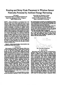
2009 IEEE 34th Conference on Local Computer Networks (LCN 2009) Zürich, Switzerland; 20-23 October 2009
A Robust Relay Node Placement Heuristic for Structurally Damaged Wireless Sensor Networks Fatih Senel and Mohamed Younis
Kemal Akkaya
Dept. of Computer Science & Elect. Engineering University of Maryland Baltimore County Baltimore, MD 21250 {fsenel1,younis}@cs.umbc.edu
Department of Computer Science Southern Illinois University Carbondale Carbondale, IL 62901
[email protected] strategy provisions the tolerance of node failure at the time of network setup [3][4][5]. Other approaches for recovery from a node failure pursue more reactive strategy by changing the position of some nodes in order to restructure the network topology [6][7][8][10]. However, given the inhospitable environment that WSNs operate in, sometimes the network suffers a large scale damage that involves many nodes. For example, some sensors may be wiped out due to flooding or burn due to its proximity to a fire. In such scenarios the network may get partitioned and its services become very limited. A provisioned tolerance for occasional failure of individual nodes at the network design level will not be effective in countering a significant structural damage. In addition, coordinated repositioning of nodes will not be feasible since the network connectivity is so severed that the scope of the damage cannot be determined and many nodes will not be able to reach others. This paper pursues the deployment of relay nodes in order to restore connectivity among the disjoint partitions of a damaged WSN. Given the cost of relay nodes and the logistical challenges in deploying them, it is usually desirable to minimize the count of the required nodes. Most of the related schemes found in literature strive to establish a steiner minimum tree (SMT) for the various segments in order to establish a path between every pair of segments [11][12]. However, a SMT based topology usually make some nodes a hot sport in terms of the traffic load and limits the achievable network throughput, which may make the achievable internode collaboration insufficient for specific application tasks. Unlike these schemes this paper proposes a novel approach that opts to increase the network connectivity and better spread the load among the employed relays. The main idea of the approach is to establish a topology that resembles a spider web and for which the segments are situated at the perimeter. The formed topology not only exhibits stronger connectivity but also achieves better sensor coverage and enables balanced distribution of traffic load on the employed relays. These distinct features are provided without boosting the number of relays that an SMT-based solution will involves. The simulation results confirm the performance advantages of the Spider-web algorithm. The paper is organized as follows. The next section describes the assumed system model. Section III discusses the related work and highlights the distinct feature of the proposed approach. Section IV describes the Spider-web algorithm in
Abstract—Wireless sensor networks (WSN) can increase the efficiency of many real-life applications through the collaboration of thousands of miniaturized sensors which can be deployed unattended in inhospitable environments. Due to the harsh surroundings and violent nature of the applications, the network sometimes suffers a large scale damage that involves many nodes and would thus create multiple disjoint partitions. This paper investigates a strategy for recovering from such damage through the placement of relay nodes and promotes a novel approach. The proposed approach opts to re-establish connectivity using the least number of relays while ensuring certain quality in the formed topology. Unlike contemporary schemes that form a minimum spanning tree among the isolated segments, the proposed approach establishes a topology that resembles a spider web, for which the segments are situated at the perimeter. Such a topology not only exhibits stronger connectivity than a minimum spanning tree but also achieves better sensor coverage and enables balanced distribution of traffic load among the employed relays. The simulation results demonstrate the effectiveness of the proposed recovery algorithm. I.
INTRODUCTION
Recent years have witnessed a surge in interest in the applications of wireless sensor networks (WSNs) [1][2] For some of these applications, such as space exploration, coastal and border protection, combat field reconnaissance, and search and rescue, it is envisioned that a set of sensor nodes will be employed to collaboratively monitor an area of interest and track certain events or phenomena. By getting these sensors to operate unattended in harsh environments, it would be possible to avoid the risk to human life and decrease the cost of the application. Sensors in these applications would be battery operated and have limited processing and communication capabilities. Upon their deployment, they are expected to form a network in order to share data and coordinate their action when participating in the execution of a task. For example, in a disaster management application, nodes need to collaborate with each other in order to effectively search for survivors, assess damages and identify safe escape paths. To enable such interaction, nodes need to stay reachable to each other. Due to the small form factor and the limited onboard energy, sensor nodes are susceptible to failure. To mitigate the risk of reduced degree connectivity and loss of coverage that a faulty node may cause, the network deployment usually engages redundant nodes that can either act as passive spare or pick additional load if some nodes fail. In essence, such a
978-1-4244-4487-8/09/$25.00 ©2009 IEEE
633
details. The validation experiments and simulation results are provided in Section V. Finally section VI concludes the paper.
III. RELATED WORK While a number of schemes have been published recently for repairing network connectivity in partitioned WSNs, almost all of them assumed single node failure that can be fixed locally. The main idea is to identify and relocate some of the nodes. For example, recovering from the failure of cut-vertex is the focus of [22]. Only a special case is considered where the failure of the cut-vertex causes the network to slit into 2 disjoint blocks. To re-link them the closest nodes are identified and are moved towards each other. The other nodes in the blocks follow in a cascaded manner. To reduce the travel distance, a connected dominating set (CDS) is determined for the block and only the closest dominatee moves. DARA [13] and PADRA [9] also exploit cascading motion in order to restore the connectivity due to failure of a single node. Here the failed node is known and one of its neighbors initiates a recovery process. The goal is to minimize the movement and the number of messages sent. While DARA picks the node with the least node degree, PADRA identify a CDS, as done in [22], to determine a dominatee node. The dominatee does not directly move to the location of the failed node, rather a cascaded motion is pursued to share the burden. Our problem in this paper is different in the sense that we deal with largescale node failures as opposed to single node failures. Deploying relay nodes have also been exploited for boosting the performance of WSNs. The network lifetime is the metric that received the most attention. For instance, in [16], RNs are deployed in order to reduce the communication energy consumed by a gateway node in sending the data to the base-station. The RN placement and energy provisioning problem is formulated as a mixed-integer nonlinear programming optimization. In [23], the authors consider the placement of relay nodes that can directly reach the basestation. Given a deployment of sensor nodes (SNs), the problem is to find the minimum number of RNs and where they can be placed in order to meet the constraints of network lifetime and sensor-relay node connectivity. The problem is shown to be equivalent to finding the minimum set covering, which is an NP-Hard problem. Therefore, a recursive algorithm is proposed to provide a sub-optimal solution. Relay nodes are placed in the intersections of the communication range of the largest number of sensors. The focus of this paper is mainly on restoring connectivity rather than extending the network lifetime. Careful placement of relay nodes has also been used to support connectivity and fault-tolerance. For instance, the objective of the relay placement in [19] is to form a faulttolerant network topology in which there exist at least 2 distinct paths between every pair of sensor nodes. All relay nodes are assumed to have the same communication range R that is at least twice the range of a sensor node. A sensor is said to be covered by a relay if it can reach that relay. The authors formulate the placement problem as an optimization model called “2-Connected Relay Node Double Cover (2CRNDC)”. The problem is shown to be NP-Hard and a polynomial time approximation algorithm is proposed. This work is further extended in [20] to cover k-connectivity. Tang
II. SYSTEM MODEL A WSN in the context of this paper is formed out of a set of sensors that is spread throughout an area of interest. A sensor node is highly energy-constrained and having limited communication and processing capabilities. The mission of the sensors is to serve the need of one or multiple command nodes. Sensors collaboratively probe their surroundings and forward the findings to a command node over a multi-hop path. Inter-sensor connectivity is essential for application-level interaction and for data routing. The WSN is operating in a harsh environment where sensors in the proximity of an event are susceptible to failure. Examples include damage by a forest fire, explosion in a combat field, etc. The failure of numerous sensor nodes severs the network connectivity by splitting the topology into isolated segments and may thus hind proper operation. Therefore, recovering from such major damage is crucial. Figure 1 shows an articulation.
Figure 1: An articulation of a damaged WSN that got partitioned into multiple disjoint segments.
A relay is a more capable node with significantly more energy reserve and longer communication range than sensors. Although they can in principle be equipped with sensor circuitry, relays mainly perform data aggregation and forwarding. Unlike sensors, a relay may be mobile and has some navigation capabilities. Relays are favored in the recovery process since it is easier to accurately place them relative to sensors and their communication range is larger, which facilitate and expedite the connectivity restoration among the disjoint segments. Intuitively, relays are more expensive. Therefore the number of engaged relays is to be minimized. It is assumed that all deployed relays have the same communication range “R”. The distance between every pair of segments may be larger than 2R, and thus multi-relay inter-segment paths would necessary.
634
et al. have also studied the RN placement problem in a twotiered network model [21]. The objective is again to deploy the fewest RNs such that every SN can reach at least one RN node and the RNs form a connected network. In this paper, we jointly consider establishing connectivity and providing efficient topologies which was not studied before.
estimated center of mass of the partitions. Basically, from each partition to the center of mass, we deploy nodes gradually until all the partitions are connected. In this way, we not only increase the total coverage of the network but also reduce the possible number of cut-vertices in the network. Before the placement of relay nodes starts, we first need to identify the outer partitions in the area of interest. To do this, we randomly pick representative nodes from each partition, and run a convex hull algorithm [25]. The convex hull algorithm returns a subset of representative nodes which sit on the corners of a convex polygon. After finding the convex polygon, we can determine the center of mass (CoM) of the polygon, using the following formula:
IV. RELAY NODE DEPLOYMENT HEURISTIC In this section, we define the problem and describe the proposed Spider-web heuristic A. Problem Definition Our problem can be formally defined as follows: “Given m disjoint segments of sensors in an area of interest, determine the least count and position of relay nodes that are needed to connect all segments while maintaining some desirable topology features, such as robustness against relay failure, coverage and balanced traffic load”. As far as the connectivity metric is concerned, optimal solution for this problem can be found by forming a minimum Steiner tree whose Steiner vertices will be the relay nodes. However, we need to make sure that the length of each edge in this tree is at most R.(i.e., transmission range). This is referred to as Steiner Minimum Tree with Minimum number of Steiner Points and bounded edge length (SMT-MSP) [12].
1 2 1 6 1 6 where cx and cy are coordinates of the center of mass. Nodes are then deployed along the line between a partition and the CoM. Obviously, the relays around CoM will be in the communication range of each other and the partitions thus become connected. To illustrate how Spider-web heuristic works, the example in Figure 2 will be used. The figure shows a network that got split into 7 disjoint partitions. Running the Convex-Hull algorithm concludes that P7 is an inner partition. Therefore, P7 will not be involved in the algorithm. Next, we find the center of mass (CoM) of the polygon whose corners are P1, P2, P3, P4, P5 and P6 where Pi denotes a representative node for partition i. The line between a particular Pi and CoM will be referred to as Li.
Definition 1 [SMT-MSP]: Given a set V of nodes and a transmission range of R, SMT-MSP is a tree T spanning V with minimum number of Steiner points such that every edge in T has length at most R. Since SMT-MSP is NP-Hard [12], several heuristics have been proposed in recent years [10][24]. Since these heuristics focus solely on the minimization of the relay node count, the formed network topologies often lack other important properties in the context of WSNs such as robustness against failure and area coverage. One possible solution for the considered problem would be to try to improve the quality of the formed topology after restoring connectivity. However, this introduces a different problem and may unnecessarily increase the number of relay nodes. Instead, we propose a new heuristic which opts to support both goals, i.e., restore connectivity and provide the desirable topology features. B. Spider-Web Heuristic As illustrated in Figure 1, large scale damage mainly leaves part of the area uncovered with any node. Such a significant node loss affects the connectivity as well as coverage. One of the main drawbacks of pursuing a minimum Steiner tree is that two partitions are usually linked through a single path of relay nodes. Thus, the deployed relays become cut-vertices in the new network topology and the failure of any of the relays often makes the network partitioned again. The idea behind Spider-web deployment strategy is to place the relays inward in order to yield better network connectivity and coverage. In order to balance the inter-segment path length in terms of number of hops, relay nodes are placed towards the
Figure 2: An illustrative Example of topology established by employing Spider-web relay node deployment strategy
635
and L4, respectively. None of these relays can reach any partition. However, after deploying R5, we update the status of L1 and L2 since these two lines are connected via R1 and R5 (i.e., L1 as RIGHT-CONNECTED and L2 is LEFTCONNECTED). Similarly we update the status of L3 and L4 after R6 is placed. In the second round, we deploy R7 to its left neighbor L6, since L1 is RIGHT-CONNECTED. After deploying R7, we update the status of L1 and L6 as CONNECTED and RIGHT-CONNECTED respectively. Then we deploy R8 and update L2 and L3. Since L5 is not connected so far, we deploy R9 along L5. Similarly, we deploy R10 and R11 towards L5 since L6 and L4 are RIGHT-CONNECTED and LEFT-CONNECTED, respectively. We stop when all lines are connected. Note that, unintentionally, R11 gets connected to R3 as well. It is obvious that this redundant links increase average node the degree of the network. Finally, we check if there exists a disconnected partition. If so, we connect this partition by filling the gap between that partition and closest relay node with additional relay nodes.
Depending on the location of the partitions some relays may become connected before reaching the CoM. The Spiderweb algorithm exploits this case for optimizing the deployment process. Relays are basically populated starting with the furthest partition in order to increase the probability of reaching an inner partition that may fall in its communication range or another partition on the convex hull, either directly or through one of the relays. In fact, as explained shortly, the direction of relay deployment may be changed according to progress made. The main point is that relays from the various partitions get closer to each other when approaching CoM. Starting with the furthest partition would increase the probability of reaching one of the existing relays and connecting with another partition, as detailed below. While this case offers an opportunity for minimizing the number of relays, it can prevent all partitions from reaching each other. For example, two partitions Pi and Pj may be too close to one another and far from the rest. The first relays on the paths (Pi, CoM) and (Pj, CoM), respectively, may be reachable to each other, making Pi and Pj connected, without reaching relays from other partitions. To avoid a premature termination of the relays along a line, the Spider-web algorithm applies a connectivity rule. Basically, before terminating the execution of Spider-web algorithm a partition needs to be connected to two neighboring partitions one to its right and another to its left. Since we are considering the partitions on the convex hull, every partition will have a neighbor to its right and another on its left [25]. The proof that the algorithm yields a connected topology is provided later in this section. Assume that there are m′ partitions on the convex hull. Let Li and Lj be two neighboring lines where i = (j-1) mod m′ (i.e., Lj is the right neighbor of Li). If any two nodes on Li and Lj are connected then Li will be referred to as RIGHTCONNECTED and Lj is considered LEFT-CONNECTED. If Li is neither left nor right connected, it will be NOTCONNECTED. If Li is both left and right connected, it will be CONNECTED. The process goes as follows. The lines L1, L2, …, Lm′, are sorted in a descending order according to their length. Let us assume that the furthest partition is Pf. The relay placement works in rounds. In each round, relays are populated on the lines starting from the longest on the list. In the first round, a relay is first placed on Lf at a distance R away from Pf. Then, the connectivity status of Pf is updated based on whether the relay that has been just placed on Lf can reach any of the neighbors. If the relay can reach a partition Pr to the right of Pf, Pf becomes RIGHT-CONNECTED and Pr becomes LEFT-CONNECTED. The direction of relay placement for both Pf and Pr will be different from this point forward. Since Lr is shorter than Lf, when the turn of Pr comes, the direction for relay placement will be tilted towards the right since Pr is LEFT-CONNECTED. Also, in the next round the direction of relay placement for Pf will be tilted to the left since it has already become RIGHT-CONNECTED. Back to Figure 2, let us assume that the sorted list is . In the first round, we first deploy relay nodes R1, R2, R3, R4, R5 and R6 along the lines L1, L3, L5, L6, L2
C. Detailed Pseudo-Code Detailed pseudo-code for the Spider-web heuristic is provided in Algorithm 1. For the set of representative nodes (i.e., terminals in the code), we find a subset which forms a convexhull and compute the center of mass of the convex hull (line 1 to 2). Then we draw a virtual line (i.e., Li) from each corner of the convex polygon to the center of mass. These lines are sorted according the Euclidean distance between the corner point and center of mass. In lines 5 to 23 of Algorithm 1, we iteratively process each Li. In an iteration, for each Li (lines 7 to 19) we compute the location of the relay node which will be deployed next, and update the status of the current Li and neighboring lines. We skip the line if it is already connected. Updating the line status is performed using the procedure in Algorithm 2. After the node deployment along a particular line, the connectivity of the line will be affected. Let us assume that Ci, Si and Mi be the relay nodes which are deployed along the lines Li, right neighbor line of Li and left neighbor of Li, respectively. We say that Li is left connected if there exists two relay nodes u and v, which belong to Ci and Mi respectively, such that the distance between u and v is less than or equal to R. This is checked in line 3 of Algorithm 2. In this case, we will deploy next relay node along Li towards its right neighbor, rather than towards the center of mass. Similarly, in line 6 we check the right connectivity. If a line is right connected, then we will deploy next relay node towards its left neighbor. We stop deploying relay nodes, if and only if Li is both left and right connected. Finally, based on this heuristic, the relay nodes are placed according to Algorithm 3. D. Analysis of Spider-Web Heuristic In this section, we analyze the time complexity of the proposed Spider-web heuristic and show that it guarantees connectivity in the generated network topology. The running time of the approaches of [10][24] is O(n3) and O(n4), respectively, where n is the number of partitions. Theorem 1 shows that the Spider-web heuristic is better.
636
Theorem 1: The running time of the Spider-web heuristic is O(n / ) where n is the number of partitions, d is the length of longest line, and R is the relay node transmission range.
Procedure Spider-Web (G) 1 polygon ← Convex-Hull(terminals) 2 CoM ← Center-Of-Mass(polygon) 3 lineArray ← Create-Lines(polygon, CoM) 4 sort(lines, descending) 5 while true do 6 breakWhile ← true 7 for each line lineArray do 8 if line.status = NOT CONNECTED then 9 if line.status = RIGHT CONNECTED then 10 deploy (line, line.left.last) 11 else if line.status = LEFT CONNECTED then 12 deploy (line, line.right.last) 13 else 14 deploy (line, CoM) 15 endif 16 updateLineStatus(line, true) 17 breakWhile ← false 18 endif 19 endfor 20 if breakWhile then 21 Break 22 Endif 23 Endwhile 24 fillGapBetweenUnattachedPartitions
Proof: The running time of Graham Scan is O(n log n) time [25]. Finding Center of Mass (line 2) takes constant time, and sorting takes O(n log n) time. The while loop between line 5 and 23 iterates / times. Inner for loop iterates n times since updateLineStatus() and deploy() functions are executed in constant time. Therefore the overall time complexity of the algorithm is O(n / ) ■ We also show that while outperforming the previous heuristics in terms of running time, our heuristic also guarantees that at the end the resultant network is connected as proved in Theorem 2. Theorem 2: The Spider-web heuristic connectivity of the resultant network.
Algorithm 1: Detailed Pseudo-code for Spider-Web Algorithm. procedure updateLineStatus(line, cascade) 1 rc ← false 2 lc ← false 3 if isConnected (line, line.left)then 4 lc ← true 5 endif 6 if isConnected (line, line.right)then 7 rc ← true 8 endif 9 if lc = true AND rc = true then 10 line.status = CONNECTED 11 else if lc = true then 12 line.status = LEFT CONNECTED 13 else if rc = true then 14 line.status = RIGHT CONNECTED 15 else 16 line.status = NOT CONNECTED 17 endif 18 if cascade = true then 19 updateLineStatus(line.left, false) 20 updateLineStatus(line.right, false) 21 Endif
V. EXPERIMENTAL EVALUATION
A. Experiment Setup and Performance Metrics The performance of the Spider-web approach is evaluated through simulation. In the experiments, we have created varying number of partitions (3 to 15) randomly located in an area of interest (1200m x 1000m). In this case, the relay node transmission range (R) was fixed to 100m. When the number of partitions is fixed (i.e., 9), we varied R from 50m to 200m. The sensing range for the relay node was set to 40m. The following metrics are considered in evaluating the performance: • Number of relay nodes: Total number of relay nodes required to restore connectivity. • Percentage of cut-vertices: This metric reflects the total number of articulation points in the resultant network topology relative to the number of deployed relays. The presence of fewer cut-vertices makes the topology more robust to node failures.
procedure deploy(line, v) 1 if line.nodelist.isEmpty() then 2 R ← ActorTransmissionRange 3 u ← line.representative 4 else 5 R ← RelayTransmissionRange 6 u ← line.last 7 endif 8 D ← Distance (u, v) 9 deltaX ← v.x-u.x 10 deltaY ← v.y-u.y X ←
12 13 14 15 16
. Y ← N ← CreateRelayNode N.setCoordinates(X,Y) line.nodelist.add(N) line.last = N
Proof: Let us assume that the Spider-web heuristic does not yield a connected topology. In that case there exists at least one partition p which is not connected to the rest of the network. There are two possible cases: 1) p is a corner of the convex hull. In this case the algorithm will not terminate until line Lp is connected to its right and left neighbors. This contradicts with the initial assumption. 2) p is not a corner of the convex hull. In this case, the algorithm connects the partitions which are corners of convex hull. At the end of the while loop fillGapBetween UnattachedPartitions() function will handle the situation and eventually p will be connected to the closest relay node. This also contradicts with the assumption. ■
This section describes the experiment setup, performance metrics and performance results.
Algorithm 2: Detailed Pseudo-code for line status update
11
guarantees
.
Algorithm 3: Detailed pseudo-code for relay node deployment
637
• Coverage: Total sensing coverage of the connected network. Better node spreading increases the coverage. • Average node degree: This metric shows the average number of neighbors for each node in the resultant topology. Higher node degree not only indicates stronger connectivity but also helps in spreading the traffic to balance the load among nodes and reduce data latency. • Average Distance: This metric indicates the expected path length between two partitions that are chosen. A small path length is desirable since this will reduce the data transmission latency between partitions.
can be explained as follows. The Spider-web approach attempts to connect three partitions in a single round. After each relay node is deployed we update the connectivity status of the current and neighboring lines. For bigger transmission ranges, the algorithm terminates at earlier rounds, since all the e connected beefore getting close to the center of mass. lines get
B. Baselines for Comparison We compared Spider-web with two baseline approaches; the Steinerized Minimum spanning tree (SMST) and the Steiner Minimum Tree with Minimum number of Steiner Points and bounded edge length (SMT-MSP) algorithms. We used a 3approximation version of the latter [10]. As in the Spider-web approach, the SMST algorithm starts with identifying the partitions and picking random representative nodes from each partition. Then it constructs a strongly connected graph G(V, E) where V is the set of representatives and E is the set of edges created with all possible (u, v) where u , v ∈ V and u ≠ v. Once G is created, Kruskal’s MST algorithm [24] is run to find the tree edges. On each edge relay nodes are deployed to establish connectivity between the vertices. In the first step of the SMT-MSP 3-approximation heuristic, all ei ∈ E are sorted in the ascending order. For each set of three terminals a, b, and c, which belong to different connected components, the algorithm looks for a point s, that is at a most distance R away from a, b and c. If such a point exists, the algorithm puts a 3-star which includes the edges (s,a) (s,b) (s,c). After this step, for each edge ei that is longer than R the algorithm fills the gap between the endpoints of ei using relays. In the experiments, for each topology, we recorded the metrics mentioned above for the Spider-web, SMST and SMT-MSP 3-approximation approaches.
(a)
(b) Figure 3: Number of relay nodes required (a) with varying partition count, R = 100m, (b) for different R, # of Partitions = 9.
Percentage of cut-vertices: Percentage of cut vertices is an assessment of how tolerant the resulting topology to a relay node failure. The results in Fig. 4(a) reveals that the Spiderweb approach always performs better than the baseline approaches as the partition count increases. However, under varying R, we observe that SMT-MSP approach performs very weel for bigger transmission ranges, as seen in Fig. 4(b). Both SMST and SMT-MST fill the gap between two partitions if they are in different connected components. Cut-vertices are usually located on the path that closes these gaps. For bigger radio ranges, the SMT-MSP approach puts more 3-stars, as explained above, and minimizes the number of gaps that has to be filled. Therefore, percentage of cut-vertices decreases significantly. The performance of our approach also enhances when R grows mostly because of the increased connectivity that results from extending the communication range.
C. Experiment Results The section presents the simulation results. Each simulation run involves 50 different topologies and the average result is reported. All results are subjected to 90% confidence interval analysis and stay within 10% of the sample mean. Number of Relay Nodes: Fig. 3(a) shows that Spider-web r itions compared requires more relay nodes to federate the part to SMST and SMT-MSP. This is expected because our goal is not just to find the least relay count but rather focus on providing better topologies while still striving to keep the relay count close to minimal. In all three algorithms, the number of relay nodes increases almost linearly with the number of partitions. Fig. 3(b) indicates that the performance under varying R. While the SMST and SMT-MSP approaches outperform the Spiider-web heuristic for small transmission ranges, the Spiderweb approach closes the gap with R larger than 150m. This
Average Node Degree: Fig. 5(a) and (b) illustrate that Spiderweb always provides higher average node degrees than the
638
VI. CONCLUSION In this paper we have presented a relay node placement approach which will not only guarantee connectivity among the disjoint segments of a partitioned WSN but also provide topologies with several desirable features such as robustness, extended coverage and balanced traffic load. The idea of our approach is to connect the segments by deploying the relay nodes like a spider weaving its web. Our aim is to connect multiple segments at once. To do so we identify the boundary segments by running convex hull algorithm and then we compute the center of mass of these segments. The locations of the relay nodes are computed iteratively with respect to the n and center of mass. Our location of a corresponding segment n is connected and stops approach assumes that a segment deploying relay nodes if it can reach both right and left neighboring segments. Simulation results have confirmed that the topologies created as a result of running the Spider-web scheme provides multiple desirable features by decreasing the number of cutvertices and average path-length while increasing the network coverage and average node degree. This is obtained at the n. expense of a slight increase in the relay node count
(a)
REFERENCES [1] I. F. Akyildiz W. Su, Y. Sankarasubramaniam, E. Cayirci, “Wireless sensor networks: a survey”, Computer Networks, Vol. 38, pp. 393-422, 2002. [2] C-Y. Chong and S.P. Kumar, “Sensor networks: Evolution, opportunities, and challenges,” Proceedings of the IEEE, Vol. 91, No. 8, pp. 1247- 1256, 2003. [3] D. Cerpa and Estrin, “ASCENT: adaptive self-configuring sensor networks topologies,” in the Proceedings of the 21st International Annual Joint Conference of the IEEE Computer and Communications Societies ((INFOCOM’02), New York, NY, June 2002 [4] B. Chen, et al., “Span: an energy-efficient coordination algorithm for topology maintenance in ad hoc wireless networks,” in the Proceedings of the ACM 7th Annual International Conference on Mobile Computing and Networking (MobiCom’01), Rome, Italy, July 2001. [5] Y. Xu, J. Heidemann and D. Estrin, “Geography-informed energy conservation for ad hoc routing, in the Proceedings of the AC CM 7th Annual International Conference on Mobile Computing and Networking (MobiCom’01), Rome, Italy, July 2001. [6] P. Basu and J. Redi, “Movement Control Algorithms for Realization of Fault-Tolerant Ad Hoc Robot Networks,” IEEE Networks, Vol. 18, No. 4, pp. 36-44, August 2004. [7] S. Das, et al., "Localized Movement Control for Fault Tolerance of Mobile Robot Networks," in the Proceedings of the 1st IFIP International Conference on Wireless Sensor and Actor Networks (WSAN 2007), Albacete, Spain, September 2007. [8] A. Abbasi, K. Akkaya and M. Younis, “A Distributed Connectivity Restoration Algorithm in Wireless Sensor and Actor Networks,” in the Proceedings of IEEE Local Computer Networks (LCN’07), Dublin, Ireland, Oct. 2007. [9] K. Akkaya, A. Thimmapuram, F. Senel and S. Uludag, “Distributed Recovery of Actor Failures in Wireless Sensor and Actor Networks,” in the Proceedings of the IEEE Wireless Communications and Networking Conference (WCNC 2008), Las Vegas, NV, March 2008.
(b) Figure 4: Comparison of Spider--web and the baseline approaches with respect to the percentage of cut-vertices among the deployed relays, (a) for different number of partitions, and (b) under varying R.
baseline approaches. The performance advantage grows in significance as the number of partitions increases. This can be attributed to the fact that Spider-web requires more relay nodes than SMST and SMT-MSP, yielding higher relay density and stronger connectivity. .The same reasoning applies when R is increased in Fig. 5(b). Average Path Length: The results in Fig. 6(a) illustrates that the Spider-web approach significantly outperforms the baselines in terms of average path length as the number of partitions increases. This is because in SMST the height of the formed tree will affect the average path length between any pair of partitions. Similarly, in SMT-MSP the average path length will be affected by how many 3-stars are found in the second step of the algorithm [10]. However, in Spider-web, the convex hull diameter determines the average path length. Coverage: As far as the network coverage is concerned, the Spider-web approach again outperforms both baseline approaches particularly when the partition count increases, indicating the scalability of our approach (See Fig. 7(a)). When R grows, Fig. 7(b), fewer relays are deployed and the coverage diminishes. However, for larger R coverage performance of SMST is not as affected since the number of relay nodes required to federate the partitions is almost same as shown in Fig. 3(b).
639
(a)
(a)
(a)
(b) Figure 5: The average node degree in the resulting topology under varying # of partitions (a); and while varying R (b).
(b) Figure 6: Comparison of the average path length in the resulting topology under varying number of partitions (a); and varying R (b).
(b) Figure 7: Network coverage comparison under varying partition count (a); and different R (b).
[10] X. Cheng and D.-z. Du and L. Wang and B. Xu, “Relay Sensor Placement in Wireless Sensor Networks,” Wireless Networks, 14(3), pp. 347-355, 2008. [11] E. L. Lloyd and G. Xue, “Relay Node Placement in Wireless Sensor Networks,” IEEE Trans. on Computers, 56(1), pp. 134138, Jan 2007. [12] .G. Lin and G. Xue, “Steiner Tree Problem with Minimum Number of Steiner Points and Bounded Edge-length,” Information Processing Letters; Vol. 69, pp. 53-57, 1999. [13] A. Abbasi, M. Younis and K. Akkaya, “Movement-Assisted Connectivity Restoration in Wireless Sensor and Actor Networks,” IEEE Transactions on Parallel and Distributed Systems (to appear). [14] G. Wang, G. Cao, T. La Porta, and W. Zhang, "Sensor Relocation in Mobile Sensor Networks," in the Proceedings of IEEE INFOCOM, Miami, FL, March 2005. [15] M. Younis and K. Akkaya, “Strategies and Techniques for Node Placement in Wireless Sensor Networks: A Survey,” Elsevier Ad-Hoc Network Journal, Vol. 6, No. 4, pp. 621-655, 2008 (in press, available at doi:10.1016/j.adhoc.2007.05.003). [16] Y. T. Hou, Y. Shi, and H. D. Sherali, “On Energy Provisioning and Relay Node Placement for Wireless Sensor Networks,” IEEE Transactions on Wireless Communications, Vol. 4, Mo. 5, pp. 2579-2590, September 2005. [17] Q. Wang, G. Takahara, H. Hassanein and K. Xu, “On Relay Node Placement and Locally Optimal Traffic Allocation in Heterogeneous Wireless Sensor Networks”, in the Proceedings of the IEEE Conference on Local Computer Networks (LCN’05), Sydney, Australia, Nov 2005. [18] Q. Wang, K. Xu, G. Takahara, H. Hassanein, “Locally Optimal Relay Node Placement in Heterogeneous Wireless Sensor Networks”, in the Proceedings of the 48th Annnual IEEE Global
[19]
[20]
[21]
[22]
[23]
[24] [25]
640
Telecommunications Conference (Globecom’05), St. Louis, Missouri, November 2005. B. Hao, H. Tang and G. Xue, “Fault-tolerant relay node placement in wireless sensor networks: formulation and approximation,” in the Proceeding of the Workshop on High Performance Switching and Routing (HPSR’04), Phoenix, Arizona, April 2004. X. Han, X. Cao, E. L. Lloyd and C.-C. Shen, “Fault-tolerant Relay Nodes Placement in Heterogeneous Wireless Sensor Networks,” in the Proceeding of the 26th IEEE/ACM Joint Conference on Computers and Communications (INFOCOM’07), Anchorage AK, May 2007 J. Tang, B. Hao, and A. Sen, “Relay Node Placement in Large Scale Wireless Sensor Networks”, Computer Communications, special issue on wireless sensor networks, Vol. 29. pp. 490–501, 2006. F. Senel, K. Akkaya and M. Younis, “An Efficient Mechanism for Establishing Connectivity in Wireless Sensor and Actor Networks,” in the Proceedings of the 50th IEEE Global Telecommunications Conference (Globecom’07), Washington, DC, November 2007. K. Xu, Q. Wang, H. S. Hassanein and G. Takahara, “Optimal Wireless Sensor Networks (WSNs) Deployment: Minimum Cost with Lifetime Constraint,” in the Proceedings of the IEEE International Conference on Wireless and Mobile Computing, Networking and Communications (WiMob’05), Montreal, Canada, August 2005. D. Chen et al., "Approximations for Steiner trees with minimum number of Steiner points", Journal of Global Optimization, vol. 18, pp. 17-33, 2000. Thomas H. Cormen, Charles E. Leiserson, Ronald L. Rivest, Clifford Stein, Introduction to algorithms, 2nd Edition, MIT Press, 2001.