A Robust Visual Identifier Using the Trace Transform P. Brasnett*, M.Z. Bober* *Mitsubishi Electric ITE VIL, Guildford, UK.
[email protected],
[email protected]
Keywords: image identifier, image signature, image hash, content identification.
Abstract This paper introduces an efficient image identification method designed to be robust to various image modifications such as scaling, rotation, compression, flip and grey scale conversion. Our method uses trace transform to extract a 1D representation of an image, from which a binary string is extracted using a Fourier transform. Multiple component descriptors are extracted and combined to boost the robustness of the identifier.. Experimental evaluation was carried out on a set of over 60,000 unique images and one billion image pairs. Results show detection rate of over 92% at false-positive rate below 1 per million, with matching speed exceeding 4 million images per second.
1 Introduction Large numbers of image databases now exist that contain multiple modified versions of the same image. An extreme example of this is the large number of modified (or even identical) versions of images on the web. There is a need to develop tools that will enable the identification of all of the original and modified versions of the same images. These tools can be used in applications such as database deduplication (both commercial and consumer), content linking and content identification. A typical approach involves extracting an identifier that in some way captures the features of the image. The identifier must be robust to common image processing modifications such as rotation, scaling, greyscale conversion, compression, blur and Gaussian noise. Other requirements are that the descriptor should be compact, it should not be excessively expensive for extraction and it must allow very fast searching. Image identifiers are also known by the terms image hashes[6], image signatures[1] and image fingerprints[8]. There are several areas that are related to image identification. Although these areas are all related they are somewhat different in their requirements. The first, image similarity, involves looking for images that are perceptually similar in some sense (such as colour). The solution to similarity matching can be more relaxed about the results returned in terms of the false acceptance.
t d θ Figure 1 The trace transform projects lines over the image. The lines are parameterised by the angle θ and distance d. Watermarking embeds a signal into the image in order that tampering can be detected. Watermarks can be susceptible to statistical analysis so an image identifier is sometimes used as part of the watermarking scheme. Authentication schemes rely on transmitting some information along with the image which allows verification of the originality of the image. The authentication information may be an encrypted image signature. One of the biggest disadvantages is that one can not search for images which were not watermarked, that is 99.99% of the content. Work in the area of image identifiers can be broadly classified into three approaches by there support region, i) local feature point based , ii) region based and iii) global. Feature point based methods have the undesirable characteristic that they have high complexity in terms of searching. This is a result of the need to compare all points from one image with all point in another image[7]. Whilst region-based approaches overcome some of the complexity problems associated with feature-based approaches they suffer from a lack of invariance to geometrical transformations. Region-based approaches perform particularly poorly in the presence of significant rotation[4]. Global support region methods have shown some promise in terms of search complexity and robustness. One such method exploits the invariant properties of the Fourier-Mellin transform[1]. Whilst this method shows some interesting results it uses principal components analysis on a set of training images which leads to the signature being specific to a particular dataset.
and distance d (as shown in Figure 1) then the continuous Radon transform of an image f ( x, y ) can be expressed as
d
-200
0
r (d ,θ ) =
200 π/2 θ
0
4
3.4 x 10
(1)
g ∈ ℜ2 , r ∈ ℜ2
where and δ is the delta function. The Radon transform can be generalised to the recently developed trace transform [2]. Rather than limiting the operation over the lines to integration, the Trace transform applies a functional over the line. The functional may be the integral, in which case it reduces to the Radon transform.
4
3.2
10
3 8 2.8 6 4 0
∫ ∫ f ( x, y) δ ( x cos θ + y sin θ − d )dx dy ,
− ∞− ∞
π
(b) (a) Figure 2 Lena (a) and a Trace transform of Lena (b). 12 x 10
∞ ∞
2.6 π/2 θ
π
2.4 0
π/2 θ
(a) IF3 (b) IF6 Figure 3 Circus functions resulting from applying different diametrical functionals.
A number of methods based on line projection in images have been proposed. In [6] lines are projected through a centre point in the image to form a 180 sample feature vector. The DCT components of the feature vector are taken and then quantised to form an identifier. Matching is carried out using a peak cross-correlation method. The concept of the radial projections is similar to a method based on the Radon transform [8]. The Radon transform of the image is taken and then a number of steps including a 2D FFT are performed to extract a 2D 20x20 binary identifier for an image. Our approach is similar to [8], however there are several significant and beneficial differences. We use the more general Trace transform, rather than the Radon transform, allowing multiple component identifiers to be extracted. Also the intermediate steps are less computationally demanding, the 2D FFT is no longer necessary and a 1D FFT can be used. Lastly, the method presented here uses fewer bits for the image identifier which results in lower storage requirements and faster searching. An introduction to the trace transform, its properties and its relationship to other well known transforms (Hough and Radon) are given in Section 2. The method of extracting the binary string is described in Section 3. Section 4 presents the experimental results and then conclusions and some areas of further work are described in Section 5.
2 Trace Transform The Hough transform and its generalisation, the Radon transform are both well known for their uses in image processing. The Radon transform integrates over all possible lines in an image. If the line is parameterised by the angle θ
π
The result of applying a Trace transform is a 2D function (see Figure 2 for an example). A further functional can then be applied to the columns of the Trace transform to give a 1D function of the angle θ. This second functional is known as the diametrical functional and the resulting function is known as the circus function. Two different diametricals are applied to obtain the circus functions in Figure 3. The properties of the circus function can be controlled by appropriate choices of the two different functionals (trace and diametrical). For rotation, scaling & (cyclic) translation it can be shown that [2] with a suitable choice of functionals the circus function c(a) of image a is only ever a shifted or scaled (in amplitude) version of the circus function c(a’) of the modified image a’
c(a ' ) = κc(a − θ ) .
(2) Figure 4 shows an example of how the circus function is shifted when the image is rotated. The property in (2) is exploited in [3] to obtain an object signature and it is also used here to obtain a visual identifier.
3 Visual Identifier Algorithms Invariance to shift and amplitude scaling can be achieved by taking the Fourier transform of (2)
F (Φ) = F [κc(a − θ )]
(3)
= κF [c(a − θ )]
(4)
= κ exp − jωΦ F [c(a)] .
(5)
and then considering the magnitude of (5)
F (Φ) = κF [c(a)] = κF (Φ) .
(6)
The image identifier is then made up of these values
B = {b0 ,K, bn }.
Results are further improved by using different diametrical functionals to extract multiple component identifiers and concatenating them to obtain complete identifier as shown in Figure 6. (b) Rotated 450
(a) Original 2.2
x 10
4
2.2
2.1
2.1
2
2
1.9
1.9
1.8
1.8
1.7 0
π/2 θ
π
x 10
3.1 Image Identifier Extraction Algorithm
4
The identifier extraction can be split into two stages, the first is a pre-processing phase that helps to improve the robustness of the identifier by removing possible artefacts due to resampling when trace transform is computed.
1.7 0
π
π/2 θ
(c) Circus function of (a) (d) Circus function of (b) Figure 4 The circus function (c) for an image (a) and the circus function for the same image rotated by 450. The circus function is shift to the right by 450 (π/4).
Pre-processing 1. Resize original image, maintaining aspect ratio, to 192xN or Nx192, where N ≥ 192. 2. Extract a circular region from the centre of the resized image, the circle has a diameter of 192. 3. Filter the image with a Gaussian kernel of size 3x3. The second stage is the main part of the identifier extraction. The algorithm is presented here with one trace functional and two diametrical functionals. More identifiers can be found by using multiple trace functionals and more diametrical functionals.
(a) Original
(b) Rotated 450
Processing 1. Take the trace transform of the image using the functional
∫ f (t )dt ,
(IF1)
i.e. integrating over all lines in the image. 2. Obtain the first two circus functions by applying the following diametrical functionals to the columns of the 2D matrix resulting from step 1, a. (c) Difference between (a) and (b) Figure 5. The binary identifier for an image (a) and its rotated version (b). The difference between the identifiers is show in (c). The identifier is 1D but has been mapped to 2D for presentation purposes only. From (6) it can be seen that the original image and the modified image give equivalent descriptors except for the scaling factor κ . A binary string is extracted by taking the sign of the difference between neighbouring coefficients,
0, F (ω ) − F (ω + 1) < 0 bω = 1, F (ω ) − F (ω + 1) >= 0 for all ω.
∫ g (t )'dt ,
(IF3)
where ` denotes the gradient b. max( g (t )) . (IF6) 3. Take the magnitude of the Fourier transform of the two circus functions. 4. Binary strings from each circus function come from taking the difference of neighbouring coefficients
c(ω ) = F (ω ) − F (ω + 1) , and then applying a threshold such that
0, c(ω ) < 0 bω = , 1, c(ω ) >= 0
5. The identifier is made up of the first 64 bits from each of the identifiers. (8)
0.05 0.045 0.04 0.035 0.03 0.025
(b)
0.02 0.015 0.01
(a) Figure 6. Different combinations of Trace and diametric functionals are used to obtain multiple identifiers (a). Identifiers are then concatenated to form the final image identifier (b). 3.2 Identifier Matching & Searching To perform identifier matching between two different identifiers B1 and B2 , both of length N, the normalised Hamming distance is taken
H ( B1 , B2 ) =
1 N
∑B ⊗B 1
2
,
(10)
1 PPM
0.005 0 0
0.2
0.4
0.6
0.8
1
Figure 7 The independence of the identifier is tested on over 60,000 images (1.8x10⁹ image pairs). Steps 1 and 2 are repeated until all bits have been selected, then the bit combination with lowest error can be chosen. This procedure need only be performed once and it has been verified that it is independent of the training dataset used. 3.4 Complexity Analysis – Identifier Extraction
N
where ⊗ is the exclusive OR (XOR) operator. If the Hamming distance H ( B1 , B2 ) is less than some pre-defined threshold the images are classified as ‘matching’, if the Hamming distance is above the threshold then the images are classified as ‘different’.
The Trace transform step dominates the computation for the identifier extraction and is of order O(NMR) for an NxM image sampled a R angles. The current implementation of the identifier extraction process takes approximately 0.16 seconds on a 3.6GHz Intel Xeon processor.
3.3 Bit Selection The lowest bits in the identifier are the most robust and the higher bits provide the most discrimination. It has been found that the best performance is obtained by using a careful choice of the bits from the identifiers. An optimisation procedure is used on a test dataset to select the best performing bits. For an identifier of length N a binary mask M = m0 , K, mn is defined, where m x ∈ {0,1}, zero
[
]
indicates the bit is not selected (used); one that the corresponding bit is used. At the start of the procedure 1. For i=1,…,N, set
M = [0,K,0] .
mi = 1
a. Find the distance H between all independent images and between the modified images using the bit mask M. b. Build a histogram of distances between the independent images and a histogram of the distance between the modified images. c. Find the error rate using the two histograms d. Set mi = 0 2. Find i, the bit that gives the lowest error rate and set mi = 1 .
Since the significant cost of the algorithm is in computing the Trace transform, extracting multiple circus functions adds very little additional cost. 3.5 Complexity Analysis – Matching/Searching The matching algorithm uses the Hamming distance of the two identifiers, this can be calculated using a simple XOR operation and then summing the bits and is therefore of order O(N), where N is the number of bit in the identifier. The current implementation can compare over 4 million image pairs per second on a 3.6 GHz Intel Xeon processor.
4 Experimental Results The increasing size of image databases, even for consumer applications, means that the false acceptance rate must be kept low to avoid returning large numbers of erroneous matches. Results are firstly presented at the equal error rate; that is the point at which the false negatives and false positives are equal. Further results are then presented for the point at which false positives are below one part per million (PPM).
the results are significantly improved by combining the two identifiers.
(a) Original
(b) Blur
(d) Brightness
(e) Gaussian Noise
(c) Left-Right Flip
(f) Colour Reduction
(h) Rotation 900 (g) Rotation 250 Figure 8 Examples of common image modifications that the identifier is robust to. Results are presented for identifiers based on the use of functional (IF1) in the Trace transform and (IF3) and (IF6) as the diametrical functionals as described in Section 3.1.
The first stage in evaluating the results is to investigate the independence of the identifier for pairs of different images. In these experiments over 60,000 images are used, this results in 1.8x10⁹ image pairs. Figure 7 shows the distribution of similarity values for all image pairs using IF1IF3 & IF1IF6 combined. Based on this distribution, one can select a similarity threshold corresponding to the required false-alarm rate; for example a threshold of 0.26 corresponds to 1 error per million comparisons. 4.2 Equal Error Rate To test the performance of the identifier a set of 4,000 original images are used. Each image is modified in 15 different ways to create a dataset of 4,000x16 images (=64,000). Some example image modifications are shown in Figure 8. All results are presented in terms of the detection rate, which is defined as
a , A
IF1IF6
IF1IF3 & IF1IF6 99.23% 99.44% 99.89% Blur 3 98.44% 98.96% 99.73% Blur 5 99.66% 98.81% 99.84% Bright +5% 99.25% 96.51% 99.45% Bright +10% 97.15% 89.37% 98.02% Bright +20% 98.22% 97.00% 99.00% Flip 99.99% 100.00% 99.99% JPEG 95% 99.66% 99.61% 99.94% JPEG 80% 99.27% 99.06% 99.73% JPEG 65% 96.59% 94.61% 97.98% Rotate 100 96.85% 94.89% 98.08% Rotate 250 96.98% 94.71% 98.22% Rotate 450 94.87% 94.82% 97.28% Scale 50% 97.15% 96.96% 98.46% Scale 70% 96.83% 96.62% 98.23% Scale 90% 98.01% 96.76% 98.92% Mean Figure 9 Detection rate under different modifications at the equal error rate.
4.3 1 Part per Million False Acceptance Rate
4.1 Independence
100 ×
IF1IF3
(11)
where A is the total number of images and a is the number of images correctly identified as matching. Figure 9 presents the detection rate results when the false positive and false negative rates are equal. It can be seen that
Results are presented in Figure 10 for the detection rate when the false positives are less than 1PPM. The benefit of multiple identifiers is more significant at 1PPM than at the equal error rate. IF1IF3
IF1IF3 & IF1IF6 44.65% 91.89% 98.94% Blur 3 18.13% 80.91% 95.44% Blur 5 93.03% 93.34% 99.19% Bright +5% 85.50% 79.59% 95.74% Bright +10% 62.96% 52.18% 82.61% Bright +20% 52.36% 66.94% 92.52% Flip 100.00% 100.00% 100.00% JPEG 95% 87.45% 97.36% 99.52% JPEG 80% 77.84% 93.76% 98.73% JPEG 65% 33.19% 58.65% 87.17% Rotate 100 29.56% 56.77% 87.63% Rotate 250 24.72% 53.12% 87.25% Rotate 450 15.67% 45.59% 77.99% Scale 50% 31.97% 63.41% 89.73% Scale 70% 30.17% 58.77% 88.67% Scale 90% 52.48% 72.82% 92.08% Mean Figure 10 Detection rate under different modifications at the point of one false detection per million.
5 Conclusions
IF1IF6
A new image identifier has been presented that is based on the Trace transform. Multiple component identifiers are extracted and combined to significantly boost performance. The experimental results on very large database demonstrate that this approach achives excellent robustness to many common image processing manipulations, while keeping false alarm rate low. The new identifier has reasonable extraction complexity and allows extremely fast image matching. Future work will investigate improving the robustness at a false acceptance rate of one in a million and lower. Work will also be carried out to improve the robustness to modifications such as cropping.
References [1] P. Ghosh, B.S. Manjunath and K.R. Ramakrishnan. “A Compact Image Signature for RTS-Invariant Image Retrieval”, Int. Conf. Visual Info. Eng. (VIE2006), (2006). [2] A. Kadyrov and M. Petrou, “The Trace Transform and Its Applications”, IEEE Trans. PAMI, 23(8), pp. 811-828, (2001). [3] A. Kadyrov and M. Petrou, “Object Signatures Invariant to Affine Distrotions derived from the Trace Transform”, Image and Vision Computing, 21, pp. 1135-1143, (2003). [4] S.S. Kozat, R. Venkatesan and M.K. Mihçak. “Robust Perceptual Image Hashing via Matrix Invariants”, IEEE Int. Conf. Image Proc. (ICIP 2004), pp. 3443-3446, (2004). [5] F. Lefebvre, J. Czyz and B. Macq. “A Robust Soft Hash Algorithm for Digital Image Signature”, IEEE Int. Conf. Image Proc. (ICIP 2003), 2, pp. 495-498, (2003). [6] C.D. Roover, C.D. Vleeschouwer, F. Lefèbvre and B. Macq, “Robust Video Hashing Based on Radial Projections of Key Frames”, IEEE Trans. on Sig. Proc., 53(10), pp. 4020-4037, (2005). [7] C. Schmid and R. Mohr, “Local Grayvalue Invariants for Image Retrieval”, IEEE Trans. on PAMI, 19(5), pp.530-535, (1997). [8] J.S. Seo, J. Haitsma, T. Kalker and C.D. Yoo. “A robust image fingerprinting system using the Radon transform”, Signal Processing: Image Communication, 19, pp. 325-339, (2004).