A Scalable Parallel Sorting Algorithm Using Exact Splitting Christian Siebert 1,2 and Felix Wolf 1,2,3 1
2
German Research School for Simulation Sciences, 52062 Aachen, Germany RWTH Aachen University, Computer Science Department, 52056 Aachen, Germany 3 Forschungszentrum J¨ulich, J¨ulich Supercomputing Centre, 52425 J¨ulich, Germany
[email protected] [email protected]
Abstract Sorting is one of the most fundamental algorithmic kernels, used by a large fraction of computer applications. This paper proposes a novel parallel sorting algorithm based on exact splitting that combines excellent scaling behavior with universal applicability. In contrast to many existing parallel sorting algorithms that make limiting assumptions regarding the input problem or the underlying computation model, our general-purpose algorithm can be used without restrictions on any MIMD-class computer architecture, demonstrating its full potential on massively parallel systems with distributed memory. It is comparison-based like most sequential sorting algorithms, handles an arbitrary number of keys per processing element, works in a deterministic way, does not fail in the presence of duplicate keys, minimizes the communication bandwidth requirements, does not require any knowledge of the key-value distribution, and uses only a small and a priori known amount of additional memory. Moreover, our algorithm can be turned into a stable sort without altering the time complexity, and can be made work in place. The total running time for sorting n elements on p processors is O( np log n + p log2 n). Practical scalability is shown using more than thirty thousand compute nodes. This paper presents the first parallel sorting algorithm to combine all herein before mentioned properties, while laying the foundations to overcome scalability problems for sorting data on the next generation of massively parallel systems. Keywords
parallel algorithms, sorting, exact splitting, median
Although a huge body of literature on parallel sorting exists, many of the proposed algorithms either scale poorly or make restrictive assumptions with respect to the expected underlying hardware or properties of the input problem. In this paper, we propose a novel parallel sorting algorithm based on exact splitting that combines excellent scaling behavior with universal applicability. Splitter-based methods minimize communication bandwidth requirements by first sorting the data locally before moving individual partitions of the pre-sorted data directly to their final destination. This makes splitter-based methods an ideal solution for largescale distributed-memory supercomputers with low bisection bandwidth. Such methods require the advance identification of so-called splitters. Splitters delineate the partitions, which represent adjacent ranges of the sorting domain. Exact splitting ultimately achieves both minimal communication bandwidth requirements and that the initial distribution of keys per processing element is exactly preserved. This has further advantages under tight memory requirements or if the distribution pattern serves a purpose, for example, to compensate for disparities among compute nodes or data items. Being comparison-based like most sequential sorting algorithms, our method can be used with any sortable data type. In addition, it does not make any assumptions regarding the distribution of keys, concerning neither their number per processing element nor their values. Moreover, the algorithm is fully deterministic and does not fail in the presence of duplicate keys. Compared to existing approaches, the main contribution of our work is • a new exact splitter-finding technique, • a fast approximative median selection mechanism,
1. Introduction From search engines and data bases to mail clients and address books – sorting is at the foundation of most everyday computer applications, not to mention the millions of programs that employ sorting algorithms in less obvious places. It therefore does not come as a surprise that sorting is among the most intensively studied problems of computer science, constituting an indispensable key element of academic programming education across the globe. Sorting lets us easily spot items with the same identification, helps us prioritize tasks, and enables efficient searches for information based on a key. However, although the amount of information subject to single sorting operations is growing at rapid pace, the stagnating performance development of single processing elements imposes a limit on the suitability of sequential sorting algorithms, calling for efficient parallel alternatives. In addition, the availability of parallelism of unprecedented scale on modern supercomputers creates a need for solutions tailored to architectures with distributed memory and limited communication bandwidth.
1
• a practical solution to deal with duplicate keys and • a new guideline for choosing the local sorting algorithm.
Although not working in place yet, the amount of additional memory required by our algorithm is O(p) and thus comparatively small and known a priori. Including all steps, the running time for sorting n elements on p processors is O( np log n + p log2 n). Furthermore, our algorithm can be turned into a stable sort without altering the time complexity, and can be made work in place. We start in Section 2 with a brief survey of (parallel) sorting algorithms in general and related splitter-based methods in particular. In Section 3, we give a high-level overview of our algorithm, followed by a detailed description of the individual phases and a thorough analysis of their theoretical performance. Practical performance results with more than thirty thousand compute nodes are presented in Section 5. Finally, Section 6 concludes the paper and discusses potential optimizations.
2010/12/22
2. Background and Related Work While a comprehensive overview of this vast topic is clearly beyond the scope of this paper, we try to classify sorting algorithms according to their requirements and characteristics briefly before we discuss the approaches closest to our own. Formally, the sorting problem refers to the question of how to find a permutation < a′1 , . . . , a′n > of an input sequence < a1 , . . . , an > such that a′1 ≤ a′2 . . . ≤ a′n . The input elements always contain a key value that is used in pairwise comparisons to determine if a key is less than, equal to or larger than another key. Optionally, elements can contain further data records like a reference to a larger data structure. 2.1 Sequential Sorting Algorithms As the problem statement intuitively suggests, many well-known sorting algorithms such as insertion sort, merge sort, heapsort, or quicksort, only rely on a comparison operator whose existence can be evidently assumed for every sortable data type. This widely applicable class of sorting algorithms is called comparison sorts. Using a decision-tree model, it can be shown that comparison-based algorithms that work correctly for all n! possible input permutations need (at least) Ω(n log n) binary comparisons. Assuming that a comparison can be done in constant time, this directly translates to a lower-bound running time of Ω(n log n). Although the worst-case efficiency of quicksort [1] is O(n2 ), its high averagecase efficiency of O(n log n) in combination with small hidden constant factors in quality implementations often make it the first choice when sorting large input arrays. Another class of algorithms achieves even linear running times by exploiting special properties of the key data type such as a very small value range. Although very efficient, these “integer-sorting” algorithms, including counting sort, radix sort, and bucket sort, rely on limiting assumptions that restrict the number of application areas. Another distinctive feature of sorting algorithms is their stability. A sorting algorithm is called stable if the original order of equal element keys and thus of their potentially attached data records is retained in the sorted sequence. For example, most merge sort implementations are stable, whereas quicksort is typically not stable. Moreover, some sorting algorithms operate in place, that is, only a small number of elements of the input array are ever stored outside the array. Whereas insertion sort is an example for an in-place algorithm, the simple merge procedure of merge sort operates out of place. In such cases, memory needs have to be balanced against efficiency requirements. Furthermore, the efficiency of an algorithm may depend on its input data, leading to different best, average and worst-case running times. The degree to which this dependence becomes manifest is called sensitivity. Finally, specialized sorting algorithms have been designed to cope with the deficiencies or to exploit the capabilities of specific systems, adding further parameters to our performance considerations. For example, whereas the algorithms above seek to minimize the number of comparisons and/or memory moves, implicitly assuming that the sequence to be sorted fits in the main memory, the class of external sorting algorithms aims at minimizing disk I/O when sorting the contents of a large file whose size exceeds the main memory capacity. 2.2 Parallel Sorting Algorithms Parallel sorting algorithms take advantage of multiple processing elements to speed up the sorting procedure. Given the large variety of parallel systems, they can be classified according to the underlying model of parallel computation, usually encompassing the memory architecture, the network topology, and the number of processing elements. A comprehensive albeit not necessarily up-todate taxonomy of parallel sorting algorithms can be found in [2]. Parallelization of serial sorting algorithms using n processing el-
2
ements can be easily achieved for many algorithms in the O(n2 ) class such as bubble sort, resulting in a parallel time complexity of O(n) [3]. In contrast, the inherent parallelism available in the O(n log n) class of comparison-based algorithms seems too limited to reach the optimal complexity of O(log n). Sorting networks, an alternative parallel sorting paradigm, consist of one or more stages of comparator modules that route input elements to subsequent stages depending on their relative size, ultimately guiding every element to its final position in the destination sequence via iterative merging. A prominent example is the bitonic merge network [4], which can be shown to require O(log 2 n) steps using n/2 comparators [5]. Although of major theoretical importance due to their low complexity, most known sorting algorithms that operate on a shared-memory model require at least as many processors as the number of elements to be sorted, rendering them unsuitable for practical implementations. For example, bucket sort [6] sorts n integer numbers with n processors in O(log n) time, provided the numbers are small enough. Block sorting algorithms address the problem of limited parallelism by replacing comparison-exchange steps in traditional sorting algorithms with merge-split steps, during which a processors merges two sorted blocks and splits the resulting block into a lower and a higher half to be sent to two different destination processors [3, 7]. A non-comparison-based algorithm example that can be easily parallelized in practice is radix sort [8], which assigns keys to buckets based on a subset of the keys’ binary representation. Parallelization is achieved by distributing the buckets across the available processors, although frequent all-to-all communication may limit its scalability. External parallel sorting, in contrast, often relies on k-way merge sort, taking advantage of a variety of optimizations [9]. Finally, whereas in the past research also concentrated on how to design specialized sorting hardware such as VLSI sorters [10], recent approaches increasingly try to leverage general purpose accelerators such as GPUs [11]. 2.3 Splitter-based Methods Splitter-based sorting algorithms split process-local subsequences attached to each of the p processing elements into p partitions. These partitions are subsequently dispatched to the final responsible processing elements, where a local step brings them into sorted order. Since each element is sent across the network only once, splitter-based methods minimize communication bandwidth requirements, making them well suited for distributed memory architectures. A common splitting technique is sample sort [12], which picks s key samples at random on each process, and sorts the combined sample of size s · p to determine p − 1 splitters as if this was the entire data set. Afterwards, the algorithm broadcasts those splitting keys1 to all processes, where the local data is partitioned and scattered to all destination processes before a local sorting operation eventually completes this algorithm. While sample sort is relatively easy to implement, a disadvantage is that infelicitous samples can lead to an extremely imbalanced partitioning of data among the processing elements. In fact, it is only guaranteed that a process will finally have at least s elements (e.g., when the s · p globally smallest keys are equally distributed and picked as samples). Only due to the randomization of the algorithm, it is more likely that each process gets roughly the same amount of data. While a larger sample size helps to improve the load balance, processing the samples quickly becomes the bottleneck. This is especially true for regular sampling [13], a popular variant of sample sort that takes samples of size p − 1. Often preferred for its good load balancing, regular sampling does not scale well because a single master process requires additional memory of size Θ(p2 ) to 1 With
respect to quicksort, the splitting keys in sample sort can be regarded as multiple pivots.
2010/12/22
store and an effort of O(p2 log p2 ) to process the combined sample, rendering the algorithm impractical beyond thousand processes. Just like quicksort, sample sort partitions first and sorts at the end. It is also possible to proceed in the opposite direction like merge sort in that the process-local data is sorted first and merged at the end. Parallel splitter-based methods of the second group divide the pre-sorted subsequences attached to each of the p processing elements into p consecutive partitions and immediately dispatches these to their final destination, where a multi-way merge step combines them into a sorted consecutive partition of the final overall sequence. A benefit of this way is that splitters can be chosen more properly without relying on a random selection process. Probably the most successful representative, called Histogram sort [14], follows an iterative approach during which splitters are successively refined until all partitions have an approximately equal number of keys. During each iteration, all processes calculate a histogram with the number of elements between adjacent splitters, after a master processor broadcasts splitter guesses. Because the local data is already sorted, these guesses can be found efficiently using binary searches. The local histograms are subsequently accumulated into a global histogram to evaluate the quality of a current splitting. Unless the partitions produced by the guesses are within an acceptable range of their ideal sizes, interpolation or a median function is used to improve these guesses further towards their intended location. A more recent implementation of the algorithm [15] uses the Charm++ parallel programming system and suggests optimizations that essentially overlap sorting, histogram creation, the allto-all communication, and merging phase. Because histogram sort iterates until suitable splitter approximations are found, its running time still depends on the initial guesses and the distribution of the key values. Fortunately, a much better data distribution can be guaranteed compared to sample sort. While this significant improvement comes at the expense of repeating potentially redundant operations, our algorithm ultimately identifies exact splitting points directly. Rather than approximating equal output partition sizes, we can precisely reproduce the original data distribution. The latter property is of practical importance if the memory requirements need to be precisely estimated, or if unequal partition sizes are chosen on purpose, for example, in response to non-uniform local memory sizes or heterogeneous processing capabilities. An alternative exact splitting method was described by Cheng and colleagues in [16]. Despite their algorithm being more complex and less general than ours, the main drawback of their solution is that it needs a running time of O(p2 log n + p log2 n) compared to our O(p log2 n) approach just to find the splitters. This O(p2 log n) difference can have a noticeable impact already for a very small number of processing elements. Compared to their own performance numbers, we achieve a thousandfold increase in scalability. However, some of their ideas may serve as inspiration to further improve the efficiency of our algorithm.
3. Algorithm Our algorithm sorts a total of n elements using p processes. Each process is identified by a unique number i ∈ [0, p), which we call the rank. The input elements are distributed across all processes so that each process i holds a subset of ni elements in a local arPp−1 ray Ai [0, . . . , ni − 1] with n = i=0 ni . Using terminology of the Message Passing Interface standard, this algorithm can thus be regarded as “irregular” like a hypothetical MPI Sortv interface because it supports arbitrary numbers of elements per process. However, our simplified running-time analysis refers to a regular data distribution with (approximately) np elements per process. After completion of this algorithm, each process will hold the same number of keys ni but with potentially different values (depending on
3
rank 0
rank 1
rank 2
rank 3
1 st step: local sorting
2 nd step: exact splitter finding s0
s1
s2
s3
s4 s0
s1s2
s3
s4 s0
s1
s2
s3
s4 s0
s1
s2
s3
s4
3 rd step: data redistribution
4 th step: p−way merging s0
s1
s2
s3
s4
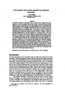
Figure 1. Algorithm overview using an example with p = 4 processes and n = 60 + 45 + 70 + 50 keys. the sorting permutation), which are then both locally and globally in sorted order. Assuming ascending order, this means that • ∀i ∈ [0, p), 0 ≤ k < l < ni : Ai [k] ≤ Ai [l] and
• ∀0 ≤ i < j < p, ki ∈ [0, ni ), kj ∈ [0, nj ) : Ai [ki ] ≤ Aj [kj ].
The parallel sorting algorithm comprises four steps, which are illustrated in Figure 1: 1. Local sorting 2. Exact splitter finding 3. Data redistribution 4. Local p-way merging The first step sorts all local arrays Ai in parallel using a sequential sorting algorithm. In Section 3.1, we will discuss criteria for the selection of a suitable algorithm, which may lead to choices different from what has been used in the literature so far at this stage. The second step, which constitutes the actual core of our work, identifies each splitter via a global binary search. Here, the main challenge lies in performing the binary search globally across data that is sorted only locally. While cutting the search space successively in halves is accomplished via a combination of local and global median selection, choosing either the upper or lower half requires determining the global rank of the selected median via a reduction operation across all processes. Once the splitters have been identified and the local arrays partitioned accordingly, the data is redistributed in a collective all-to-all communication operation during the third step. The fourth step finally merges the redistributed sorted partitions locally, resulting in a globally sorted overall sequence. In the following, we will explain each step in detail.
2010/12/22
s0 [
s1 rank 0
)[
rank 1
s2
...
)[
...
s p−2
s p−1
sp
)[ rank p−2 )[ rank p−1 )
Figure 2. Global partitioning of sorted sequence using splitters. 3.1 Local Sorting During the first step, all process-local arrays are sorted in parallel, with each individual array being sorted sequentially. Requiring no interaction among different processes, these operations can be performed independently from each other with a running time of O( np log np ) using an asymptotically optimal sorting algorithm. The well-known quicksort algorithm reaches this upper time bound only with a deterministic median selection, which is rather slow and therefore rarely used in practice. In contrast, the more prevalent randomized or median-of-three quicksort variants (e.g., the qsort() or sort algorithms from the libc or C++ STL, respectively) can yield this running time only on average. In these cases the actual performance not only depends on the number of elements but is also sensitive to the input data itself. In general, using such sensitive kernels with unpredictable running times in spite of constant numeric problem sizes in parallel applications can cause serious load imbalance, resulting in large implicit synchronization overhead during subsequent communication steps. Merge sort, on the contrary, never exceeds its upper bound running time, while being almost completely insensitive to the actual input data. That is, the performance is only influenced by the number of elements. Provided that all processes hold roughly the same number of elements and all processors can sort equally fast, all processes will accomplish this first step within the same time span – a desirable property for our parallel sorting algorithm. Another advantage of a straightforward merge sort implementation is its stability, that is, it maintains the relative order of elements with equal keys, thus enabling a stable parallel sorting algorithm. On the other hand, the extra memory consumed by the temporary buffer for the merge sub-step can be seen as a drawback, although in-place merging strategies exist in the literature [17]. We managed to tune our merge-sort implementation to be competitive to existing quicksort implementations within our algorithmic framework, making it much faster than the frequent outliers of quicksort, which become more dominant as the number of processes increases. Note also that the probability of bad choices in quicksort rises with an increasing number of processes. Therefore we strongly advise against using quicksort in any parallel application at larger scale because even a single slow process will degrade the overall performance. 3.2 Splitter Finding The most challenging part of our parallel sorting algorithm is to determine the exact splitting points. The splitters s0 , s1 , . . . , sp define a global partitioning of the overall sequence with two adjacent splitters delineating the partition assigned to a single process. This means that the process with rank i will eventually hold all elements in the range [si , si+1 ) (cf. Figure 2). In the rest of this paper, we assume the most common scenario, where the number of input elements ni equals the number of output elements. However, because this final partitioning is independent of ni (except that the total number of elements needs to stay constant), our algorithm can be easily extended to support a partitioning different from the initial distribution. To allow duplicate keys, each splitter consists of a key value and additionally an index representing the position relative to all elements matching the same key value. Since the outermost splitters s0 and sp reflect −∞ and +∞, they seem to be trivially defined and not worth further consideration. However, given that we search for the remaining splitters
4
only across the existing keys instead of searching their whole domain, we need the outermost splitters as starting point for our binary searches, initializing them with the global minimum and maximum of the key values, respectively. In addition, the index of s0 is set to 0 and the index of sp to the number of elements equal to this global maximum key. In our MPI-based implementation, this is accomplished using reductions across all processes using minimum, maximum, and summation as operators, as shown in the simplified pseudocode given in Listing 1. The remaining p − 1 splitters can be found by leveraging global binary searches. loc_min = A[0] glo_min = Allreduce(loc_min , OP_MIN) splitter[0] = loc_max = A[loc_n − 1] glo_max = Allreduce(loc_max , OP_MAX) loc_cnt = loc_n − num_less_than(A , loc_n , glo_max) glo_cnt = Allreduce(loc_cnt , OP_SUM) splitter[p] = target_cnt = Broadcast(loc_n , 0) for i = 1 to p − 1 splitter[i] = find_splitter(target_cnt , A , loc_n , splitter[0] , splitter[p]) target_cnt += Broadcast(loc_n , i) end for return splitter
Listing 1. Pseudocode for the splitter finding loop. The initial reductions as well as the communication overhead involved in the median selection (discussed later in this section) would not be necessary if we followed a naive approach, searching across the whole domain of key values. This would lead to O(log n′ ) binary search rounds where n′ corresponds to the range of the values to be searched, which can be moderate if the keys are smaller integer types but can also be high, for example, if keys are floating-point or big-integer types. However, we disqualified this approach also because it only works for certain key types and easily fails for other types like strings. Instead, we suggest a global binary search across the actual key values itself that cuts the search space into two halves, globally counts the number of elements in each of them, and proceeds with the half where the target count derived from the ni values resides until the desired splitter is found. With this approach, each of these splitter searches needs O(log n) rounds, where n reflects the total number of keys, independently of the range covered by their values. Each round consists of the following three sub-steps: (i) selecting a global median to split the search space, (ii) searching locally for this median to determine its local position, and (iii) counting globally all elements that are (a) less than and (b) less than or equal to this median using global reductions. The two counts (a, b) in the latter sub-step are needed in the presence of duplicate keys. In this case, the target count derived from the ni should reside in the interval delimited by those two values. At this point, either the desired splitter is found and the search is finished, or the search is continued to the left or to the right of the median value. More detailed information about this global binary search can be found within the non-recursive pseudocode given in Listing 2. The aggregate time complexity to find all exact splitting points amounts to O(p log2 n) because local binary search can be accomplished in time O(log np ), and parallel median selection (discussed next) as well as global summation can both be done in time O(log p) using reductions and broadcasts within tree-based communication graphs.
2010/12/22
/* [omitted handling of same key but different count] */ loop /* O(log n) rounds */ x = loc_n − num_greater_than(A , loc_n , min) y = num_less_than(A , loc_n , max) if x < y have_value = true loc_median = median(A , x , y) else have_value = false end if glo_median = sparse_median(loc_median , have_value) loc_cnt = num_less_than(A , loc_n , glo_median) a = Allreduce(loc_cnt , OP_SUM) if target_cnt < a max = glo_median continue loop end if loc_cnt = num_greater_than(A , loc_n , glo_median) b = Allreduce(loc_n − loc_cnt , OP_SUM) if target_cnt > b min = glo_median continue loop end if return end loop
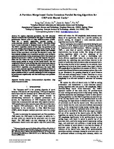
Listing 2. Pseudocode for a single splitter search. Due to the work of Han [18], we can presume that a parallel median algorithm exists with an optimal running time of O(log p). For all practical purposes however, it is sufficient to implement a potentially much simpler “approximate” median algorithm to find the splitters. Only the running time of this 2nd step is influenced by the choice of the selected value, not the correctness of the resulting exact splitting points. Thus an eligible method needs to globally agree upon one key value that splits the search range into two halves, which are not necessarily exact but nearly of the same size. We propose a median-of-3 reduction scheme within a complete ternary tree topology, like the example shown in Figure 3(a). Processes that correspond to inner nodes of such a tree receive the local median from two other processes (except for the last node in each round, which may receive less), determine the median of those values including the own value, and forward the result to the next level, where the same reduction procedure gets recursively ap≈ plied until a single result is selected. This final value x is a suitable approximation of the real median, and as such broadcasted to all participating processes. Because there is no identity element for comparisons, a sparse median selection procedure is needed that can handle dispensable processes without contributions to the median selection. This scenario occurs when the remaining number of local keys to be searched reaches zero on some but not all processes. Fortunately, an exclusive prefix sum followed by a sum reduction to all processes (alternatively a broadcast from the last process) and a single element redistribution (a.k.a. data shift) can be used to transform such a sparse algorithm back into a dense one, which subsequently proceeds as explained before. This transformation does not overbalance the O(log p) running time, while alternatives like creating a new communicator (e.g., using MPI Comm split) would inflate the running time to Ω(p). Another noteworthy approach to implement the median algorithm creates a data structure holding O(log n) values, each consisting of a key and a count. A cell at position i (0 ≤ i ≤ ⌊log n⌋) holds either 0, 1, or 2 key values representing an intermediate median of 2i elements. An MPI user-defined data type is created for this data structure, and a user-defined operation needs to be imple-
5
mented to combine two such structures into a single one. Such a combination proceeds from the lowest to the highest cell position, and puts all key values from the same position together. Whenever the number of gathered values exceeds two, they are replaced by their median value, which is put back into the corresponding cell(s) of the accumulated size. This is comparable to the procedure for adding big integers digit by digit while dealing with the carry. Once everything is set up, the data structure is initialized with the local median value, and a single MPI Allreduce operation is used to accomplish the complete median selection procedure. While this can be beneficial on some architectures, for example when the MPI collective function is optimized for the underlying interconnection network, the additional combination overhead leads to a trivial running time of O(log 2 p), exceeding our targeted running time. Using a sparse representation of the data structure and clever techniques similar to recursive doubling, the running time can be improved to yield the intended running time again. However, due to space restrictions and non-generality issues we do not go into more details of this quite complex method and therefore stick to the first commended approach for the sparse median selection also for the evaluation. ≈ While such a median approximation x does not necessarily reflect the exact median, it is in practice very close to it. It can be shown (straightforward proof via induction) that the 2log3 n − 1 smallest as well as 2log3 n − 1 largest keys out of n = 3k (∀ k ∈ N and k > 0) keys will never be chosen as an approximate median. Indeed, based upon the vertex coloring/symbols given in Figure 3(a), it is even possible to construct such a worst case input for any number of input keys n. However, simulations with 2187, 6561 and 19683 random keys (corresponding to the same number of processes) substantiate the expectations in that the true median is picked with highest probability, and the likelihood that this algorithm returns a key further away from the median decreases exponentially with its distance to this median. Figure 3(b) shows a simulation with a true median of 1093, resulting in an expected distance to this median E(X) of merely 36.427. While the theoretically possible worst case split is 1 : 16, we never encountered more than a 1 : 1.9 split in trillions of executions in practice. We distance ourselves from using interpolation functions such as a weighted arithmetic mean value for several reasons. While this is very simple to compute and therefore extremely fast (e.g., a single Allreduce with sum as operation) compared to our slow median selection (which currently uses Exscan + Broadcast + data shift + median-of-3 reduction + Broadcast), it only works on computable keys (like floating point or integer values2 ). Thus our algorithm would loose its general applicability. Additionally, we discussed the quality of the selected approximation to the true median and therefore were able to give a complete running time analysis of our parallel sorting algorithm. But none of the referenced papers in Section 2 that used this computational shortcut to appear fast were able to do so. We decided not to sacrifice general applicability for the sake of a running time reduction by a factor of 5 in the splitter finding step. Instead, we believe that further optimizations of the more general median selection algorithm might eventually be able to achieve similar speedups. 3.3 Data Redistribution Once the exact splitters have been determined in step 3.2, all elements can be redistributed accordingly to their final destinations. In order to accomplish this task with a single complete data exchange operation, the necessary process-local send and receive lists have to 2 Nonetheless,
there are practical issues like integer overflows or nonassociativity of floating point numbers when adding and multiplying very small with very large values.
2010/12/22
1
2
3
4
5
6
7
8
9
∗
∗
?
∗
∗
∗
?
∗
∗
∗
∗
∗
However, due to the quadratic growth of cabling costs that is needed to obtain full bisection bandwidth, large supercomputers typically provide a much smaller bisection bandwidth. This negatively impacts the performance of any complete exchange operation. For supercomputer architectures, such as the Blue Gene/L or the Cray XT5, where every node is only linked to a constant number of neighbors (i.e., 6 in those three dimensional tori), the data exchange scales only according to O(p × np ), which equals the very poor O(n) performance. Other parallel sorting algorithms like parallel quicksort or parallel merge sort [21] need O(log p) or even O(log n) complete data exchanges. Although the proposed parallel sorting algorithm needs only one such exchange operation and therefore reduces the bandwidth requirements to an absolute minimum, the necessary complete data exchange can anyhow and easily become the main bottleneck. Since this problem is expected to become even more severe in the future, as system sizes increase further, we would like to encourage architectures aiming at a high effective bisection bandwidth.
∗
≈
less than x ≈
∗
equal to x
∗
greater than x
?
≈
≈
unrelated to x
∗ ≈
x
(a) Median-of-3 reduction tree 109 108 107
Frequency
106 105 104 103 102 101 100
xxxxxxxxxxx xxxxxxxxxxxxxxxxxxxxxxxxxxxxxxxxxxxxxxxxxxxxxxxxx xxxxxxxxxxx xxxxxxxxxxxxxxxxxxxxxxxxxxxxxxxxxxxxxxxxxxxxxxxxx xxxxxxxxxxx xxxxxxxxxxxxxxxxxxxxxxxxxxxxxxxxxxxxxxxxxxxxxxxxx xxxxxxxxxxx xxxxxxxxxxxxxxxxxxxxxxxxxxxxxxxxxxxxxxxxxxxxxxxxx xxxxxxxxxxx xxxxxxxxxxxxxxxxxxxxxxxxxxxxxxxxxxxxxxxxxxxxxxxxx xxxxxxxxxxx xxxxxxxxxxxxxxxxxxxxxxxxxxxxxxxxxxxxxxxxxxxxxxxxx xxxxxxxxxxx xxxxxxxxxxxxxxxxxxxxxxxxxxxxxxxxxxxxxxxxxxxxxxxxx xxxxxxxxxxx xxxxxxxxxxxxxxxxxxxxxxxxxxxxxxxxxxxxxxxxxxxxxxxxx xxxxxxxxxxx xxxxxxxxxxxxxxxxxxxxxxxxxxxxxxxxxxxxxxxxxxxxxxxxx xxxxxxxxxxx xxxxxxxxxxxxxxxxxxxxxxxxxxxxxxxxxxxxxxxxxxxxxxxxx xxxxxxxxxxx xxxxxxxxxxxxxxxxxxxxxxxxxxxxxxxxxxxxxxxxxxxxxxxxx xxxxxxxxxxx xxxxxxxxxxxxxxxxxxxxxxxxxxxxxxxxxxxxxxxxxxxxxxxxx xxxxxxxxxxx xxxxxxxxxxxxxxxxxxxxxxxxxxxxxxxxxxxxxxxxxxxxxxxxx xxxxxxxxxxx xxxxxxxxxxxxxxxxxxxxxxxxxxxxxxxxxxxxxxxxxxxxxxxxx xxxxxxxxxxx xxxxxxxxxxxxxxxxxxxxxxxxxxxxxxxxxxxxxxxxxxxxxxxxx xxxxxxxxxxx xxxxxxxxxxxxxxxxxxxxxxxxxxxxxxxxxxxxxxxxxxxxxxxxx xxxxxxxxxxx xxxxxxxxxxxxxxxxxxxxxxxxxxxxxxxxxxxxxxxxxxxxxxxxx xxxxxxxxxxx xxxxxxxxxxxxxxxxxxxxxxxxxxxxxxxxxxxxxxxxxxxxxxxxx xxxxxxxxxxx xxxxxxxxxxxxxxxxxxxxxxxxxxxxxxxxxxxxxxxxxxxxxxxxx xxxxxxxxxxx xxxxxxxxxxxxxxxxxxxxxxxxxxxxxxxxxxxxxxxxxxxxxxxxx xxxxxxxxxxx xxxxxxxxxxxxxxxxxxxxxxxxxxxxxxxxxxxxxxxxxxxxxxxxx xxxxxxxxxxx xxxxxxxxxxxxxxxxxxxxxxxxxxxxxxxxxxxxxxxxxxxxxxxxx xxxxxxxxxxx xxxxxxxxxxxxxxxxxxxxxxxxxxxxxxxxxxxxxxxxxxxxxxxxx xxxxxxxxxxx xxxxxxxxxxxxxxxxxxxxxxxxxxxxxxxxxxxxxxxxxxxxxxxxx xxxxxxxxxxx xxxxxxxxxxxxxxxxxxxxxxxxxxxxxxxxxxxxxxxxxxxxxxxxx xxxxxxxxxxx xxxxxxxxxxxxxxxxxxxxxxxxxxxxxxxxxxxxxxxxxxxxxxxxx xxxxxxxxxxx xxxxxxxxxxxxxxxxxxxxxxxxxxxxxxxxxxxxxxxxxxxxxxxxx xxxxxxxxxxx xxxxxxxxxxxxxxxxxxxxxxxxxxxxxxxxxxxxxxxxxxxxxxxxx xxxxxxxxxxx xxxxxxxxxxxxxxxxxxxxxxxxxxxxxxxxxxxxxxxxxxxxxxxxx xxxxxxxxxxx xxxxxxxxxxxxxxxxxxxxxxxxxxxxxxxxxxxxxxxxxxxxxxxxx xxxxxxxxxxx xxxxxxxxxxxxxxxxxxxxxxxxxxxxxxxxxxxxxxxxxxxxxxxxx xxxxxxxxxxx xxxxxxxxxxxxxxxxxxxxxxxxxxxxxxxxxxxxxxxxxxxxxxxxx xxxxxxxxxxx xxxxxxxxxxxxxxxxxxxxxxxxxxxxxxxxxxxxxxxxxxxxxxxxx xxxxxxxxxxx xxxxxxxxxxxxxxxxxxxxxxxxxxxxxxxxxxxxxxxxxxxxxxxxx xxxxxxxxxxx xxxxxxxxxxxxxxxxxxxxxxxxxxxxxxxxxxxxxxxxxxxxxxxxx xxxxxxxxxxx xxxxxxxxxxxxxxxxxxxxxxxxxxxxxxxxxxxxxxxxxxxxxxxxx xxxxxxxxxxx xxxxxxxxxxxxxxxxxxxxxxxxxxxxxxxxxxxxxxxxxxxxxxxxx xxxxxxxxxxx xxxxxxxxxxxxxxxxxxxxxxxxxxxxxxxxxxxxxxxxxxxxxxxxx xxxxxxxxxxx xxxxxxxxxxxxxxxxxxxxxxxxxxxxxxxxxxxxxxxxxxxxxxxxx xxxxxxxxxxx xxxxxxxxxxxxxxxxxxxxxxxxxxxxxxxxxxxxxxxxxxxxxxxxx xxxxxxxxxxx xxxxxxxxxxxxxxxxxxxxxxxxxxxxxxxxxxxxxxxxxxxxxxxxx xxxxxxxxxxx xxxxxxxxxxxxxxxxxxxxxxxxxxxxxxxxxxxxxxxxxxxxxxxxx xxxxxxxxxxx xxxxxxxxxxxxxxxxxxxxxxxxxxxxxxxxxxxxxxxxxxxxxxxxx xxxxxxxxxxx xxxxxxxxxxxxxxxxxxxxxxxxxxxxxxxxxxxxxxxxxxxxxxxxx xxxxxxxxxxx xxxxxxxxxxxxxxxxxxxxxxxxxxxxxxxxxxxxxxxxxxxxxxxxx xxxxxxxxxxx xxxxxxxxxxxxxxxxxxxxxxxxxxxxxxxxxxxxxxxxxxxxxxxxx xxxxxxxxxxx xxxxxxxxxxxxxxxxxxxxxxxxxxxxxxxxxxxxxxxxxxxxxxxxx xxxxxxxxxxx xxxxxxxxxxxxxxxxxxxxxxxxxxxxxxxxxxxxxxxxxxxxxxxxx xxxxxxxxxxx xxxxxxxxxxxxxxxxxxxxxxxxxxxxxxxxxxxxxxxxxxxxxxxxx xxxxxxxxxxx xxxxxxxxxxxxxxxxxxxxxxxxxxxxxxxxxxxxxxxxxxxxxxxxx xxxxxxxxxxx xxxxxxxxxxxxxxxxxxxxxxxxxxxxxxxxxxxxxxxxxxxxxxxxx xxxxxxxxxxx xxxxxxxxxxxxxxxxxxxxxxxxxxxxxxxxxxxxxxxxxxxxxxxxx xxxxxxxxxxx xxxxxxxxxxxxxxxxxxxxxxxxxxxxxxxxxxxxxxxxxxxxxxxxx xxxxxxxxxxx xxxxxxxxxxxxxxxxxxxxxxxxxxxxxxxxxxxxxxxxxxxxxxxxx xxxxxxxxxxx xxxxxxxxxxxxxxxxxxxxxxxxxxxxxxxxxxxxxxxxxxxxxxxxx xxxxxxxxxxx xxxxxxxxxxxxxxxxxxxxxxxxxxxxxxxxxxxxxxxxxxxxxxxxx xxxxxxxxxxx xxxxxxxxxxxxxxxxxxxxxxxxxxxxxxxxxxxxxxxxxxxxxxxxx xxxxxxxxxxx xxxxxxxxxxxxxxxxxxxxxxxxxxxxxxxxxxxxxxxxxxxxxxxxx xxxxxxxxxxx xxxxxxxxxxxxxxxxxxxxxxxxxxxxxxxxxxxxxxxxxxxxxxxxx xxxxxxxxxxx xxxxxxxxxxxxxxxxxxxxxxxxxxxxxxxxxxxxxxxxxxxxxxxxx xxxxxxxxxxx xxxxxxxxxxxxxxxxxxxxxxxxxxxxxxxxxxxxxxxxxxxxxxxxx xxxxxxxxxxx xxxxxxxxxxxxxxxxxxxxxxxxxxxxxxxxxxxxxxxxxxxxxxxxx xxxxxxxxxxx xxxxxxxxxxxxxxxxxxxxxxxxxxxxxxxxxxxxxxxxxxxxxxxxx xxxxxxxxxxx xxxxxxxxxxxxxxxxxxxxxxxxxxxxxxxxxxxxxxxxxxxxxxxxx xxxxxxxxxxx xxxxxxxxxxxxxxxxxxxxxxxxxxxxxxxxxxxxxxxxxxxxxxxxx xxxxxxxxxxx xxxxxxxxxxxxxxxxxxxxxxxxxxxxxxxxxxxxxxxxxxxxxxxxx xxxxxxxxxxx xxxxxxxxxxxxxxxxxxxxxxxxxxxxxxxxxxxxxxxxxxxxxxxxx xxxxxxxxxxx xxxxxxxxxxxxxxxxxxxxxxxxxxxxxxxxxxxxxxxxxxxxxxxxx xxxxxxxxxxx xxxxxxxxxxxxxxxxxxxxxxxxxxxxxxxxxxxxxxxxxxxxxxxxx xxxxxxxxxxx xxxxxxxxxxxxxxxxxxxxxxxxxxxxxxxxxxxxxxxxxxxxxxxxx xxxxxxxxxxx xxxxxxxxxxxxxxxxxxxxxxxxxxxxxxxxxxxxxxxxxxxxxxxxx xxxxxxxxxxx xxxxxxxxxxxxxxxxxxxxxxxxxxxxxxxxxxxxxxxxxxxxxxxxx xxxxxxxxxxx xxxxxxxxxxxxxxxxxxxxxxxxxxxxxxxxxxxxxxxxxxxxxxxxx xxxxxxxxxxx xxxxxxxxxxxxxxxxxxxxxxxxxxxxxxxxxxxxxxxxxxxxxxxxx xxxxxxxxxxx xxxxxxxxxxxxxxxxxxxxxxxxxxxxxxxxxxxxxxxxxxxxxxxxx xxxxxxxxxxx xxxxxxxxxxxxxxxxxxxxxxxxxxxxxxxxxxxxxxxxxxxxxxxxx xxxxxxxxxxx xxxxxxxxxxxxxxxxxxxxxxxxxxxxxxxxxxxxxxxxxxxxxxxxx xxxxxxxxxxx xxxxxxxxxxxxxxxxxxxxxxxxxxxxxxxxxxxxxxxxxxxxxxxxx xxxxxxxxxxx xxxxxxxxxxxxxxxxxxxxxxxxxxxxxxxxxxxxxxxxxxxxxxxxx xxxxxxxxxxx xxxxxxxxxxxxxxxxxxxxxxxxxxxxxxxxxxxxxxxxxxxxxxxxx xxxxxxxxxxx xxxxxxxxxxxxxxxxxxxxxxxxxxxxxxxxxxxxxxxxxxxxxxxxx xxxxxxxxxxx xxxxxxxxxxxxxxxxxxxxxxxxxxxxxxxxxxxxxxxxxxxxxxxxx xxxxxxxxxxx xxxxxxxxxxxxxxxxxxxxxxxxxxxxxxxxxxxxxxxxxxxxxxxxx xxxxxxxxxxx xxxxxxxxxxxxxxxxxxxxxxxxxxxxxxxxxxxxxxxxxxxxxxxxx xxxxxxxxxxx xxxxxxxxxxxxxxxxxxxxxxxxxxxxxxxxxxxxxxxxxxxxxxxxx xxxxxxxxxxx xxxxxxxxxxxxxxxxxxxxxxxxxxxxxxxxxxxxxxxxxxxxxxxxx xxxxxxxxxxx xxxxxxxxxxxxxxxxxxxxxxxxxxxxxxxxxxxxxxxxxxxxxxxxx xxxxxxxxxxx xxxxxxxxxxxxxxxxxxxxxxxxxxxxxxxxxxxxxxxxxxxxxxxxx xxxxxxxxxxx xxxxxxxxxxxxxxxxxxxxxxxxxxxxxxxxxxxxxxxxxxxxxxxxx xxxxxxxxxxx xxxxxxxxxxxxxxxxxxxxxxxxxxxxxxxxxxxxxxxxxxxxxxxxx xxxxxxxxxxx xxxxxxxxxxxxxxxxxxxxxxxxxxxxxxxxxxxxxxxxxxxxxxxxx
250
500
750
xxxxxxxxxxxxxxxxxxxxxxxxxxxxxxxxxxxxxxxxxxxxxxxxx xxxxxxxxxxx xxxxxxxxxxxxxxxxxxxxxxxxxxxxxxxxxxxxxxxxxxxxxxxxx xxxxxxxxxxx xxxxxxxxxxxxxxxxxxxxxxxxxxxxxxxxxxxxxxxxxxxxxxxxx xxxxxxxxxxx xxxxxxxxxxxxxxxxxxxxxxxxxxxxxxxxxxxxxxxxxxxxxxxxx xxxxxxxxxxx xxxxxxxxxxxxxxxxxxxxxxxxxxxxxxxxxxxxxxxxxxxxxxxxx xxxxxxxxxxx xxxxxxxxxxxxxxxxxxxxxxxxxxxxxxxxxxxxxxxxxxxxxxxxx xxxxxxxxxxx xxxxxxxxxxxxxxxxxxxxxxxxxxxxxxxxxxxxxxxxxxxxxxxxx xxxxxxxxxxx xxxxxxxxxxxxxxxxxxxxxxxxxxxxxxxxxxxxxxxxxxxxxxxxx xxxxxxxxxxx xxxxxxxxxxxxxxxxxxxxxxxxxxxxxxxxxxxxxxxxxxxxxxxxx xxxxxxxxxxx xxxxxxxxxxxxxxxxxxxxxxxxxxxxxxxxxxxxxxxxxxxxxxxxx xxxxxxxxxxx xxxxxxxxxxxxxxxxxxxxxxxxxxxxxxxxxxxxxxxxxxxxxxxxx xxxxxxxxxxx xxxxxxxxxxxxxxxxxxxxxxxxxxxxxxxxxxxxxxxxxxxxxxxxx xxxxxxxxxxx xxxxxxxxxxxxxxxxxxxxxxxxxxxxxxxxxxxxxxxxxxxxxxxxx xxxxxxxxxxx xxxxxxxxxxxxxxxxxxxxxxxxxxxxxxxxxxxxxxxxxxxxxxxxx xxxxxxxxxxx xxxxxxxxxxxxxxxxxxxxxxxxxxxxxxxxxxxxxxxxxxxxxxxxx xxxxxxxxxxx xxxxxxxxxxxxxxxxxxxxxxxxxxxxxxxxxxxxxxxxxxxxxxxxx xxxxxxxxxxx xxxxxxxxxxxxxxxxxxxxxxxxxxxxxxxxxxxxxxxxxxxxxxxxx xxxxxxxxxxx xxxxxxxxxxxxxxxxxxxxxxxxxxxxxxxxxxxxxxxxxxxxxxxxx xxxxxxxxxxx xxxxxxxxxxxxxxxxxxxxxxxxxxxxxxxxxxxxxxxxxxxxxxxxx xxxxxxxxxxx xxxxxxxxxxxxxxxxxxxxxxxxxxxxxxxxxxxxxxxxxxxxxxxxx xxxxxxxxxxx xxxxxxxxxxxxxxxxxxxxxxxxxxxxxxxxxxxxxxxxxxxxxxxxx xxxxxxxxxxx xxxxxxxxxxxxxxxxxxxxxxxxxxxxxxxxxxxxxxxxxxxxxxxxx xxxxxxxxxxx xxxxxxxxxxxxxxxxxxxxxxxxxxxxxxxxxxxxxxxxxxxxxxxxx xxxxxxxxxxx xxxxxxxxxxxxxxxxxxxxxxxxxxxxxxxxxxxxxxxxxxxxxxxxx xxxxxxxxxxx xxxxxxxxxxxxxxxxxxxxxxxxxxxxxxxxxxxxxxxxxxxxxxxxx xxxxxxxxxxx xxxxxxxxxxxxxxxxxxxxxxxxxxxxxxxxxxxxxxxxxxxxxxxxx xxxxxxxxxxx xxxxxxxxxxxxxxxxxxxxxxxxxxxxxxxxxxxxxxxxxxxxxxxxx xxxxxxxxxxx xxxxxxxxxxxxxxxxxxxxxxxxxxxxxxxxxxxxxxxxxxxxxxxxx xxxxxxxxxxx xxxxxxxxxxxxxxxxxxxxxxxxxxxxxxxxxxxxxxxxxxxxxxxxx xxxxxxxxxxx xxxxxxxxxxxxxxxxxxxxxxxxxxxxxxxxxxxxxxxxxxxxxxxxx xxxxxxxxxxx xxxxxxxxxxxxxxxxxxxxxxxxxxxxxxxxxxxxxxxxxxxxxxxxx xxxxxxxxxxx xxxxxxxxxxxxxxxxxxxxxxxxxxxxxxxxxxxxxxxxxxxxxxxxx xxxxxxxxxxx xxxxxxxxxxxxxxxxxxxxxxxxxxxxxxxxxxxxxxxxxxxxxxxxx xxxxxxxxxxx xxxxxxxxxxxxxxxxxxxxxxxxxxxxxxxxxxxxxxxxxxxxxxxxx xxxxxxxxxxx xxxxxxxxxxxxxxxxxxxxxxxxxxxxxxxxxxxxxxxxxxxxxxxxx xxxxxxxxxxx xxxxxxxxxxxxxxxxxxxxxxxxxxxxxxxxxxxxxxxxxxxxxxxxx xxxxxxxxxxx xxxxxxxxxxxxxxxxxxxxxxxxxxxxxxxxxxxxxxxxxxxxxxxxx xxxxxxxxxxx xxxxxxxxxxxxxxxxxxxxxxxxxxxxxxxxxxxxxxxxxxxxxxxxx xxxxxxxxxxx xxxxxxxxxxxxxxxxxxxxxxxxxxxxxxxxxxxxxxxxxxxxxxxxx xxxxxxxxxxx xxxxxxxxxxxxxxxxxxxxxxxxxxxxxxxxxxxxxxxxxxxxxxxxx xxxxxxxxxxx xxxxxxxxxxxxxxxxxxxxxxxxxxxxxxxxxxxxxxxxxxxxxxxxx xxxxxxxxxxx xxxxxxxxxxxxxxxxxxxxxxxxxxxxxxxxxxxxxxxxxxxxxxxxx xxxxxxxxxxx xxxxxxxxxxxxxxxxxxxxxxxxxxxxxxxxxxxxxxxxxxxxxxxxx xxxxxxxxxxx xxxxxxxxxxxxxxxxxxxxxxxxxxxxxxxxxxxxxxxxxxxxxxxxx xxxxxxxxxxx xxxxxxxxxxxxxxxxxxxxxxxxxxxxxxxxxxxxxxxxxxxxxxxxx xxxxxxxxxxx xxxxxxxxxxxxxxxxxxxxxxxxxxxxxxxxxxxxxxxxxxxxxxxxx xxxxxxxxxxx xxxxxxxxxxxxxxxxxxxxxxxxxxxxxxxxxxxxxxxxxxxxxxxxx xxxxxxxxxxx xxxxxxxxxxxxxxxxxxxxxxxxxxxxxxxxxxxxxxxxxxxxxxxxx xxxxxxxxxxx xxxxxxxxxxxxxxxxxxxxxxxxxxxxxxxxxxxxxxxxxxxxxxxxx xxxxxxxxxxx xxxxxxxxxxxxxxxxxxxxxxxxxxxxxxxxxxxxxxxxxxxxxxxxx xxxxxxxxxxx xxxxxxxxxxxxxxxxxxxxxxxxxxxxxxxxxxxxxxxxxxxxxxxxx xxxxxxxxxxx xxxxxxxxxxxxxxxxxxxxxxxxxxxxxxxxxxxxxxxxxxxxxxxxx xxxxxxxxxxx xxxxxxxxxxxxxxxxxxxxxxxxxxxxxxxxxxxxxxxxxxxxxxxxx xxxxxxxxxxx xxxxxxxxxxxxxxxxxxxxxxxxxxxxxxxxxxxxxxxxxxxxxxxxx xxxxxxxxxxx xxxxxxxxxxxxxxxxxxxxxxxxxxxxxxxxxxxxxxxxxxxxxxxxx xxxxxxxxxxx xxxxxxxxxxxxxxxxxxxxxxxxxxxxxxxxxxxxxxxxxxxxxxxxx xxxxxxxxxxx xxxxxxxxxxxxxxxxxxxxxxxxxxxxxxxxxxxxxxxxxxxxxxxxx xxxxxxxxxxx xxxxxxxxxxxxxxxxxxxxxxxxxxxxxxxxxxxxxxxxxxxxxxxxx xxxxxxxxxxx xxxxxxxxxxxxxxxxxxxxxxxxxxxxxxxxxxxxxxxxxxxxxxxxx xxxxxxxxxxx xxxxxxxxxxxxxxxxxxxxxxxxxxxxxxxxxxxxxxxxxxxxxxxxx xxxxxxxxxxx xxxxxxxxxxxxxxxxxxxxxxxxxxxxxxxxxxxxxxxxxxxxxxxxx xxxxxxxxxxx xxxxxxxxxxxxxxxxxxxxxxxxxxxxxxxxxxxxxxxxxxxxxxxxx xxxxxxxxxxx xxxxxxxxxxxxxxxxxxxxxxxxxxxxxxxxxxxxxxxxxxxxxxxxx xxxxxxxxxxx xxxxxxxxxxxxxxxxxxxxxxxxxxxxxxxxxxxxxxxxxxxxxxxxx xxxxxxxxxxx xxxxxxxxxxxxxxxxxxxxxxxxxxxxxxxxxxxxxxxxxxxxxxxxx xxxxxxxxxxx xxxxxxxxxxxxxxxxxxxxxxxxxxxxxxxxxxxxxxxxxxxxxxxxx xxxxxxxxxxx xxxxxxxxxxxxxxxxxxxxxxxxxxxxxxxxxxxxxxxxxxxxxxxxx xxxxxxxxxxx xxxxxxxxxxxxxxxxxxxxxxxxxxxxxxxxxxxxxxxxxxxxxxxxx xxxxxxxxxxx xxxxxxxxxxxxxxxxxxxxxxxxxxxxxxxxxxxxxxxxxxxxxxxxx xxxxxxxxxxx xxxxxxxxxxxxxxxxxxxxxxxxxxxxxxxxxxxxxxxxxxxxxxxxx xxxxxxxxxxx xxxxxxxxxxxxxxxxxxxxxxxxxxxxxxxxxxxxxxxxxxxxxxxxx xxxxxxxxxxx xxxxxxxxxxxxxxxxxxxxxxxxxxxxxxxxxxxxxxxxxxxxxxxxx xxxxxxxxxxx xxxxxxxxxxxxxxxxxxxxxxxxxxxxxxxxxxxxxxxxxxxxxxxxx xxxxxxxxxxx xxxxxxxxxxxxxxxxxxxxxxxxxxxxxxxxxxxxxxxxxxxxxxxxx xxxxxxxxxxx xxxxxxxxxxxxxxxxxxxxxxxxxxxxxxxxxxxxxxxxxxxxxxxxx xxxxxxxxxxx xxxxxxxxxxxxxxxxxxxxxxxxxxxxxxxxxxxxxxxxxxxxxxxxx xxxxxxxxxxx xxxxxxxxxxxxxxxxxxxxxxxxxxxxxxxxxxxxxxxxxxxxxxxxx xxxxxxxxxxx xxxxxxxxxxxxxxxxxxxxxxxxxxxxxxxxxxxxxxxxxxxxxxxxx xxxxxxxxxxx xxxxxxxxxxxxxxxxxxxxxxxxxxxxxxxxxxxxxxxxxxxxxxxxx xxxxxxxxxxx xxxxxxxxxxxxxxxxxxxxxxxxxxxxxxxxxxxxxxxxxxxxxxxxx xxxxxxxxxxx xxxxxxxxxxxxxxxxxxxxxxxxxxxxxxxxxxxxxxxxxxxxxxxxx xxxxxxxxxxx xxxxxxxxxxxxxxxxxxxxxxxxxxxxxxxxxxxxxxxxxxxxxxxxx xxxxxxxxxxx xxxxxxxxxxxxxxxxxxxxxxxxxxxxxxxxxxxxxxxxxxxxxxxxx xxxxxxxxxxx xxxxxxxxxxxxxxxxxxxxxxxxxxxxxxxxxxxxxxxxxxxxxxxxx xxxxxxxxxxx xxxxxxxxxxxxxxxxxxxxxxxxxxxxxxxxxxxxxxxxxxxxxxxxx xxxxxxxxxxx xxxxxxxxxxxxxxxxxxxxxxxxxxxxxxxxxxxxxxxxxxxxxxxxx xxxxxxxxxxx xxxxxxxxxxxxxxxxxxxxxxxxxxxxxxxxxxxxxxxxxxxxxxxxx xxxxxxxxxxx xxxxxxxxxxxxxxxxxxxxxxxxxxxxxxxxxxxxxxxxxxxxxxxxx xxxxxxxxxxx xxxxxxxxxxxxxxxxxxxxxxxxxxxxxxxxxxxxxxxxxxxxxxxxx xxxxxxxxxxx xxxxxxxxxxxxxxxxxxxxxxxxxxxxxxxxxxxxxxxxxxxxxxxxx xxxxxxxxxxx xxxxxxxxxxxxxxxxxxxxxxxxxxxxxxxxxxxxxxxxxxxxxxxxx xxxxxxxxxxx
1000 1250 Position of the Approximative Median
1500
1750
3.4 p-way Merging
2000
(b) 244 billion approximations with 2187 elements showing the areas for impossible (crosshatch) and never encountered results
Figure 3. Median reduction scheme and simulation of quality.
be prepared. All information for the send lists, consisting of p displacement and p count values, can be assembled by utilizing O(p) local binary searches followed by global prefix summations (e.g., MPI Scan with MPI SUM as operation), to account for duplicate keys. The corresponding process-local receive lists can be derived directly from these send lists using a regular complete exchange of those O(p) values per process (e.g., by invoking MPI Alltoall). Now everything is setup to finally redistribute the actual user data within a single but complete data exchange operation, like the irregular MPI Alltoallv collective. This is the only step where complete elements (i.e., keys and their potentially attached information) are communicated between processes. Because the data in the send buffer is not needed anymore, it could be replaced by the received data. Unfortunately, there is no “in place” option for the general MPI Alltoallv functionality with differing send and receive lists3 . Thus our current implement needs a second buffer just for the data reception. Fortunately, some recent developments explained in [19] and [20] suggest that it is possible to implement such a generic (i.e., non-symmetric) “in place” variant of an irregular and complete data exchange operation. Assuming an underlying interconnection network that provides full bisection bandwidth and therefore enables simultaneous pairwise communication, the running time of the pure data redistribution can be done in time O( np ). Together with the O(p) local binary searches and global prefix summations, each working in O(log np ) and O(log p) time respectively, the total running time of this third step of our parallel sorting algorithm becomes O( np + p log n). 3 Version 2.2 of the MPI standard includes the “in place” option for MPI Alltoallv, but the wording only covers the simpler symmetric variant.
6
After the previous data redistribution step, all elements reside at the correct processing elements. To conclude the parallel sorting algorithm, a process-local operation is needed that brings the elements into a sorted order. One might be tempted to apply a normal sorting operation as we did in the first step. However, because the data is already arranged in at most p sorted pieces, this approach would perform too much work and could cut the overall parallel efficiency in half. A multi-way merge operation, often used in the context of file-based sorting algorithms, accomplishes this last task by merging the O(p) pre-sorted pieces into the final sorted sequence. We propose to use a binary min-heap data structure capable of holding p elements, each consisting of a key and two index values. A new heap element is created for each pre-sorted piece and inserted into this heap. Its key is initialized according to the first entry of the corresponding piece, and the starting position as well as the end of this piece is assigned to the two index values. Once the heap is built, O( np ) extract-min operations are eventually utilized to copy all user elements in ascending order into a second buffer. The starting index of a heap element is increased after each such extraction. As long as the associated end index has not been reached, the key is updated according to the next user element and the heap element is inserted back into the heap structure. Given that each heap operation works in time O(log p), this approach yields the asymptotically optimal running time of O( np log p). An alternative approach could utilize a bottom-up variant of the merge sort algorithm. However, as opposed to the full sorting algorithm that starts merging single-element arrays, it commences at a later stage by merging the larger pre-sorted pieces. Both approaches accomplish the p-way merging task and both can be implemented to be stable. The min-heap solution spends O(log p) time per element operating within the small heap structure of size O(p) whereas each of the O( np ) user elements is only moved exactly once, laying the foundations for exploiting CPU caches very well. This gives a performance advantage on moderate-scale parallel architectures such as common cluster systems. On the other hand, the merge sort solution can again be made to work “in place” just like in step 3.1. Since we currently need a temporary buffer anyway because of the complete data exchange, we have chosen the cache-friendly min-heap approach for our evaluation. Last but not least, there still might be a rationale for using a complete sorting algorithm in this step, for example, if there exists a very fast sequential sorting implementation, such as an optimized version for GPUs, but no equally fast p-way merge operation. So whenever the best merge operation would perform worse than a complete sort, one might consider just applying the latter one.
2010/12/22
3.5 Algorithm Summary All four steps of our parallel sorting algorithm are visually represented in Figure 1 for a total of 225 elements that are unequally distributed among 4 processes. Each individual key value is illustrated by the height of the bars. The top most row shows the initial array contents for each process, which are filled with random values at the beginning. During the first step, these elements are locally sorted using merge sort. Afterwards, the resulting array contents show monotonically increasing key values at the individual ranks. The second step finds all 5 exact splitting points, drawn as red vertical lines in the middle row. The complete data exchange operation in step 3 moves all elements to their final destination process. This bandwidth-intensive all-to-all communication operation is indicated by the arrows. A p-way merging operation completes the parallel sorting algorithm by bringing the resulting pre-sorted pieces into the final sorted order. At the end, all elements in the bottom row are globally in sorted order. For completeness, the splitters that are found in the second step are shown again in the last row, matching the initial objective given in Figure 2. The following table summarizes all four steps together with the corresponding running times. 1st step 2nd step 3rd step 4th step
local sorting global splitter finding global data redistribution local p-way merging
O( np log np ) O(p log2 n) O( np + p log n) O( np log p)
The total running time of this parallel sorting algorithm is therefore O( np log n+p log 2 n). Considering only comparison-based approaches, an optimal parallel sorting algorithm with p processes runs in time O( np log n) because optimal sequential sorting algorithms are bounded by O(n log n). The presented algorithm is therefore asymptotically optimal as long as O(p2 ) ≤ O( logn n ). Assuming a fixed number of elements √ per process c, our sorting algorithm scales as long as c ≥ O( n log n ).
4. Example To further improve upon the understanding of our parallel sorting algorithm, a detailed example will be provided in this section. Randomly chosen prime numbers between 10 and 99 form the input data, which shall be sorted in parallel using p = 4 processes. For best performance, these n = 40 elements are equally distributed across all processes, thus giving ni = 10 ∀ 0 ≤ i < 4 with the following initial array contents Ai . rank rank rank rank
0: 1: 2: 3:
47 71 37 11
, , , ,
23 71 47 97
, , , ,
29 13 43 13
, , , ,
79 13 53 61
, , , ,
83 97 59 29
, , , ,
79 37 73 83
, , , ,
47 97 53 47
, , , ,
59 73 13 89
, , , ,
67 23 17 67
, , , ,
31 41 43 11
Each process starts by sorting its own local array in ascending order, yielding the following array contents after the 1st step. 0: 1: 2: 3:
23 13 13 11
, , , ,
29 13 17 11
, , , ,
31 23 37 13
, , , ,
47 37 43 29
, , , ,
47 41 43 47
, , , ,
59 71 47 61
, , , ,
67 71 53 67
, , , ,
79 73 53 83
, , , ,
79 97 59 89
, , , ,
s0 = // s4 = //
To find splitter s1 , we note that the first process with rank 0 holds 10 elements. Therefore, exactly 10 elements in the final sorted sequence must be located in the range covered by [s0 , s1 ). Because s0 with key 11 globally exists only twice and s4 with key 97 exists only three times, neither of both known keys can already fulfill this target count. So we initiate a global binary search for a key larger than 11 and smaller than 97 that satisfies a target count of 10. First, we determine the global median4 of all elements between 11 and 97, which is 47. Using local binary searches, we can essentially “count” the number of elements with respect to this median. Reducing these local counts into a global sum reveals that there are in total 17 smaller elements, which is too large for our target count of 10. Continuing the global binary search within the lower key range (11, 47) with the next median 23 gives 7 smaller elements and 2 equal elements, which is quite close but still one element too small. Therefore the splitter must be located somewhere in the upper halve (23, 47). The median there is 37 and turns up 12 smaller elements, making it slightly too large. Note that not all processes contribute elements to the next median finding step in the lower key range (23, 37). The resulting median value of 29 globally causes 9 elements to be smaller, 2 elements to be equal and 29 elements to be greater. So finally we found s1 with a key equal to this median value of 29 and an index value of 1, because there are 10 elements before this splitting point. The next splitter s2 is found in a similar fashion by adding the number of elements at rank 1 to the present target count. A following global binary search tries to find a splitter preceded by these 20 elements. Luckily, the first median value of 47 from the search range (11, 97) results in 17 elements that are smaller but additionally 4 elements that are equal to it. Since 20 < 17 + 4, we already found a suitable key for s2 and the corresponding index value needs to be 3. Our search for the last remaining splitter s3 proceeds with a target count of 30 and successively examines the ranges (11, 97) and (47, 97). The second median value of 71 makes a total of 28 smaller elements and 2 equal elements. Therefore s3 = serves as a suitable splitter after 30 global elements. However, depending on the actual implementation and the selected median values, note that it is also possible for s3 to end up having a key of 73 and an index value of 0. Both variants of s3 represent the exact same splitting point, merely expressed in two different ways. s1 = // comparison keys: 47, 23, 37, 29 s2 = // comparison keys: 47 s3 = // comparison keys: 47, 71
4.1 Local Sorting
rank rank rank rank
array position and the local maximum given by the last element in the array. The corresponding index value for the first splitter is always defined to be zero, and becomes three for the last splitter because the maximum 97 globally exists three times.
4.3 Data Redistribution Now that we have all necessary splitters, they are used to split the process-local arrays up. The only difficulty here lies in the handling of duplicate keys. For example, splitter s1 has a key value of 29 and an index of 1. Since both rank 0 and rank 3 have one element with this key, they need to know if the splitting needs to be done before or after this element5 . A so-called exclusive prefix sum (a.k.a. scan,
83 97 73 97
4.2 Splitter Finding Finding the exact splitting points s0 , s1 , s2 , s3 and s4 is the most challenging part. The keys of the outermost splitters s0 and s4 represent the global minimum and maximum key value respectively. These can be derived from the local minimum residing at the first
7
4 Remember: an arbitrary
element close to the median, which bisects a given sequence nearly equally, would be sufficient. 5 If there are multiple equal elements on a process, splitting can also happen anywhere between the first and last occurrence of elements with this key.
2010/12/22
prefix reduction or partial sum) determines the number of elements with the same key on all processes before the inquiring process. All processes simply provide their number of elements with the related key as input: ⇒. As a result, rank 0 knows that it has to split after this element because it is the first processor having this key, and rank 3 knows that it needs to split before this element because there is another process already handling the one element with this key. The local splitting of the arrays looks as follows. rank rank rank rank
0: 1: 2: 3:
23 13 13 11
, , , ,
29 13 17 11
| , | ,
31 23 37 13
, | , |
47 37 43 29
, , , |
47 41 43 47
| | , ,
59 71 47 61
, , | ,
67 71 53 67
| | , |
79 73 53 83
, , , ,
79 97 59 89
, , | ,
83 97 73 97
The first process notices that the first two elements need to be moved to itself, the next three elements to rank 1, the next two elements to rank 2, and the last three elements to the last process. All other processes also know to whom to send their elements. If all processes scatter this send information to all processes, then everyone grasps the complete receive information including where to receive the elements. So we can finally accomplish the complete data exchange, resulting in the following array contents. rank rank rank rank
0: 1: 2: 3:
23 31 59 79
, , , ,
29 47 67 79
| , | ,
13 47 71 83
, | , |
13 37 71 73
, , | ,
23 41 53 97
| | , ,
13 37 53 97
, , , |
17 43 59 73
| , | |
11 43 47 83
, , , ,
11 47 61 89
, | , ,
13 29 67 97
13 31 59 73
, , , ,
13 37 67 79
, , , ,
23 41 71 79
, , , ,
23 47 71 83
, , | ,
29 47 47 97
| | , ,
11 29 53 97
, , , |
11 37 53 73
, , , ,
13 43 59 83
, , , ,
13 43 61 89
, , , ,
17 47 67 97
rank rank rank rank
0: 1: 2: 3:
11 29 47 73
, , , ,
11 31 53 73
, , , ,
13 37 53 79
, , , ,
13 37 59 79
, , , ,
13 41 59 83
, , , ,
13 43 61 83
, , , ,
17 43 67 89
, , , ,
23 47 67 97
, , , ,
23 47 71 97
, , , ,
29 47 71 97
Tmergesort (n) = c · n · log2 n
resulting in a c between 14.4 and 13.9 for our first architecture. Plotting several of such derived c values in a logarithmic scale starting with 131 thousand elements up to 402 million elements clearly shows a linear trend downwards. We assume that this behaviour can be explained with cache utilization. The sequential performance prediction will thus fit a linear function c(2x ) = y = a · x + b to the measured results. The outcome will be merged with the first formula resulting in Once the sequential sorting performance can be predicted accurately, it will be used to calculate the achieved parallel efficiency E(n, p) according to the formula
Almost completed, every process holds the correct elements after the previous step. The pre-sorted pieces only need to be merged into a final sorted sequence. Since there are four processes, applying two bottom-up merge steps can accomplish this task. 0: 1: 2: 3:
To determine the parallel efficiency of our parallel sorting algorithm, we need to know the running time of the fastest sequential sorting algorithm. Since we were able to tune our merge sort implementation to be competitive to best case runs of existing quicksort implementations, we use this as a basis for the comparisons. However, currently there are no machines with terabytes of shared memory, which is the reason why we cannot just measure the sorting time for data sets at these sizes. Instead we need to be able to accurately predict the performance at this scale. As we discussed in the introduction, the theoretical runtime of merge sort for n elements is Θ(n log n). And indeed, the measured running time (given in nanoseconds) can be relatively well estimated using the formula
Tseq sort (n) = (a · log n + b) · n · log2 n
4.4 p-way Merging
rank rank rank rank
5.1 Sequential Performance
As demonstrated in this example, the parallel sorting algorithm correctly placed all elements in a globally ascending order.
5. Implementation and Results Our implementation of the presented parallel sorting algorithm is completely written in the ANSI-C language and only uses a Message Passing Interface library to accomplish the communication between the processes. For this reason, it is at the same time very portable and highly efficient, especially when used together with the vendor-tuned MPI implementation and compiler for the parallel computer architecture. We use merge sort for the local sorting step, and the native MPI Alltoallv operation of the underlying MPI for the data redistribution. The splitter finding step implements the sparse median selection procedure (using amongst other collectives MPI Exscan), and the p-way merge is build upon the presented min-heap approach. Since the median selection is also a collective operation (although not part of the MPI standard), our parallel sorting algorithm solely uses collective operations within a single communicator (i.e., MPI COMM WORLD). Thus, except for our median implementation, no point-to-point communication operations are used. The more sophisticated approaches would additionally require user-defined reduction operations and complex user-defined data types.
8
E(n, p) =
Tseq sort (n) p · Tpar sort (n, p)
5.2 Juropa “Juropa” is an InfiniBand cluster at the Supercomputing Center in J¨ulich/Germany with 2208 nodes, each equipped with two Intel Xeon X5570 (Nehalem-EP) quad-core processors running at 2.93 GHz and 24 GiB of memory. The sequential sorting performance on this architecture can be predicted using c(2x ) = 14.9153 − 0.0289 · x with high accuracy. The difference of this prediction compared to the actual measured performance was always less than 1.1%. Figure 4 shows the performance of our implementation of the presented parallel sorting algorithm, running in a weak scaling mode on up to 512 compute nodes6 . Using the sequential performance prediction, we have calculated the achieved parallel efficiency, which is given as number in percent above each bar. Up to 384 processes, the parallel efficiency is always above 97%. Afterwards it slowly decreases to 82.1% for the largest run with 1024 processes. Due to the enormous memory required by the InfiniBand layer in the MPI library, we only used 2 MPI processes per node and 671, 088, 640 elements per process. As can be seen, the data redistribution is not the bottleneck within this scale in this tightly coupled cluster system, which uses a Fat Tree topology. However, the memory requirements are becoming a serious problem at this scale, even inhibiting larger runs. Therefore an alternative but memory-economic MPI Alltoallv implementation (even if it is slower) would help to scale further. 5.3 Jugene “Jugene” is a Blue Gene/P installation at the Supercomputing Center in J¨ulich/Germany consisting of 72 racks with 32 nodecards 6 No
run for 2 MPI processes can be shown, because the MPI Alltoallv implementation provided by the vendor always crashes in this scenario.
2010/12/22
Parallel Sorting Performance on “Juropa”
Parallel Sorting Performance on “Jugene”
(sorting up to 687.2 billion 64-bit elements (5.0 TiB) in less than 443 seconds)
(sorting up to 3.85 trillion 64-bit elements (28 TiB) in less than 13 minutes)
450
800
82.1
400
92.4
36.0
700
41.0
95.7 98.5 98.9
350 97.9
97.7
98.6
99.1
99.5
99.4
99.3
100.4
100.2
100.3
600 49.7
98.1
Running time [seconds]
Running time [seconds]
97.0
300
100.2
250
200
150
55.0
500 61.6 65.7
400
69.7 73.3 75.3 77.7 81.7
300 91.8 91.1 94.1 93.7 95.0 95.7
79.8
84.5 86.7 85.9 88.3 88.0 88.6 88.8 88.7 89.0 88.6 89.3
200
100
100
50
4
8
local sorting
16
32 64 128 Number of Processors
splitter finding
data redistribution
256
512
1024
2
p-way merging
8
local sorting
32
128 512 Number of Compute Nodes
splitter finding
2048
data redistribution
8192
32768
p-way merging
Figure 4. Weak scaling results on a Nehalem-based cluster.
Figure 5. Weak scaling results on a Blue Gene/P architecture.
each having 32 compute nodes. All nodes are equipped with a 4way SMP PowerPC processor running at 850 MHz as well as 2 GiB memory. The sequential sorting performance on this supercomputer can be predicted using c(2x ) = 62.4121 − 0.128476 · x with high accuracy. The difference of this prediction compared to the actual measured performance was always less than 0.5%. The parallel sorting algorithm performs pretty well on this architecture, as can be seen in the weak scaling results up to 32, 768 compute nodes in Figure 5. The resulting implementation has been executed in SMP mode, meaning that only one MPI process per node was used. The application sorts 117, 440, 512 64-bit elements per process in a parallel and distributed fashion, leading to 3.85 trillion elements in total or 28 TiB of aggregated data. This huge amount of data is completely sorted in less than 13 minutes using 32768 processor cores on this system. Even if there would exist a huge shared-memory architecture, capable of holding such an enormous data set, the fastest sequential sorting algorithm would need more than 9 million seconds or the equivalent of 106 days for the same task. Interestingly, the data redistribution is not (yet) the bottleneck because the complete exchange operation is heavily tuned towards the torus interconnect of the Blue Gene architecture [22]. As a result of these great optimizations, the speed of the Alltoallv operation – compared to the implementations provided by the open source MPIs Open MPI and MPICH2 – is a factor of 16.3 higher on just 13824 compute nodes. Without this specialized implementation, our 3rd step would become a serious performance problem on this architecture. Instead of that, the scalability can keep up adequately with the presented cluster systems: up to 4096 compute nodes, our parallel sorting algorithm achieves a parallel efficiency of 70% or more. This steadily diminishes further to 36% for the largest run with 32768 nodes. The Blue Gene/P architecture provides an additional network to improve the performance of collective operations such as Broadcast, Allgather and Allreduce with sum as operation. Unfortunately, our splitter finding step does not benefit from this enhancement, because currently neither Exscan nor Allreduce with user-defined reduction operations is tuned to use this “collectives” network. Improvements in this respect could speed up our 2nd step of the presented parallel sorting algorithm significantly, as a non-optimized reduction over the torus network is more than 8 times slower at this scale. Once the local sorting and the p-way merge operation is further parallelized using all available cores (e.g., by using OpenMP or POSIX Threads), the scaling of the implementation can pos-
sibly be multiplied by the additional speedup gained by such a shared-memory parallelization. Thus this scaling chart could likely be stretched to its equivalent of 131, 072 processor cores. However, this paper only presents a distributed parallelization for the sorting problem. Many other publications exists, dealing with a sharedmemory parallelization of sorting algorithms – the only addition needed for our parallel sorting algorithm is a shared-memory parallel p-way merge operation.
9
5.4 Huygens “Huygens” is another InfiniBand cluster, located at SARA in Amsterdam/Netherlands. It consists of 104 compute nodes, each equipped with 16 dual core Power6 processors running at 4.7 GHz and typically 128 GiB of memory. Unfortunately, the sequential sorting performance cannot be predicted as accurately as on the other two systems. Although we carried out more than 8000 measurements, no clear trend could be determined – the values for c always fluctuate, seemingly in a random fashion, in the range between 20.168 and 22.269 with an average of c = 21.340. We will use this constant (i.e., independent of n) average value for our parallel efficiency analysis. The resulting difference compared to the measured average performance is higher than for the other systems but still less than 5.9%. Similar to the “Juropa” chart, Figure 6 shows the performance of our parallel sorting implementation running in a weak scaling mode on up to 1024 processors. We always used 16 tasks (i.e., MPI processes) per node with 301, 989, 888 elements per process, and repeated the measurements at least three times, taking their median value to be resistant to outliers. It turned out that our algorithm scales perfectly over the whole range up to 1024 processes. Several times it even achieves superlinear speedup (i.e., in the meaning of a parallel efficiency above 100%). The reason is our p-way merge implementation, which turned out to be more cache friendly than the local sorting itself. A disadvantage of this architecture is the large load imbalance (probably due to operating system noise) resulting from local sorting times that differ by more than 11% in the run with 1024 processes (compared to the Blue Gene/P system with almost identical running times and less than 0.1% variation for 32768 processes). Therefore most of the time for the subsequent splitter finding step simply represents the waiting time between the fastest and the slowest processor, becoming evident within the first collective communication operation. Interestingly, we did not observe such a strange anomaly in the cluster system presented first.
2010/12/22
[3] G. Baudet and D. Stevenson, “Optimal sorting algorithms for parallel computers,” IEEE Transactions on Computers, vol. 100, no. 27, pp. 84–87, 1978. [4] K. E. Batcher, “Sorting networks and their applications,” in Proceedings of the Spring Joint Computer Conference (Atlantic City, NJ), pp. 307–314, ACM, April 1968.
Parallel Sorting Performance on “Huygens” (sorting up to 309.24 billion 64-bit elements (2.25 TiB) in less than 250 seconds)
270 99.1 101.8
100.7
210
100.1 98.9
Running time [seconds]
99.4
100.8
240
100.1
99.7
102.0
101.9
102.6
102.5
102.8
102.6
102.7
102.4
101.8
100.8
180
[5] H. S. Stone, “Parallel processing with the perfect shuffle,” IEEE Transactions on Computers, vol. 100, no. 20, pp. 153–161, 1971.
150
[6] D. Hirschberg, “Fast parallel sorting algorithms,” Communications of the ACM, vol. 21, no. 8, pp. 657–661, 1978. [7] D. Hsiao and M. Menon, “Parallel record-sorting methods for hardware realization,” tech. rep., Ohio State University, Computer and Information Research Center, Columbus, OH, July 1980. [8] G. E. Blelloch, C. E. Leiserson, B. M. Maggs, C. G. Plaxton, S. J. Smith, and M. Zagha, “A comparison of sorting algorithms for the connection machine cm-2,” in Proceedings of the third annual ACM symposium on Parallel algorithms and architectures, pp. 3–16, 1991.
120
90
60
30
2
4
8
local sorting
16
32 64 Number of Processors
splitter finding
128
data redistribution
256
512
1024
p-way merging
Figure 6. Weak scaling results on a Power6-based cluster.
6. Conclusion and Future Work A novel parallel sorting algorithm was presented that is especially well suited for use on large-scale supercomputers with distributed memory. Applicable to any data type with a comparison operator and not making any assumptions regarding the initial composition of the input problem and its mapping onto processing elements, our algorithm represents an ideal candidate for integration into a generic library. Since it determines exact splitters and the size of all auxiliary memory is known in advance, it also offers a safer alternative to existing methods – in particular in view of shrinking memory per core ratios. Given that our algorithm supports output distributions different from the input distribution, it could even form the basis for the standardization of a most general irregular MPI Sortv function. We expect a significant number of HPC codes to appreciate such a fundamental tool with use cases, for example, in the context of efficient dynamic load balancing under massive parallelism [23]. Although our initial implementation is already capable of sorting 3.85 trillion 64-bit integer keys in 13 minutes using 32k compute nodes of a Blue Gene/P system, we still see significant room for improvement: with shared-memory nodes becoming wider in the wake of growing numbers of cores per die, an obvious optimization is the node-internal parallelization of the local sort and merge operations (steps 1 + 4). We further assume that additional parallelism can be exploited during the splitter search (step 2), for example, by tapping the full potential of searching the splitters in arbitrary order, and/or by overlapping the search for different splitters. Likewise, overlapping communication and computation appears to be another untapped source of extra efficiency. Moreover, the proposed median selection algorithm opens the door to a wide range of further optimization options, such as the allreduce variant with user-defined operations sketched earlier or a native architecturespecific implementation using the collective messaging interface (CCMI) for the Blue Gene/P. Concluding, we hope to speed up the scaling of our parallel sorting algorithm in the near future by at least an order of magnitude.
References [1] C. A. R. Hoare, “Quicksort,” Computer Journal, vol. 5, no. 1, pp. 10– 15, 1962.
[9] R. Dementiev and P. Sanders, “Asynchronous parallel disk sorting,” in Proc. of the 15th annual ACM Symposium on Parallel Algorithms and Architectures (SPAA), pp. 138–148, ACM, June 2003. [10] H. M. Alnuweiri, “A new class of optimal bounded-degree VLSI sorting networks,” IEEE Transactions on Computers, vol. 42, no. 6, 1993. [11] N. Satish, M. Harris, and M. Garland, “Designing efficient sorting algorithms for manycore gpus,” in Proc. of the International Parallel and Distributed Processing Symposium (IPDPS, Rome, Italy), IEEE Computer Society, May 2009. [12] W. D. Frazer and A. C. McKellar, “Samplesort: A Sampling Approach to Minimal Storage Tree Sorting,” Journal of the ACM, vol. 17, pp. 496–507, July 1970. [13] H. Shi and J. Schaeffer, “Parallel sorting by regular sampling,” Journal of Parallel and Distributed Computing, vol. 14, no. 4, pp. 361–372, 1992. [14] L. V. Kale and S. Krishnan, “A comparison-based parallel sorting algorithm,” in Proc. of the 22nd International Conference on Parallel Processing, (Syracuse University, NY), August 1993. [15] E. Solomonik and L. V. Kale, “Highly Scalable Parallel Sorting,” in Proceedings of the 24th IEEE International Parallel and Distributed Processing Symposium (IPDPS), (Atlanta, GA, USA), April 2010. [16] D. R. Cheng, V. Shah, J. R. Gilert, and A. Edelman, “A novel parallel sorting algorithm for contemporary architectures,” tech. rep., University of California, Santa Barbara, 2006. [17] B.-C. Huang and M. A. Langston, “Fast Stable Merging and Sorting in Constant Extra Space,” The Computer Journal, vol. 35, no. 6, pp. 643– 650, 1992. [18] Y. Han, “Optimal Parallel Selection,” ACM Transactions on Algorithms, vol. 3, no. 4, 2007. [19] S. F. Siegel and A. R. Siegel, “MADRE: The Memory-Aware Data Redistribution Engine,” International Journal of High Performance Computing Applications, vol. 24, pp. 93–104, February 2010. [20] M. Hofmann and G. Ruenger, “An In-Place Algorithm for Irregular All-to-All Communication with Limited Memory,” Recent Advances in the Message Passing Interface, vol. 6305, pp. 113–121, 2010. [21] R. Cole, “Parallel Merge Sort,” SIAM J. Comput., vol. 17, pp. 770– 785, August 1988. [22] S. Kumar, Y. Sabharwal, R. Garg, and P. Heidelberger, “Optimization of All-to-All Communication on the Blue Gene/L Supercomputer,” in Proc. of the 37th International Conference on Parallel Processing, (Washington, DC, USA), pp. 320–329, IEEE Computer Society, 2008. [23] S. Aluru and F. E. Sevilgen, “Parallel Domain Decomposition and Load Balancing Using Space-Filling Curves,” Proceedings of the Fourth International Conference on High-Performance Computing, pp. 230–235, December 1997.
[2] D. Bitton, D. D. DeWitt, D. K. Hsiao, and J. Menon, “A taxonomy of parallel sorting,” Computing Surveys, vol. 16, no. 3, 1984.
10
2010/12/22