ally short(typically 2 seconds), so the feature vectors could be insufficient to obtain robust distance statistics. The model-selection-based method was first ...
A Sequential Metric-based Audio Segmentation Method via The Bayesian Information Criterion Shi-sian Cheng and Hsin-min Wang Institute of Information Science, Academia Sinica Taipei, Taiwan, Republic of China {sscheng, whm}@iis.sinica.edu.tw
Abstract In this paper, we propose a sequential metric-based audio segmentation method that has the advantage of low computation cost of metric-based methods and the advantage of high accuracy of model-selection-based methods. There are two major differences between our method and the conventional metricbased methods:(1) Each changing point has multiple chances to be detected by different pairs of windows, rather than only once by its neighboring acoustic information.(2) By introducing the Bayesian Information Criterion(BIC) into the distance computation of two windows, we can deal with the thresholding issue more easily. We used five one-hour broadcast news shows for experiments, and the experimental results show that our method performs as well as the model-selection-based methods, but with a lower computation cost.
1. Introduction In recent years, there are three major categories of audio segmentation techniques: metric-based, model-based and modelselection-based methods[1, 2, 3, 4]. In metric-based methods, various acoustic distance measures have been defined to evaluate the similarity between two adjacent windows shifted along the audio stream to form a distance curve. This distance curve was often low-pass filtered and the locations of peaks were chosen to be acoustic changing points by heuristic thresholds. Most of the distance measure criterions come from the statistical modelling framework. The feature vectors in each of the two adjacent windows are assumed to follow some probability density(usually Gaussian) and the distance is represented by the dissimilarity of these two densities, e.g., the Kullback-Leibler distance(KL, KL2), generalized likelihood ratio(GLR)[4], Mahalanobis distance, and Bhattacharyya distance[6]. The metricbased methods have the advantage of low computation cost and, thus, are suitable for real time applications; but they have the drawbacks: (1) It is difficult to decide an appropriate threshold. (2) Each acoustic changing point is detected only by its neighboring acoustic information. (3) To deal with homogenous segments of various lengths, the length of window is usually short(typically 2 seconds), so the feature vectors could be insufficient to obtain robust distance statistics. The model-selection-based method was first proposed by Chen[1], in which the advantages of robustness and thresholding-free were presented. Instead of making local decision based on the distance between two adjacent sliding windows of fixed size, Chen applied the Bayesian Information Criterion(BIC) to detect the changing point within a window. If there is no changing point detected, the window would grow in size to have more robust distance statistics. However, with the
growing window, Chen’s BIC scheme suffers from high computation cost, especially for the audio stream that has many long homogenous segments in it, and thus has limitations in real-time applications. Two improved BIC-based approaches were therefore proposed to speed up the detection process in [2, 3]. To improve the performance, in [2], a variable window scheme and some heuristics were applied to the BIC framework while, in [3], the T 2 statistic was integrated with the BIC criterion. In this paper, we propose a sequential metric-based approach which has the advantage of low computation cost of the metric-based methods and yields comparable performance as the model-selection-based methods. The rest of this paper is organized as follows: We first review the model selection problem and the BIC criterion in Section 2. Then, the proposed approach for audio segmentation is described in Section 3. Finally, the experimental results are presented in Section 4, and conclusions are made in Section 5.
2. The Bayesian Information Criterion For Model Selection 2.1. The Bayesian Information Criterion Given a data set X = {x1 , x2 , · · · , xn } ⊂ Rd and a set of models M = {M1 , M2 , · · · , Mk }, the problem of model selection is to choose the most appropriate model from M to fit the distribution of X. The Bayesian Information Criterion[5] is a model selection criterion and the BIC value of Mi is defined as: ˆ i) − BIC(Mi ) = log pr(X | Θ
1 λ#(Mi ) log n, 2
(1)
ˆ i ) is the maximum likelihood of X where λ = 1, pr(X | Θ under model Mi , and #(Mi ) is the number of parameters of Mi . While applying the BIC criterion for model selection, the model with the highest BIC value is selected. 2.2. BIC for distance computation of two audio segments Given two audio segments represented by feature vectors X = {x1 , x2 , . . . , xm } ⊂ Rd and Y = {y1 , y2 , . . . , yn } ⊂ Rd , respectively. These two segments can be judged as under same or different acoustic and background conditions via a hypothesis testing. The H0 hypothesis models these two segments as one multivariate Gaussian; H0 : x1 , x2 , . . . , xm , y1 , y2 , . . . , yn ∼ N (µ, Σ). The H1 hypothesis models these two segments as two multivariate Gaussians; H1 : x1 , x2 , . . . , xm ∼ N (µX , ΣX ); y1 , y2 , . . . , yn ∼ N (µY , ΣY ). Here µ, µX , and µY are the sample mean vectors; Σ, ΣSX , and ΣY are the sample covariance matrices. Let Z = X Y , the decision is then
made according to the ∆BIC value defined as follows: ∆BIC
= =
= =
BIC(H1 ) − BIC(H0 ) log pr(X | µX , ΣX ) + log pr(Y | µY , ΣY ) − log pr(Z | µ, Σ) − P pr(X | µX , ΣX )pr(Y | µY , ΣY ) log −P pr(Z | µ, Σ) GLR − P, (2)
where P = 12 λ(d + 12 d(d + 1)) log n. X and Y are judged as under the same acoustic and background conditions if the ∆BIC value is negative. The ∆BIC actually is thresholding the GLR with P [1, 4]. The ∆BIC could be viewed as a kind of distance measure between X and Y , and the advantage of using the ∆BIC for distance measure is that the appropriate threshold could be easily designed by adjusting the penalty factor, λ.
3. The Proposed Sequential Metric-based Audio Segmentation via BIC 3.1. Detecting the first changing point in an audio stream We introduce our idea of changing point detection using two examples in Figures 1 and 2. Figure 1 depicts the case that the audio stream is composed of three speaker segments produced by distinct speakers. In Figure 2, the audio stream is also composed of three speaker segments, but the first and the third segments come from the same speaker. As shown in Figure 1(a) and Figure 2(a), we use the first short window(typically 2 seconds) of the audio stream as a template, and compute the ∆BIC value between the template and a sliding window with the same size as the template. After the distance computation, we can get the ∆BIC curve in Figure 1(b) and Figure 2(b), respectively. In Figure 1(b), we can see that the ∆BIC value becomes positive when the sliding window moves into the segment of speaker 2 and keeps positive when the sliding window moves into the segment of speaker 3. While in Figure 2(b), the ∆BIC value becomes positive when the sliding window moves into the segment of speaker 2 but becomes negative when the sliding window moves into the other segment of speaker 1. Starting from the beginning of the distance curve, if we find a hill whose width is larger than the length of the template, we consider that there is one changing point near the beginning of the hill(i.e., t in Figure 1(b) and Figure 2(b)). Here, the width of a hill is defined as the time span of its points with ∆BIC larger than 0.(i.e., the width between the two dotted lines as shown in Figure 1(b) and Figure 2(b)). Then, the first changing point can be found precisely as follows: If the ∆BIC value becomes positive at time t and the length of the template is L seconds, we can apply any conventional metric-based method in the range [t − L, t + L] and the location which has the maximum distance is selected as the changing point. Here, the distance measure is still the ∆BIC though many other distance measures can be used as well. In this way, we only find the first changing point in the audio stream no matter how many changing points there are. After the first changing points is found, we can start from the first changing point to find the second changing point. In this way, the changing points in an audio stream can be detected one by one sequentially. The details for detecting multiple changing points in an audio stream are illustrated in next section.
Figure 1: The first example for illustrating the first changing point detection in an audio stream. (a)Distance computation. (b)The ∆BIC curve.
Figure 2: The second example for illustrating the first changing point detection in an audio stream. (a)Distance computation. (b)The ∆BIC curve.
3.2. The algorithm for detecting multiple changing points Based on the above first changing point detection algorithm, we have further designed a procedure that can sequentially detect the multiple changing points in an audio stream. To speed up the detection process, we apply the first changing point detection algorithm in a fixed-size window(12 seconds in this study). If there is no changing point detected, the window will be shifted by 2 seconds. Otherwise, the window will be shifted to the location of the changing point. The details of our algorithm are described as follows:
no changing point detected in the current window. When calculating the ∆BIC value in the detecting window, H0 is modelled only once, and the ∆BIC value is calculated every 0.1 second from the beginning of the detecting window to the end of the detecting window. For an audio stream of N seconds, in the worst case, the computation cost of Chen’s approach is PN N (N +1) +1) i +10· N (N +1)(2N ∼ O(N 3 ), i=1 (i+ 0.1 ×i) = 2 6 which is obviously much higher than the computation cost of our method.
4. Experiments
1. Set the initial window; i.e. a=0,b=12, W = [a,b]; 2. detect the first changing point in W by using a template with a length of 2 seconds. if no changing point is detected in W detect the first changing point in W by using a template with a length of 3 seconds. end 3. if no changing point is detected in W shift the window by 2 seconds. i.e. a = a + 2;b = a + 12;W = [a,b]; else let tˆ be the detected changing point in W, shifts the window to tˆ. i.e. a = tˆ; b = a+12;W = [a,b]; end 4. go to 2. Because W shifts only two seconds in the audio stream if no changing point is detected in W, an actual changing point could be detected multiple times by different pairs of template and sliding window. The proposed algorithm is therefore more robust than the conventional metric-based methods in which an actual changing point is detected only once by its neighboring acoustic information. Moreover, the proposed algorithm detects the first changing point in W in one or two stages. In the onestage approach, the first two seconds of W is used as the template to detect the first changing point in W. In the two-stage approach, if no changing point is detected with the two-second template in the first stage, the three-second template is applied to re-detect the changing point in the second stage. It is helpful to apply the second stage because the BIC statistics would be more robust with more samples. 3.3. Computation complexity analysis In the Gaussian modelling of X = {x1 , x2 , . . . , xm } ⊂ Rd , it needs md2 multiplications to get the covariance matrix. Without lose of generality, we assume the computation cost of Gaussian modelling of a T-second audio segment is T. For an audio stream of N seconds, in the worst case, the one-stage sequential metric-based approach shifts N2 times. In detecting the first changing point in W, the template is modelled once while the sliding window and H0 must be re-modelled in each ∆BIC computation. The length of W is 12 seconds and the ∆BIC is computed every 0.1 second from the beginning to the 10th second of W. Therefore, the total time cost of the one-stage se10 10 quential metric-based approach is (2+2× 0.1 +4× 0.1 )× N2 = 301N ∼ O(N ). In the two-stage approach, the extra computation cost of the re-detection operation in the second stage is still 9 9 O(N ) ((3 + 3 × 0.1 + 6 × 0.1 ) × N2 = 406.5N ). In the BIC scheme proposed by Chen[1], the size of the detecting window starts from one second and grows with a step of one second to form a larger window each time when there is
4.1. Data description and parameterization Five one-hour shows randomly selected from the MATBN2002 Mandarin Chinese broadcast news corpus[7] were used for evaluation. In this corpus, the transcription has three hierarchically embedded layers of segmentation (orthographic transcription, speaker turns, and sections (stories)), plus a fourth layer of segmentation (acoustic background conditions) which is independent of the other three. The ground truth for segmentation evaluation was a union of all kinds of acoustic changing points, which yielded 2245 changing points in total. About the parameterization of the evaluation data, a 20ms Hamming window shifted with a step of 10ms is used to evaluate 24 mel-frequency cepstral coefficients(MFCCs) as the speech features. 4.2. Performance evaluation The detecting tasks can be viewed as involving a tradeoff between two error types: missed detection(MD) and false alarm(FA). In this study, an actual changing point t is considered missed if there is no detected changing point within [t − 1, t + 1](a 2-second window centered on t), and a detected changing point tˆ is counted as a false alarm if there is no actual changing point within [tˆ − 1, tˆ + 1]. The missed detection rate(MDR) and false alarm rate(FAR) are defined as follows[4]: of MD MDR=100 × number ofnumber actual changing points %, of FA FAR=100× number of actual number changing points+number of FA %. 4.3. Experimental results We have conducted experiments based on five one-hour broadcast news shows to compare our method with the metric-based methods and three model-selection-based methods proposed by Chen[1], Tritschler[2], and Zhou[3], respectively. Figure 3 shows the performance of our method and the metric-based methods. In our method, the penalty factor, λ, varies from 0.5 to 1.2 with a step of 0.05. In the metric-based method, the threshold was designed following the mechanism proposed by Delacourt[4], in which all the “significant” local maximums are considered as changing points. As shown in Figure 4, a peak is significant if |d(max) − d(min)| > ασ r
and |d(max) − d(min)| > ασ. Here, σ represents the stanl
dard deviation of the distance along the distance curve, α is real, and min and min are respectively the right and left minr
l
ima around the peak max. The KL2 distance and GLR distance were used for distance measure between two adjacent windows in the metric-based methods. Different sets of α0 s were adopted in the KL2-based and GLR-based methods. From Figure 3 , we can see that our method, either applying one- or two-stage first
changing point detection in the 12-second window, shows significant improvement over the conventional metric-based methods. Moreover, the two-stage first changing point detection performs in general better than the one-stage approach, though not significant. Figure 5 shows the performance of our method and the model-selection-based methods. In the model-selection-based methods, the penalty factor, λ, varies from 0.5 to 1.6 with a step of 0.1. It’s obvious that our method performs as well as the model-selection-based methods, but with a lower computation cost as described in Section 3.3.
100
90
80 Sequential metric−based with two stages Sequential metric−based with one stage Chen Tritschler Zhou
False Alarm Rate(%)
70
60
50
40
30
70 20
60
10
Sequential metric−based with two stages Sequential metric−based with one stage Metric−based−KL2 Metric−based−GLR
False Alarm Rate(%)
50
0
0
10
20
30 Missed Detection Rate(%)
40
50
Figure 5: The performance curves of the proposed method and model-selection-based methods.
40
30
the conventional metric-based methods. The experimental results on five one-hour broadcast news shows indicate that the performance of the proposed method is comparable to that of model-selection-based methods.
20
10
6. References 0
0
10
20
30 40 Missed Detection Rate(%)
50
60
Figure 3: The performance curves of the proposed method and metric-based methods.
70
[1] S. Chen, P.Gopalakrishnan. Speaker, environment and channel change detection and clustering via the Bayesian Information Criterion. Proceedings of DARPA Broadcast News Transcription and Understanding Workshop, 1998. [2] A. Tritschler, R. Gopinath. Improved speaker segmentation and segments clustering using the Bayesian Information Criterion. Proceedings of EuroSpeech 1999. [3] B.W. Zhou, John H.L. Hansen. Unsupervised audion stream segmentation and clustering via the Bayesian Information Criterion. Proceeding of ICSLP’2000. [4] P. Delacourt, C. J. Welkens, DISTBIC: A Speaker-based segmentation for Audio Data Indexing, Speech Communication, v.32, pp 111-126, 2000. [5] G. Schwarz, Estimation the dimmension of a model. The Annals of Statistics, vol. 6, pp 461-364,1978. [6] J.W. Hung, H.M. Wang, and L.S. Lee. Automatic Metricbased speech segmentation for broadcast news via principal component analysis. Proceeding of ICSLP’2000. [7] H. M. Wang. MATBN 2002: a Mandarin Chinese broadcast news corpus. Proceedings of ISCA & IEEE Workshop on Spontaneous Speech Processing and Recognition, 2003
Figure 4: A significant max in the distance curve.
5. Conclusion In this paper, we propose a sequential metric-based audio segmentation method that detects the changing points in an audio stream sequentially. The computation complexity of the proposed method is still linear, though slightly higher than that of
60