cell population dynamics by estimating the proportion of cells in different stages during the course of a microarray experiment is called Cell Population ...
A Sequential Monte Carlo Sampling Approach for Cell Population Deconvolution from Microarray Data Sushmita Roy§ , Terran Lane§ , Chris Allen† , Anthony D. Aragon† , Margaret Werner-Washburne† §
Department of Computer Science, University of New Mexico, Albuquerque, NM 87131 † Department of Biology, University of New Mexico, Albuquerque, NM 87131 Abstract
Microarray analyses assume that gene expressions are measured from synchronous, homogeneous cell populations. In reality, the measured gene expression is produced by a mixture of populations in different stages of the cellular life cycle. Hence, it is important to estimate the proportions of cells in different stages and to incorporate this information in the analysis of gene expression, clusters, or function. In this paper we propose a novel unsupervised learning approach that models biological processes, such as the cell-cycle, as a hidden state-space model and uses a particle-filter based approach for estimating model parameters. Our approach finds a maximum a posteriori (MAP) estimate of the cell proportions given the gene expression and an estimate of the stage dependant gene expression. Evaluation of statistical validity of our approach using randomized data tests reveals that our model captures true temporal dynamics of the data. We have applied our approach to model the yeast cell-cycle and extracted profiles of the population dynamics for different stages of the cell-cycle. Our results are in agreement with biological knowledge and reproducible in multiple runs of our algorithm, suggesting that our approach is capable of extracting biologically meaningful and statistically significant information. Finally, the stage dependant gene expression can be used to determine clusters of active genes on a per-stage basis.
1
Introduction
Gene-expression analysis of linear or cyclic biological processes is generally carried out with what are assumed to be synchronous populations of cells. That is, it is assumed that the observed gene expressions are drawn from a homogeneous population of cells, all in the same stage of the cellular life cycle at any given time point. A variety of synchronizing techniques have been used to arrest populations in a particular stage of the cell cycle [7], including conditional mutants and nutrient starvation. In practice, however, natural populations of cells at any point in time are heterogeneous. This is because, firstly, it is nearly impossible to achieve perfect synchronization – there are almost always some cells in the population that fail to arrest in the synchronizing stage; and secondly, even if all cells do arrest in the same stage, they typically re-enter and proceed through the cell cycle at different rates, resulting in the rapid loss of synchronization [3]. As a result, for most microarray experiments, measured gene expression is actually a mixture of expressions from multiple populations of cells. The ability to determine the relative abundance of each cell population in a sample would simplify the analyses of mixed populations of cells not only by providing a reliability measure for each dataset and a description of the population dynamics over time but also for determining population distributions for cultures under a variety of other conditions [13]. The problem of studying the cell population dynamics by estimating the proportion of cells in different stages during the course of a microarray experiment is called Cell Population Deconvolution (CPD).
In this paper, we propose a new, data-driven, probabilistic approach to the CPD problem by formulating the biological process as a temporal hidden state identification problem. The challenge here is that, unlike in well-understood systems such as discrete hidden Markov models (DHMMs) [19, 20], the CPD hidden state at each time point is a multinomial vector representing the fraction of cells in each stage at that time. This crucial difference allows us to recover the dynamics of evolving populations of cells over time, but yields difficult inference and parameter estimation (learning) problems. To render these problems tractable we (a) assume a Dirichlet posterior distribution over the hidden state at each time point [16]; (b) assume that individual gene expressions are independent and Gaussianly distributed, given the hidden state; (c) assume first-order Markov transition dynamics for the hidden state; and (d) employ a particle filtering-based algorithm for hidden state distribution inference[1, 12, 5] and the Expectation Maximization (EM) algorithm for parameter estimation [4]. With this approach we are able to estimate cell population distributions over time (hidden state), uncertainty over the hidden state (hidden state posterior distribution), the dynamics of the biological process (process or transition model), and the expected gene expression values for each stage of the cell cyle (observation or output model) purely from observed gene expression data. Using yeast cell cycle microarray data [21], we demonstrate that our approach recovers high-quality estimates of the temporal evolution of cell population distributions. Although our algorithms are purely data-driven and do not rely on prior knowledge of cell cycle dynamics or gene expressions for particular cell stages, the recovered temporal information for the different populations are in agreement with the known ordering of cell-cycle stages and the deconvolved gene expressions correspond well with the expressions of known stage-specific genes. An alternate computational approach to this problem [13] attempts to deconvolve a mixed population into the individual stages of the cell cycle. The observed gene expression vector is considered to be a linear combination of pure gene expression vectors for stages of the cell cycle, weighted by the proportion of cells in each stage. The pure gene expression vector for a cell-cycle stage is identified from existing microarray data [21], on the basis of the expression level of a specific gene, called a marker gene, known to be required for that particular stage. The timepoint at which the marker gene has the highest expression, is considered as the “pure” expression vector for the corresponding cell-cycle stage assuming that perfect population synchronicity is maintained at these time points. Reliance on either perfect synchronization or on prior knowledge of gene expressions, however, is quite limiting in practice. A purely data-driven approach that does not assume perfect synchronization at any time point is more flexible and biologically realistic. Non-computational methods have also been used to provide measures of population synchronicity. Fluorescent activated cell sorting (FACS) allows qualitative analysis of population synchrony by measuring the genetic content of the cells in the population [18]. Another method uses image analysis of budding yeast images [17]. However, these approaches are expensive and time consuming and need to be carried out at the time when cells are harvested. A probabilistic approach is more robust, scalable and general. Overall, our model has several advantages: it provides a probabilistic framework which handles noisy data efficiently, incorporates temporal dependencies that are inherent to time-series data, directly estimates the population fractions at every time-point, estimates the stage specific gene expression, provides a clustering technique for genes with similar expression and finally does not make any assumptions of linearity in the process dynamics.
2 2.1
A hidden state space model for CPD Model overview
Let P denote a large population of cells used in a time-series microarray experiment having T time points. Let b be the temporal biological process under study using P . b is assumed to be an ordered set of n biological events or stages, denoted as bsk for 1 ≤ k ≤ n. E.g. for the cell-cycle, we take the n = 5 stages
from the set L = {M, M/G1, G1, S, G2/M } (described in detail in Section 4.1). We note that even though n is predetermined, the mapping between a bsk and an element of L is not known. At any time point t, where 1 ≤ t ≤ T , a cell in P can be in one of these n stages. Thus at every t, P is composed of n different fractions of cell populations, one in each bsk . Let xt denote the hidden state vector, which defines P ’s fractions at t, with the component xt (k) representing P ’s population fraction P in the bsk stage. Therefore, xt , is a multinomial vector obeying the constraints 0 ≤ xt (k) ≤ 1; ∀k and k xt (k) = 1. The behaviour of b is observed by gene expression vectors, yt . The m components of yt are the relative expression levels of the m individual genes, denoted yt (j) for j = 1, . . . , m. The Cell Population Deconvolution problem, then, is: given a time series of microarray observation vectors, {y1 , . . . , yT }, estimate the hidden fraction of cell stage occupancies at every time point, x1 , . . . , xT . We assume that the observed gene expressions, yt , are conditionally dependent only on the corresponding hidden cell stage distribution specified by xt , and that xt itself is conditionally dependent only on the preceeding cell stage distribution xt−1 . This yields a temporal process similar in statistical structure to a hidden Markov model, with a first-order Markov process model, P (xt |xt−1 ) and an observation model P (yt |xt ). Unfortunately, the fact that the hidden variable is a multinomial vector rather than a discrete scalar complicates hidden state inference and parameter learning considerably. The natural choice for prior or posterior distribution over multinomial vectors, P (xt ) or P (xt |y1 , . . . , yt ), is a Dirichlet distribution, but it is not clear what form a process model for a Dirichlet should take, nor how to carry out inference on such a model. In this paper, we apply a sequential Monte Carlo sampling method based on particle filters to the state inference problem. We assume the observation model to be described by a set of Gaussian parameters, µjk and σkj , for the gene expression of the j th gene in the k th stage. We assume the process model to be specified by a transition matrix A. Finally, we assume that the posterior hidden state distribution for every t, P (xt |y1 , . . . , yt ) is specified by a Dirichlet Dt . Thus our complete model for b is specified by three sets of parameters: stage dependant Gaussian parameters for the gene expression; the transition matrix; and the posterior hidden state distribution. These parameters are learnt by our parameter estimation procedure based on Expectation Maximization (EM). Our training algorithm uses a “forward step” to estimate P (xt |y1 , . . . , yt ) and a “backward step” to estimate P (xt |yt+1 , . . . , yT ). Combining these two estimates we obtain the transition probabilities in A (refer to Sections 2.3 and 3.3). We use maximum likelihood estimates to obtain the Gaussian parameters for the stage dependant gene expressions. The steps are described in more detail in Section 3. After running the EM procedure to convergence, we have a complete model of the biological process b, given the observed microarray time series. The model parameters inform us about the process dynamics (A), the stage-specific gene expression profiles (µjk and σkj ), and the hidden state of cell population distributions (Dt ). The latter gives the solution of our original deconvolution problem: we take the desired population distribution estimate for time t to be the expected value of the hidden state posterior, P (xt |y1 , . . . , yt ), specified by Dt . Different components of our model are detailed in the following sections.
2.2
Particle filters for state space models
Seeking a closed form for the inference equations to model systems like b, maybe intractable. Particle filters can be used to get around this problem by estimating the hidden state probabilities using a set of weighted samples. We use “samples” and “particles” interchangeably. Samples are drawn from an importance density q, and sample weights are used to determine the likelihood of the observed data given the sample. Our model uses a Sample Importance Resampling (SIR) filter [8] which simulates a temporal process in the following way: 1. Generate a set of samples for the first time point, xi1 from the importance density, xi1 ∼ q(x1 )
2. Calculate sample weights, wti , using the observation model, wti = P (yt |xit ). wti is proportional to the likelihood of the observed data yt 3. Normalize the weights and resample the particles. The resampled particles estimate the posterior P (xt |y1 , . . . , yt ). 4. Project the samples to the next time step, using the process model, yielding xit+1 ∼ P (xt+1 |xt ) 5. Repeat 2–4 for t = 2 · · · T Our particle filtering algorithm uses a slight variant of the SIR filter as described in Section 2.7
2.3
Process model
The process model, gives the prior estimate of the next state, i.e. P (xt+1 |xt ). This is determined by the probability that a cell fraction in bsk at t transitions to bsl at t + 1 i.e., P (bsl (t + 1)|bsk (t)), where 1 ≤ (k, l) ≤ n. These transition probabilities are specified by the transition matrix, A. Every element, A(lk), specifies the probability P (bsl (t + 1)|bsk (t)), where l and k represent the rows and columns of A P respectively. Therefore, nl=1 A(lk) = 1, 1 ≤ k ≤ n.
2.4
Observation model
The observation model gives the estimate of the current observation, yt , given the current state, xt , i.e. P (yt |xt ). We make the following assumptions for the observation model: • The measured expression of the j th gene, gj , in bsk , where 1 ≤ j ≤ m, follows a Gaussian distribution, N (µjk , σkj ). Since the actual population from which mRNA is extracted is a mixture of cellpopulations in different bsk , the observed gene expression is from a mixture of Gaussians. Hence, Pn P (yt (j)|xt ) = k=1 xt (k)P (yt (j)|µjk , σkj ), where yt (j) is the expression value of gj at t. xt (k) is the contribution of the k th Gaussian from the population fraction in bsk . • The expression value of one gene is independant of another at the same timepoint given a biological stage. Hence, the probability of seeing an entire gene expression vector, Q yt can be written as a product of probabilities of individual gene expressions, i.e., P (yt |xt ) = m j=1 P (yt (j)|xt ). Therefore, the Qm Pn j P (yt |xt ), can be written as P (yt |xt ) = j=1 k=1 xt (k)P (yt (j)|µk , σkj )
2.5
Importance density q
Since xt is a multinomial distribution, the obvious choice of the importance density q for our model is a Dirichlet. Moreover, choosing a Dirichlet has the added advantage that its parameters can be assigned values to reflect prior knowledge of the cell fractions in the different biological stages.
2.6
Sample weight calculation
Q Pn j j i Sample weight wti , of xit , is given by the observation model, i.e. P (yt |xit ) = m j=1 k=1 xt (k)P (yt (j)|µk , σk ) This is similar to P (yt |xt ) in Section 2.4, with xt being replaced by xit . The rationale for replacing xt by xit is that xit represents a possible description of the underlying population, which is exactly described by xt .
2.7
Modifications to the SIR filter
One of the problems that we encountered with the SIR filter was rapid sample degeneration. This was because a small subset of the entire sample set had very high weights compared to the rest. The resampling step repeatedly selected these samples, resulting in the degeneration of all or most of the samples to single
points. The true probability distribution cannot be represented by such few samples and Dirichlets cannot be estimated from these samples due to numerical instability. Hence we propose two modifications that incorporate smoothing strategies to overcome the sample degeneration problem. The first modification is in the sample projection step. Unlike the traditional approach, wherein samples are generated only at t = 1, and projected forward for all t > 1, we generate a new set of samples at every t. Let {b x1t , x b2t , . . . , x bN t } denote sample set representing the prior, P (xt |xt−1 ). These samples are obtained by projecting samples from t − 1 via A. We calculate the normalized weights, {w ¯t1 , w ¯t2 , . . . , w ¯tN }, where i w w ¯ti = PN t s . Then we resample using the normalized weights and re-estimate a new Dirichlet Dt from s=1
wt
the samples chosen by the resampling step. Dt is then sampled to generate a new set, {x1t , x2t , . . . , xN t }, that 1 2 represents P (xt |yt ). These samples are then are projected to t + 1 via A to result in {b xt+1 , x bt+1 , . . . , x bN t+1 }. The second modification is in the resampling step. Let St denote the sample set resulting after resampling at time t. To avoid samples from collapsing to a single point, we perturb every x bit selected by the i i resampling step to result in x ˜t and add x ˜t to St . The perturbation is done by adding a sample from a Gaussian, N (0, ω), to every element of x bit , i.e. x ˜it (k) = x bit (k) + ν, where ν ∼ N (0, ω), ∀ k, 1 ≤ k ≤ n. ω controls the extent of perturbation. Thus if x bit were selected p times, it would be represented by the set p i 1 i St = {˜ xt , . . . , x ˜t } and St ⊂ St . By adding a Gaussian perturbation, the constraint that x bit (j) should be a multinomial, maybe violated. To enforce this constraint we keep iteratively perturbing x bit P and choose only i i i those x ˜t such that x ˜t (k) ≥ 0, ∀ k, 1 ≤ k ≤ n. The selected x ˜t is then normalized such that nk=1 x ˜it (k) = 1 to result in a multinomial. The value of ω is chosen by experimentation.
3
Model training and parameter estimation
Based upon the model description in Section 2.1, the parameters of the model for b are described by the tuple Θ = {A, µjk , σkj , Dt }. Parameter estimation is done using a learning procedure based on Expectation Maximization (EM). Our learning procedure is similar to the Baum-Welch algorithm for HMM [19]. The hidden variables in the system are the state variables xt . During the Expectation (E) step we use the model parameters and obtain the expected values for xt . During the Maximization (M) step we use the expected values of xt and estimate the model parameters.
3.1
Forward and backward variables
Before stepping into the details of the E and the M steps, we define a set of variables which are similar in concept to those used in the Baum-Welch algorithm. The difference in our algorithm is that all the variables are multi-dimensional. • αk (t) is the probability of being in bsk , at time t, given observations {y1 , . . . , yt }. αk (t) is specified by xit (k). • βk (t) is the probability of being in bsk , at time t, given observations {yt+1 , . . . , yT }. βk (t) is specified by xbit (k). xbkt represents a sample from the backward step at time t. • ek (t) represent the probability of seeing the observation yt from bsk . This is just the product of the probabilities of individual genes expressions from bsk , due to the second assumption in the observation model (refer Section 2.4). • γk (t) is the probability of being in bsk , at time t, given all observations, {y1 , . . . , yT }. Similar to k (t) HMM, γk (t) is given by γk (t) = Pnαk (t)β . l=1 αl (t)βl (t) • ξlk (t) is the probability of being in bsl , at time t and in bsk , at time t + 1, given {y1 , . . . , yT }. Similar αl (t)A(kl)βk (t+1)ek (t+1) to HMM, ξlk (t) is given by ξlk (t) = Pn P . n αq (t)A(rq)βr (t+1)er (t+1) q=1
r=1
3.2
E step
The E step is made up two parts: forward step and backward step. The samples for the first time-point, t = 1, are drawn from a Dirichlet with parameters to reflect our belief of the cell population. E.g., if we believe that the population was synchronized and majority of the cells are in the k th biological stage, then the k th parameter can be set to 0.8 and the remaining parameters to 0.2. Based upon the traditional SIR filter and our modifications proposed in section 2.7, the forward step proceeds as follows: b 1. Generate samples, {b x11 , . . . , x bN 1 }, from D1 , whose parameters are set on prior knowledge about the synchrony of the cell population. These samples represent the prior estimate P (x1 ). 2. Calculate sample weights using (2). Set t = 1. 3. Normalize weights and resample using the second modification in section 2.7 to result in {¯ x1t , . . . , x ¯N t }. 1 N 4. Estimate Dt , using {¯ xt , . . . , x ¯t }. 5. Generate samples, {x1t , . . . , xN t }, from Dt . These samples represent the posterior P (xt |y1 , . . . , yt ). 1 N 6. Project {xt , . . . , xt }, to the next time step to result in {b x1t , . . . , x bN t }, which estimate the prior P (xt |xt−1 ), where 2 ≤ t ≤ T , where T is the total number of time-steps in the data. 7. Repeat steps from 2 to 6 with t ranging from {2, . . . , T }. bT The backward step is used to calculate βi (t). We begin with the samples from a uniform Dirichlet, for D i.e. all parameters are equal to 1. The backward step proceeds as follows: P 1. For every xbit+1 , xbit (j) = nk=1 xbit+1 (k)A(kj)ej (t + 1), ∀1 ≤ j ≤ n. 2. After all the components xbit are calculated, it is normalized to result in a multinomial. These samples represent P (xt |yt+1 , . . . , yT ). xbit (k) represents βk (t). 3. Calculate weights for xbit followed by resampling and reestimation of the backward Dirichlet and generation of a new set of samples from the newly estimated Dirichlet as described in the forward step. 4. This process is repeated for all the timesteps.
3.3
M step: Estimation of A
Every entry A(lk) specifies P (bsl (t + 1)|bsk (t)). For a standard HMM, this transition probability is given P by P (sl |sk ) =
T
ξkl (t) . t=1 γk (t)
Pt=1 T
However, at every t since we have N samples, we add an extra summation over
all samples. Thus in our case the modified the transition probability is A(lk) = followed by normalizing every column A(k) such that it is a probability vector.
3.4
PT PN i (t) ξkl Pt=1 Pi=1 . T N t=1 i=1 γk (t)
This is
M step: Estimation of µji and σij
The Gaussian parameters µji and σij are set to their maximum likelihood (ML) estimates for a mixture of Gaussians, [11] with a modification to incorporate the samples at every time-point. In the standard ML estimation of a mixture of n Gaussians, with M datapoints, with the j th datapoint represented by dj , the mean of the k th Gaussian is given by µk =
PM
j=1 δkj dj
PM
j=1 δkj
. Here δij are the hidden variables, and represent
the expectation that the j th datapoint, dj , is generated from the k th Gaussian. In our case, we estimate Gaussians for every gene gj in cells from every bsk , resulting in mn Gaussians. xit , i.e. the ith forward sample at t represents the δ. The datapoints from which these Gaussians are estimated are the expression vectors, y1 , . . . , yT . A Gaussian for the j th gene would use the y (j) components. In our model, ML P tP estimates for µjk after incorporating N samples is given by µjk =
T N xi (k)yt (j) t=1 PT i=1 PN t i t=1 i=1 xt (k)
a similar modification to the standard ML formula, for the N samples.
. σig is calculated using
4 4.1
Experiments Yeast cell-cycle
We used our particle filter based approach to model the yeast cell-cycle process which controls cell growth and cell division. There are four primary phases in the cell-cycle: Gap I (G1), Synthesis (S), Gap II (G2) and Mitosis (M ). The yeast cell-cycle is an ordered set of events with G1 being the first phase, followed by S, then G2 and finally the last phase, M . The number of biological stages, n, correspond to the important events during the cell-cycle, which take place in a phase or during transitions between phases. We identified five stages (n = 5) on the basis of [2] and [21]. These stages are : M , M/G1, G1, S, G2/M . M/G1 is the transition between M and G1 and G2/M is the transition between G2 and M . We finally identified lists of genes for each of stages using existing biological knowledge of required genes for these stages [21, 2]. E.g. CLN3 is required for early G1 [15] and SIC1 is required for the transition from M to G1 [2]. These gene lists are used to perform biological validation of our results as described in Section 4.3.2.
4.2
Datasets
We tested our model for the cell-cycle on three datasets representing time-series microarray data from yeast cell-cycle experiments. These datasets are represented by the set Z = {Sa , Sb , Sc }. Sa and Sc were obtained from the cell-cycle experiment done by Spellman et. al. [21]. Sa has T = 18 timepoints and m = 712 genes. Sc has T = 24 timepoints and m = 710 genes. La was obtained from Linda Breeden’s cell-cycle experiment (unpublished). La has T = 13 timepoints and n = 706 genes. For all three datasets, n was set to 5, as described in section 4.1. Of these 712 genes, 696 genes were studied by [13]. The remaining 16 genes were added on the basis of biological literature [21, 2, 14, 15]. Two genes from Sc and six genes from La because were removed since their gene expressions were entirely absent in these datasets. α-factor was used as the synchronizing technique for both Sa and La and cdc15-2 was used for Sc .
4.3
Results and validation
The final outputs of our model are (i) a set of profiles, {p1 , . . . , pn } and (ii) an assignment of member genes for every biological stage bsk . A profile, pk indicates the manner in which the population for k th biological stage varies over the course of the microarray experiment. Thus pk is a T -dimensional variable and pk (t) indicates the fraction of cells in bsk at t. pk (t) is equal to x ¯t (k), where x ¯t is the mean of Dt . To assign a gene gj to a biological stage, we find the biological stage in which gj has the highest mean expression i.e. max(µjk ). This stage assignment for genes groups together similarly expressed genes thus providing a clustering mechanism for genes based on their activity levels in different biological stages. 4.3.1 Statistical validation of results To judge the statistical significance of our results, we tested our algorithm for consistency of the resultant profile sets and preservation of temporal dependencies. To verify that our algorithm converges to consistent profiles, we trained r different models for every dataset z, z ∈ Z, resulting in r profile sets for every z. The average profile set and the standard deviation was then calculated from the r profile sets. Plots of the average profiles and standard deviations are shown in figures 1, 2, and 3. The standard deviations of the profiles indicate that the r profile sets, for a particular z were reasonably close. To test whether our approach preserves temporal dependencies, we used a randomized data confidence test similar to [6]. Let Q represent a model trained on data with temporal dependencies, i.e. z, and let R represent a model trained on randomly shuffled data zs , where zs is obtained by reordering the observation vectors in z. To compare Q and R, we calculated the log likelihood of the observed data z, z ∈ Z for Q and R. The log likelihood,
Q L, of the observed data, is P (y1 , y2 , . . . , yT ). Using the chain rule, L = P (y1 ) Tt=2 P (yt |y1 , . . . , yt−1 ). P i Then using an approximation described in [5], the first t = 1 term is P (y1 ) = N i=1 P (y1 |x1 )P (x1 ) and PN i . Let ρ and τ denote the the rest of the product is calculated as P (yt |y1 , . . . , yt−1 ) = i=1 P (yt |b xit )w ¯t−1 z z average likelihood and standard deviation from Q for a particular dataset z, z ∈ Z. Let ρzs and τzs denote the average likelihood and standard deviation of z from R. These averages are obtained by starting with different initializations of the parameters for a model at the beginning of the EM training. We found that ρzs was significantly smaller than ρz , indicating that our model is able to learn true temporal dependencies. The detailed results on each dataset is described in Table 1. Dataset Sa Sb La
True mean (ρz ) -738.7503 -6392.7 2915.2406
True stdev (τz ) 130.7760 132.8753 23.2397
Shuffled mean (ρzs ) -2612.045 -8371.642 -1033.535
Shuffled sdtev(τzs ) 286.0214 332.229 627.773
Table 1: Mean and standard deviations of model likelihood for the true and shuffled data
4.3.2 Biological validation of results To show that the extracted profiles actually represent the stages of cell-cycle, we found a mapping between the profile set resulting from our model to the set {M, M/G1, G1, S, G2/M }. This was done by comparing the member genes assigned to bsk with the list of genes known to be required for a biological stage. We found that in most cases, the member genes associated with a profile had a maximal overlap with only one set of known required genes. This allowed us to unambiguously associate an extracted profile with an element from {M, M/G1, G1, S, G2/M }. Moreover we found that each of the profiles had peaks at specific timepoints indicating that majority of the cells were in the corresponding biological stage. For Sa , Figure 2(d), and La , Figure 3(a), there was a profile with a sharp peak at t = 1. The most significant GO processes [10, 9] associated with these genes were related to α-factor response. This is important, because α-factor arrests cells somewhere in G1, and this profile indicates cells which are recovering from the affect of α-factor and completing the rest of G1. We found similar behaviour in Sc , which used cdc15-2 as the arresting mechanism. Sc had profile with a peak at t = 1, Figure 1(c), and the genes associated with this profile were involved in late M or M/G1 phase. This was corroborated by the biological fact that cdc15-2 arrests cells late in M phase. In addition to this, the ordering of the peaks of the profiles were in agreement with the stages in the cell-cycle, indicating the cyclic pattern of the cell-cycle.
5
Conclusion and future work
The primary goal of the approach described in this paper is to study the population dynamics of a temporal biological progress by solely making use of available microarray data. Our approach attempts to solve the CPD problem in a completely unsupervised fashion solely making use of the microarray data. The application of our approach to the yeast cell-cycle data shows that our model succesfully recovers biologically meaningful profiles that demonstrate the temporal dynamics of the stages of the cell-cycle and provides an indication of the population synchrony over the microarray time course. Our method can also be employed as a clustering technique to group genes based on their activity levels in a biological stage. Finally, the randomization data confidence test proves that our approach incorporates and exploits temporal dependencies of the time-series data. There are several directions in which this work can be extended. One direction is to investigate the possibility of finding a closed form solution to infer the cell fractions given the microarray data. Another
1
0.8
0.8
0.8
0.6
0.4
0.2
Cell Fractions
1
Cell Fractions
Cell Fractions
1
0.6
0.4
0.2
0
5
10 15 Timepoints
5
10 15 Timepoints
(a)
0
20
5
10 15 Timepoints
(b) 1
1
0.8
0.8
Cell Fractions
Cell Fractions
0.4
0.2
0
20
0.6
0.6
0.4
0.2
20
(c)
0.6
0.4
0.2
0
5
10 15 Timepoints
0
20
5
10 15 Timepoints
(d)
20
(e)
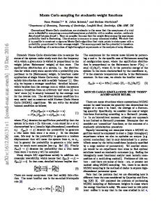
Figure 1: Profiles for Sc representing changing cell populations in each stage with time. (a) had maximal overlap
1
1
0.8
0.8
0.8
0.6
0.4
0.2
0
Cell Fractions
1
Cell Fractions
Cell Fractions
with G2/M genes, (b) with M and M/G1 genes, (c) with M/G1 genes, (d) with G1 and S genes, (e) with S genes
0.6
0.4
0.2
2
4
6
8 10 12 Timepoints
14
16
18
0
0.4
0.2
2
4
6
8 10 12 Timepoints
(a)
14
16
18
0
2
4
6
(b) 1
1
0.8
0.8
Cell Fractions
Cell Fractions
0.6
0.6
0.4
0.2
0
8 10 12 Timepoints
14
16
18
(c)
0.6
0.4
0.2
2
4
6
8 10 12 Timepoints
(d)
14
16
18
0
2
4
6
8 10 12 Timepoints
14
16
18
(e)
Figure 2: Profiles for Sa representing changing cell populations with time. (a) had maximal overlap with G1 genes, (b) with S genes, (c) with M and G2/M genes, (d) with α-factor genes and early G1 genes, (e) with M/G1 genes
1
0.8
0.8
0.8
0.6
0.4
0.2
0
Cell Fractions
1
Cell Fractions
Cell Fractions
1
0.6
0.4
0.2
2
4
6 8 Timepoints
10
0
12
2
4
6 8 Timepoints
10
12
0
2
4
6 8 Timepoints
(b)
1
1
0.8
0.8
Cell Fractions
Cell Fractions
0.4
0.2
(a)
0.6
0.4
0.2
0
0.6
10
12
(c)
0.6
0.4
0.2
2
4
6 8 Timepoints
(d)
10
12
0
2
4
6 8 Timepoints
10
12
(e)
Figure 3: Profiles for La representing changing cell populations with time. (a) had maximal overlap with α-factor genes and early G1 genes, (b) with M/G1 and G1 genes, (c) with S genes, (d) with G2/M, M and M/G1 genes. (e) had genes involved in cell growth and maintenance
direction is to find mathematical justifications for the modifications proposed in Section 2.7 and develop more sophisticated methods to resolve this problem. Finally our approach assumes that gene expressions at a timepoint are independent of each other given a biological stage. We hope to extend our model to incorporate dependencies between gene expressions.
6
Acknowledgments
We would like to thank Dr. Linda Breeden and Dr. Pramila Tata for making their dataset available to us and Dr. Peter Wentzell for helpful discussions. This work was supported by grants from the NSF (MCB0092364) and NIH (HG02262).
References [1] S. Arulampalam, S. Maskell, N. Gordon, and T. Clapp. A tutorial on particle filters for on-line nonlinear/non-gaussian bayesian tracking. IEEE Transactions on Signal Processing, 2002. [2] L. L. Breeden. Cyclin transcription: Timing is everything. Current Biology, 2000. [3] S. Cooper and K. Shedden. Microarray analysis of gene expression during the cell cycle. Cell and Chromosome, 2003. [4] A. P. Dempster, N. M. Laird, and D. B. Rubin. Maximum likelihood from incomplete data via the em algorithm. Journal of the Royal Statistical Society, 1977. [5] A. Doucet, S. Godsill, and C. Andrieu. On sequential monte carlo sampling methods for bayesian filtering, 1998. [6] N. Friedman, M. Linial, I. Nachman, and D. Pe’er. Using bayesian networks to analyze expression data. In RECOMB, pages 127–135, 2000. [7] B. Futcher. Cell cycle synchronization. Methods in Cell Science, 1999. [8] N. Gordon, D. Salmond, and A. Smith. Novel approach to nonlinear /nongaussian bayesian state estimation. IEE Proceedings-F (Radar and Signal Processing), 1993. [9] GO term finder. http://db.yeastgenome.org/cgi-bin/go/gotermfinder. [10] Gene Ontology. http://www.geneontology.org. [11] T. Hastie, R. Tibshirani, and J. Friedman. The Elements of Statistical Learning: Data Mining, Inference, and Prediction. Springer, 2001. [12] M. Isard and A. Blake. Condensation – conditional density propagation for visual tracking. Internation Journal of Computer Vision, 1998. [13] P. Lu, A. Nakorchevskiy, and E. M. Marcotte. Expression deconvolution: A reinterpretation of DNA microarray data reveals dynamic changes in cell populations. Proceedings of the National Academy of Sciences of the United States of America, 2003. [14] V. L. Mackay, B. Mai, L. Waters, and L. L. Breeden. Early cell cycle box-mediated transcription of CLN3 and SWI4 contributes to the proper timing of the G1-to-S transition in budding yeast. Molecular and Cellular Biology, 2001. [15] B. Mai, S. Miles, and L. L. Breeden. Characterization of the ECB binding complex responsible for the M/G1-specific transcription of CLN3 and SWI4. Molecular and Cellular Biology, 2002. [16] T. Minka. Estimating a dirichlet distribution. Technical report, MIT, 2003. [17] A. Niemist¨ o, T. Aho, H. Thesleff, M. Tiainen, K. Marjanen, M. Linne, and O. Yli-Harja. Estimation of population effects in synchronized budding yeast experiments. In Image Processing: Algorithms and Systems II, 2003. [18] A. Niemist¨ o, M. Nykter, T. Aho, H. Jalovaara, K. Marjanen, M. Ahdesm¨ aki, P. Ruusuvuori, M. Tiainen, M. Linne, and O. Yli-Harja. Distribution estimation of synchronized budding yeast population. In Winter International Symposium on Information and Communication Technologies, 2004.
[19] L. R. Rabiner. A tutorial on hidden markov models and selected applications in speech recognition. IEEE, 1989. [20] L. R. Rabiner and B. H. Juang. An introduction to hidden Markov models. IEEE ASSP Magazine, 1986. [21] P. T. Spellman, G. Sherlock, M. Q. Zhang, V. R. Iyer, K. Andres, M. B. Eisen, P. O. Brown, D. Botstein, and B. Futcher. Comprehensive identification of cell cycle-regulated genes of the yeast saccharomyces cerevisiae by microarray hybridization. Molecular Biology of the Cell, 1998.