A Signal Processing Approach to Symmetry Detection - CiteSeerX

1

A Signal Processing Approach to Symmetry Detection Y. Keller, Member, IEEE,, Y. Shkolnisky

Abstract— We present an algorithm that detects rotational and reflectional symmetries of two-dimensional objects. Both symmetry types are effectively detected and analyzed using the Angular Correlation (AC), which measures the correlation between images in the angular direction. The AC is accurately computed using the pseudo-polar Fourier transform, which rapidly computes the Fourier transform of an image on a near-polar grid. We prove that the AC of symmetric images is a periodic signal whose frequency is related to the order of the symmetry. This frequency is recovered via spectrum estimation , which is a proven technique in signal processing with a variety of efficient solutions. We also provide a novel approach for finding the center of symmetry, and demonstrate the applicability of our scheme to the analysis of real images.

I. I NTRODUCTION Symmetry detection and analysis is a fundamental task in computer vision. Naturally, most man-made and biological objects exhibit some extent of symmetry. Consider for example man-made objects such as airplanes and houses or nature-made objects like fish and insects. Thus, symmetry is an effective cue for visual recognition. This approach is supported by experimental analysis of perceptual grouping and attention in the human visual system [1]. The two most common types of symmetries are rotational and reflectional. An object is said to have rotational symmetry of order N if it is invariant under rotations of 2π N n, n = 0 . . . N − 1. An object is said to have reflectional symmetry if it is invariant under a reflection transformation about some line. Hence, symmetry (of both kinds) is an angular property, and as images are given on Cartesian grids, the polar nature of the problem poses computational difficulties. The algorithm presented in this paper uses the pseudopolar Fourier transform (PPFT) [2] to analyze the angular properties of images in the Fourier domain. This approach has several advantages. First, a polar FFT is used to generate a polar representation of the image in an algebraically accurate way. Second, by analyzing the magnitude of the polar FFT, we avoid the need to compute the center of rotation, as the magnitude of the FFT is invariant to translations and commutative to rotations. Third, we reformulate the problem of estimating the order of symmetry as the analysis of a periodic one-dimensional signal embedded in noise. This is a well-known problem in signal processing with well-tested algorithmic solutions. The paper is organized as follows. Section II presents previous works related to symmetry detection. Section III provides a mathematical presentation of symmetries as well This work was supported by a grant from the Ministry of Science, Israel.

as the angular properties of the Fourier domain. Section IV presents the Angular Correlation (AC) as a tool for analyzing symmetries, while discretization and implementation issues are discussed in Section V. Finally, Sections VI and VII present experimental results and concluding remarks, respectively. II. P REVIOUS WORK Symmetry is thoroughly studied in the literature from theoretical, algorithmic, and applicative perspectives. Theoretical treatment of symmetry can be found in [9], [17]. The algorithmic approaches to symmetry detection can be divided into several categories based on their characteristics. The first characteristic of a symmetry detection algorithm is whether it considers symmetry as a binary or continuous feature, which measures the amount of symmetry. A second characteristic is the type of symmetry detected by the algorithm. Most algorithms detect either rotational or reflectional symmetry but not both. A third characteristic is the assumptions that are made on the image. For example, whether the algorithm assumes that the image is symmetric or detects it, or whether the algorithm assumes that the symmetry center is located at the center of the image. A fourth characteristic is whether the algorithm operates in the image domain or transforms the problem into a different domain, such as the Fourier domain. A fifth characteristic is the robustness of the algorithm to noise and its ability to operate on real-life non-synthetic images. We start by describing local symmetry measures. A lowlevel, context free operator for detecting points of interest within an image, which relies on the assumption that context free attention is directed by symmetry, is presented in [13]. The suggested symmetry operator constructs the symmetry map of the image by assigning a symmetry magnitude and symmetry orientation to each pixel. This map is an edge map where the magnitude and orientation of each edge depend on the symmetry associated with each of its pixels. The proposed operator allows one to process different symmetry scales, enabling it to be used in multi-resolution schemes. The proposed operator is demonstrated to be effective in detecting points of interest in natural images. An algorithm for detecting areas with high local reflectional symmetry that is based on a local symmetry operator is presented in [6]. It defines a 2D reflectional symmetry measure as a function of four parameters x, y, θ, and r, where x and y are the center of the examined area, r is its radius, and θ is the angle of the reflection axis. Examining all possible values of x, y, r, and θ is computationally prohibitive; therefore, the algorithm formulates the problem as a global optimization

2

problem and uses a probabilistic genetic algorithm to find the optimal solution efficiently. As noted previously, symmetry can be considered either as a binary or as a continuous feature. A symmetry distance, which measures the amount of symmetry in an object, is presented in [18]. For an object, given by a sequence of points, the symmetry distance is defined as the minimum distance in which we need to move the points of the original object in order to obtain a symmetric object. This also defines the symmetry transform of an object as the symmetric object that is closest to the given one. Algorithms that compute the symmetry transform of an object with respect to rotational and reflectional symmetries, and handle the problem of selecting points to represent 2D objects are described in [18]. These algorithms require finding point correspondences, which is generally difficult, and perform an exhaustive search over all potential symmetry axes, which is computationally expensive. Pattern analysis approaches to symmetry detection define a pixelwise feature vector, which encodes the geometrical structure around each pixel and acts as a local symmetry measure. Then, pixels with similar symmetry measures are clustered together. Such a scheme that detects local, global, and skewed symmetries is described by [15], where an affine invariant feature vector is computed over a set of interest points. Another pattern analysis approach is introduced in [11], where the feature vector field is based on the location, orientation, and magnitude of the edge gradients. Local features in the form of Taylor coefficients of the field are computed and a hashing algorithm is then applied to detect pairs of points with symmetric fields. A voting scheme is used to robustly identify the location of the symmetry axes. The works in [4] and [8] are of particular relevance to our approach, as these schemes operate in the Fourier domain, are able to efficiently detect large symmetric objects, and are considered state of the art. [4] analyzes the symmetries of real objects by computing the Analytic Fourier-Mellin transform (AFMT). The input image is interpolated on a polar grid in the spatial domain before computing the FFT, resulting in a polar Fourier representation. Yet, this approach comes at the cost of losing the shift invariance of the Fourier magnitudes and thus can only be applied to images with known symmetry centers. [8] provides an elegant approach to analyzing the angular properties of an image, without computing its polar DFT. An angular histogram is computed by detecting and binning the pointwise zero crossings of the difference of the Fourier magnitude in Cartesian coordinates along rays. The histogram’s maximum corresponds to the direction of the zero crossing. For real images, most of the zero-crossings detected in the Fourier domain are spurious and the binning operation might result in erroneous maximum. Our approach differs from the above-mentioned schemes in two attributes. First, it uses the pseudo-polar Fourier transform to compute an accurate, translation-invariant polar Fourier representation of the input image. Second, it uses the MUSIC [10] scheme to robustly estimate the order of symmetry. Using the polar representation we define the Angular Correlation (AC), which measures the correlation between images in

the angular direction. We rigorously show that the AC of a symmetric image is a periodic signal whose number of periods corresponds to the order of symmetry. For real images, even the AC computed by our scheme (which is algebraically accurate) is noisy, due to non-perfect symmetries and the nonsymmetric backgrounds (note the Pentagon example in Section V). Hence, we employ a robust, state-of-the-art spectrum estimation technique that enables to analyze real images without preprocessing. Our scheme can also be used to detect multiple symmetric objects within the analyzed image (similarly to local methods [6], [5], [15]), by dividing the input image to sub-images and processing each of them separately. In terms of pattern analysis, our scheme assumes the existence of a global periodic pattern which is best detected by spectral methods (spectrum estimation). This occurs in images containing large symmetric objects, where we are able to robustly identify high order symmetries. In contrast, local pattern analysis schemes [11], [15] are better at detecting cluttered, small symmetric objects, which do not correspond to global periodic patterns. III. M ATHEMATICAL PRELIMINARIES A. Types of symmetries Definition 3.1 (Rotational symmetry): A function ψ : R2 → R is rotationally symmetric of order N around the origin if ψ(x, y) = ψ(Rβn (x, y)), (1) 2 2 where βn = 2π N n, n = 0, . . . , N − 1, and Rβn : R → R is a rotation transformation given by ¶ ¶µ µ x cos βn − sin βn . (2) Rβn (x, y) = y sin βn cos βn In operator notation Eq. 1 is written as ψ = ψ ◦ Rβn , while in polar coordinates it is given by

ψ(r, θ) = ψ(r, θ + βn ),

(3)

where βn = 2π N n, n = 0, . . . , N − 1. Definition 3.2 (Reflectional symmetry): A function ψ : R2 → R is reflectionally symmetric with respect to the vector (cos α0 , sin α0 ) if ψ(x, y) = ψ(Sα0 (x, y)), where

µ Sα0 (x, y) =

cos 2α0 sin 2α0

sin 2α0 − cos 2α0

(4) ¶µ

x y

¶ .

(5)

α0 is the tilt angle of the reflection axis of ψ. An image ψ has reflectional symmetry of order N if there are N angles αn that satisfy Eq. 4. In polar coordinates Eq. 4 is written as ψ(r, α0 + θ) = ψ(r, α0 − θ),

(6)

where α0 is the angle of the reflection axis. If an image ψ has rotational symmetry of order N , then it either has reflectional symmetry of order N or has no reflectional symmetry at all

3

[14], [17]. If an image has both rotational and reflectional symmetry then the axes of reflectional symmetry are given by 1 αn = α0 + βn , n = 0, . . . , N − 1, (7) 2 where α0 is the angle of one of the reflection axes, and βn are the angles of rotational symmetry. A function ψ is rotationally symmetric with center (x0 , y0 ), if ψ(x − x0 , y − y0 ) is rotationally symmetric around the origin. Similarly, ψ is reflectionally symmetric with respect to a vector (cos α0 , sin α0 ) that passes through (x0 , y0 ) if ψ(x − x0 , y − y0 ) is reflectionally symmetric with respect to the vector (cos α0 , sin α0 ) as given by Definition 3.2. B. Properties of the Fourier transform The Fourier transform is the main tool in deriving and analyzing the proposed scheme. In this section we present the definition of the Fourier transform as well as some of its properties that are required for the derivation of the algorithm. Let f : R2 → C be a function whose modulus is square integrable on R2 . The 2D Fourier transform of f , denoted fˆ(ωx , ωy ) or F(f )(ωx , ωy ), is given by ZZ ∞ fˆ(ωx , ωy ) = f (x, y)e−i(xωx +yωy ) dx dy, (8) −∞

where ωx , ωy ∈ R. The following lemmas are well-known and stated without proofs. Lemma 3.3: If ψ is rotationally symmetric around the origin with order N , then, ψˆ is also rotationally symmetric around the origin with the same order. Explicitly, F(ψ) = F(ψ) ◦ Rβn , n = 0, . . . , N − 1. (9) Lemma 3.4: If ψ is reflectionally symmetric with respect to the vector (cos α0 , sin α0 ), then, ψˆ is also reflectionally symmetric with respect to the same vector. Explicitly, F(ψ) = F(ψ) ◦ Sα0 .

(10)

C. Pseudo-polar Fourier transform Given an image I of size N × N , its 2D Fourier transform, b x , ωy ), is given by denoted as I(ω N/2−1

b x , ωy ) = I(ω

X

I(u, v)e−i(uωx +vωy ) , ωx , ωy ∈ R.

u,v=−N/2

(11) We assume for simplicity that the image I has equal dimensions in the x and y directions and that N is even. If ωx and ωy are sampled on the Cartesian grid (ωx , ωy ) = 2π M (k, l), k, l = −M/2, . . . , M/2 − 1, M = 2N + 1, then, Eq. 11 has the form N/2−1 ∆ b l) = I(k,

X

2πi

I(u, v)e− M

(uk+vl)

,

(12)

u,v=−N/2 M −M 2 ,..., 2

k, l = − 1, which is usually referred to as the 2D DFT of the image I. The parameter M (M > N ) sets the frequency resolution of the DFT. It is well-known that the

DFT of I, given by Eq. 12, can be computed with algorithms having complexity O(M 2 log M ). For some applications it is desirable to compute the Fourier transform of I on a polar grid. Formally, we want to sample the Fourier transform in Eq. 11 on the grid ωx = rk cos θl , ωy = rk sin θl , 2πk rk = , θl = 2πl/L, M k = 0, . . . , M − 1, l = 0, . . . , L − 1,

(13)

for which the Fourier transform in Eq. 11 has the form ∆ b Ibpolar (k, l) = I(r k cos θl , rk sin θl ).

(14)

The grid given by Eq. 13 is equally spaced both in the radial and angular directions 2π , (15) M 2π ∆ ∆θp (l) = θl+1 − θl = . (16) L The pseudo-polar Fourier transform defined below produces b It is accurate and can be non-uniform polar samples of I. computed using a fast algorithm. Thus, for practical implementations, we use the pseudo-polar grid instead of the polar one. The pseudo-polar Fourier transform (PPFT) evaluates the 2D Fourier transform of an image on the pseudo-polar grid, which approximates the polar grid. Formally, the pseudo-polar grid is given by the set of samples ∆

∆rp (k) = rk+1 − rk =

∆

P = P1 ∪ P2

(17)

where 2π 2l N N (− k, k) | − ≤ l ≤ , −N ≤ k ≤ N } M N 2 2 (18) 2l N N ∆ 2π P2 = { (k, − k) | − ≤ l ≤ , −N ≤ k ≤ N }. M N 2 2 (19) ∆

P1 = {

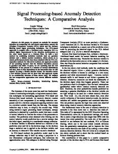
The pseudo-polar grid P is illustrated in Fig. 1c. As can be seen from Figs. 1a and 1b, k serves as a “pseudo-radius” and l serves as a “pseudo-angle”. The resolution of the pseudo-polar grid is N + 1 in the angular direction and M = 2N + 1 in the radial direction. Using a polar coordinate representation, the pseudo-polar grid is given by P1 (k, l) = (rk1 , θl1 ),

P2 (k, l) = (rk2 , θl2 ), s µ ¶ 2 2πk l 1 2 + 1, rk = rk = 4 M N µ ¶ µ ¶ 2l 2l 1 2 θl = π/2 − arctan , θl = arctan , N N

(20) (21)

(22)

where k = −N, . . . , N and l = −N/2, . . . , N/2. We define the pseudo-polar Fourier transform as the samples of the b given in Eq. 11, on the pseudo-polar Fourier transform I, grid P , given by Eq. 17. Formally, the pseudo-polar Fourier

4

(b) The pseudopolar sector P2

(c) The pseudopolar grid.

Fig. 1. The pseudo-polar grid. (a) and (b) are the pseudo-polar sectors P1 and P2 , respectively. (c) The pseudo-polar grid P = P1 ∪ P2 .

transform IbPj P (j = 1, 2) is a linear transformation, which is defined for k = −N, . . . , N and l = −N/2, . . . , N/2, as 2l ∆ b 2π IbP1 P (k, l) = I( (− k, k)), M N 2l ∆ b 2π (k, − k)), IbP2 P (k, l) = I( M N

(23) (24)

where Ib is given by Eq. 11. As we can see in Fig. 1c, for each fixed angle l, the samples of the pseudo-polar grid are equally spaced in the radial direction. However, this spacing is different for different angles. Also, the grid is not equally spaced in the angular direction, but has equally spaced slopes. Formally, 2 ∆ 1 1 ∆ tan θpp (l) = cot θl+1 − cot θl1 = , (25) N 2 ∆ 2 2 − tan θl2 = , (l) = tan θl+1 ∆ tan θpp (26) N where θl1 and θl2 are given in Eq. 22. Two important properties of the pseudo-polar Fourier transform are that it is invertible and that both the forward and inverse pseudo-polar Fourier transforms can be implemented using fast algorithms. Moreover, their implementations require only the application of 1D equispaced FFTs. In particular, the algorithms do not require re-gridding or interpolation. The algorithm for computing the pseudo-polar Fourier transform is based on the fractional Fourier transform (FRFT). The fractional Fourier transform [16], with its generalization given by the Chirp Z-transform [12], is a fast O(N log N ) algorithm that evaluates the Fourier transform of a sequence X on any set of N equally spaced points on the unit circle. By using the fractional Fourier transform we compute the pseudo-polar Fourier transform IbP1 P , given in Eq. 23, as follows Algorithm 1 Computing the pseudo-polar Fourier transform 1: Zero pad the image I to size N × (2N + 1) (along the y direction). 2: Apply the 1D Fourier transform to each column of I (along the y direction). 3: Apply the fractional Fourier transform to each row (in the x direction) with α = 2k/n, where k is the index of the row. The algorithm that computes IbP2 P is similar. The complexity of computing IbP1 P of an N × N image is O(N 2 log N ). Since the complexity of computing IbP2 P is also O(N 2 log N ), the total complexity of computing the pseudo-polar Fourier transform is O(N 2 log N ).

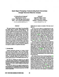
Definition 4.1: Let ψ : R2 → R. The Angular Correlation (AC), denoted gψ (θ), of ψ(r, θ) and ψ(r, −θ) is given by hψ(r, θ)ψ(r, −θ)i − hψ(r, θ)i hψ(r, −θ)i . (29) σ(ψ(r, θ)) σ(ψ(r, −θ)) ¿From the definition, −1 ≤ gψ (θ) ≤ 1. It is clear that if ψ is rotationally symmetric of order N (Definition 3.1), then hψi and σ(ψ) are periodic with N periods over [0, 2π). An example of the AC of a symmetric image is given in Fig. 2. gψ (θ) =

1 0.8 0.6 0.4

gψ(θ)

(a) The pseudopolar sector P1

IV. C ONTINUOUS FORMULATION A. Computing the order of symmetry of centered symmetries For a function ψ : R2 → R, given in polar coordinates, we define its expectation with respect to r over the interval [0, r0 ] as Z dr 1 r0 hψi = ψ(r, θ) . r0 0 r Due to numerical problems arising in its computation, according to [3], we use the following expression Z 1 r0 ν dr r ψ(r, θ) hψi = (27) r0 0 r with ν = 1. We define the standard deviation of ψ with respect to r as q 2 σ(ψ) = hψ 2 i − hψi . (28)

0.2 0 −0.2 −0.4 −0.6 −0.8 −1

0

(a)

θ

π

(b)

Fig. 2. The Angular Correlation function gψ (θ) of a symmetric image. gψ (θ) contains three periods corresponding to the order of rotational symmetry in (a).

Lemma 4.2: If ψ is rotationally symmetric of order N , as given by Definition 3.1, then gψ (θ), given by Eq. 29, is periodic with period β1 = 2π/N . Moreover, gψ (βn ) = 1, n = 0, . . . , N − 1. Proof: From Eq. 3 and the fact that βn = 2π N n we get for n = 0, . . . , N − 1 hψ(r, θ + βn )ψ(r, −(θ + βn ))i gψ (θ + βn ) = σ(ψ(r, θ + βn ))σ(ψ(r, −(θ + βn ))) hψ(r, θ + βn )i hψ(r, −(θ + βn ))i − σ(ψ(r, θ + βn ))σ(ψ(r, −(θ + βn ))) hψ(r, θ)ψ(r, −θ)i − hψ(r, θ)i hψ(r, −θ)i = σ(ψ(r, θ))σ(ψ(r, −θ)) = gψ (θ). Since gψ (0) = 1 and gψ (θ) is periodic, it is clear that gψ (βn ) = 1, n = 0, . . . , N − 1. Lemma 4.2 suggests that it is possible to compute the order of symmetry of ψ by finding the number of periods of gψ (θ) in [0, 2π]. The symmetry axes for reflectional symmetry are then given by 1 αn = α0 + βn , n = 0, . . . , N − 1, 2 where α0 is the tilt angle of one of the axes.

5

B. Finding the tilt angle of a reflection axis The following lemma shows how to compute α0 by relating it to the registration of two images Lemma 4.3: The tilt angle of one of the reflection axes of an image ψ(r, θ), denoted α0 , can be computed by registering ψ(r, θ) to ψ(r, −θ). Proof: By Eq. 6 we have ψ(r, −θ) = ψ(r, α0 + (−θ − α0 )) = ψ(r, α0 − (−θ − α0 )) = ψ(r, 2α0 + θ). Hence, ψ(r, θ) and ψ(r, −θ) are related by a rotation angle of 2α0 . Lemma 4.3 is exemplified by Fig. 3. Next, we show that rotated images can be registered by a variant of the Angular Correlation given in Definition 4.1. Lemma 4.4: Let ψ1 : R2 → R, ψ2 : R2 → R, and define gψ1 ,ψ2 (θ) = hψ1 (r, θ)ψ2 (r, −θ)i − hψ1 (r, θ)i hψ2 (r, −θ)i . σ(ψ1 (r, θ)) σ(ψ2 (r, −θ))

(30)

If ψ2 is a rotated replica of ψ1 , that is ψ2 (r, θ) = ψ1 (r, θ + ∆θ), then gψ1 ,ψ2 (∆θ/2) = 1. Proof: Since ψ2 (r, θ) = ψ1 (r, θ + ∆θ), we have that ψ2 (r, −θ) = ψ1 (r, −θ + ∆θ). Substituting into Eq. 30 we get gψ1 ,ψ2 (θ) = hψ1 (r, θ)ψ1 (r, −θ + ∆θ)i − hψ1 (r, θ)i hψ1 (r, −θ + ∆θ)i , σ(ψ1 (r, θ)) σ(ψ1 (r, −θ + ∆θ)) (31) and gψ1 ,ψ2 (∆θ/2) = 1. Next, we apply Lemma 4.4 to the particular problem of recovering the symmetry axis’ angle. Theorem 4.5: Given a reflectionally symmetric image ψ(r, θ), the angle of its reflection axis, denoted α0 , can be estimated from gψ1 ,ψ2 (θ) with ψ1 (r, θ) = ψ(r, θ) and ψ2 (r, θ) = ψ(r, −θ). In this case, gψ1 ,ψ2 (θ) is denoted as gψ+ ,ψ− (θ). Proof: Let ψ1 (r, θ) = ψ(r, θ) and ψ2 (r, θ) = ψ(r, −θ). Using Lemma 4.3 ψ1 and ψ2 are related by a rotation of 2α0 . This angle is recovered by applying the registration scheme suggested in Lemma 4.4; moreover, gψ+ ,ψ− (α0 ) = 1. The application of Theorem 4.5 to the magnitudes of the Fourier transforms of the images to register allows to recover α0 regardless of the relative translation between the images. Theorem 4.6: The angular correlation between the magnitudes of the Fourier transforms of the images to register shows two maxima over [0, π]. The maxima are π2 apart and can be mapped into the interval [0, π/2]. The implementation requires the rotation of the input images by an arbitrary predefined angle γ. Proof: From¯ the conjugate symmetry of the Fourier ¯ ¯ ¯ ¯b ¯ ¯b ¯ transform we get ¯ψ(r, θ)¯ = ¯ψ(r, θ + π)¯. Hence, the equation g ψb + , ψb − (θ) = 1 (Eq. 31) has at least two solutions. | | | | The first solution is θ0 = ∆θ/2, where ∆θ is the relative rotation between the images. The second, which results from

¯ ¯ ¯ ¯ ¯ˆ ¯ ¯ˆ ¯ the conjugate symmetry ¯ψ(r, θ0 )¯ = ¯ψ(r, −θ0 + ∆θ + π)¯, is θ1 = ∆θ/2+π/2. We combine the two solutions to improve the robustness and accuracy of the estimation by defining π (32) geψ+ ,ψ− (θ) , g ψb + , ψb − (θ) + g ψb + , ψb − (θ + ) | | | | | | | | 2 and computing ½ ¾ θ0 = arg max ge ψb + , ψb − (θ) . | | | | θ∈[0,π/2] For reflectionally symmetric images, ψ(r, α0 + θ) = ψ(r, α0 − θ). Thus, if α0 = 0 and ψ(r, α0 − θ) is computed by flipping ψ upside down then ψ1 (r, θ) = ψ(r, θ) = ψ(r, −θ) = ψ 2 (r, θ) and g ψb + , ψb − (θ) = 1 for every θ. This means that in this | | | | case it is impossible to recover ∆θ from g ψb + , ψb − (θ). Hence, | | | | the image has to be flipped around an axis which is not b θ) to a symmetry axis, and so instead of registering ψ(r, b b b ψ(r, −θ), we register ψ(r, θ) to ψ(r, −θ + γ), where γ is an arbitrary chosen angle. Hence, α0 can be recovered by registering ψ(r, θ) to ψ(r, −θ) using the Angular Correlation, where ψ(r, −θ) is computed by flipping ψ(r, θ) upside down. The robustness is improved by utilizing our knowledge of the order of symmetry N . The registration problem in Theorem 4.5 has N solutions (see Fig. 3), and thus, geψ+ ,ψ− (θ) has N periods over [0, π/2], that is, π geψ+ ,ψ− (α0 ) = geψ+ ,ψ− (α0 + n), n = 0, . . . , N − 1. 2N We denote by geψ+ ,ψ− (α0 ) the reflectional Angular Correlation, as it measures the angular correlation of an image with its reflected replica. Similarly to Eq. 32, we utilize £ π ¤the periodicity by folding geψ+ ,ψ− (θ) from [0, π/2] to 0, 2N geP (θ) =

N −1 X k=0

geψ+ ,ψ− (θ + k

π ), 2N

(33)

and looking for θ0 = arg max {e gP (θ)} . π θ∈[0, 2N ] Due to the conjugate symmetry mentioned above, both θ0 and θ0 + π2 are possible solutions, corresponding to rotations of 2θ0 and 2θ0 + π, respectively. If N is even, either of them can be used, as both α0 and α0 + π2 are valid tilt angles of a symmetry axis. If N is odd, the ambiguity is resolved by rotating the image according to both angles (2θ0 and 2θ0 +π), computing the phase correlation [7], and choosing the one with the highest correlation peak. Finally, by Theorem 4.6 we have 1 that θ0 = ∆θ 2 = 2 (2α0 + γ) and α0 is given by γ α 0 = θ0 − . (34) 2 As any image can be registered to its rotated replica, we get N = 1 both for non-symmetric images and for images with a single reflectional symmetry axis. Thus, we analyze geψ+ ,ψ− (θ) to see whether it has a dominant maximum.

6

−3

7

−3

x 10

6

x 10

6

5

4

4

2

3

2

0

1

0

−2

−1

−2

−3

(a)

(b)

0

0.5

θ

(c)

1

1.5

−4 0

0.1

0.2

θ

0.3

0.4

0.5

(d)

Fig. 3. Recovering the tilt angle of one of the reflection axes. (a) The image has a reflectional symmetry axis tilted by α0 . (b) The image is flipped upside down and the axis is tilted by an angle −α0 . Note that there are three equivalent solutions for the registration of (b) to (a). (c) The reflectional Angular Correlation g eψ+ ,ψ− (θ) computed by (a) and (b). The three maxima corresponding to the three solutions are evident. (d) Folding the three periods gives the basic interval g eP (θ), whose maximum corresponds to the angle α0 .

Consider for example Figs. 5 and 7: in both cases the function gψ (θ) has a single period and the difference being the number of periods, as geψ+ ,ψ− (θ), has no periods in Fig. 7 compared to one in Fig. 5. C. Computing the order of symmetry of non-centered symmetries

itself by rotating ψ by θ = 2π N (N is already known at this point) and recovering the residual translation T . Q is given by Q = T Rθ and as C is mapped to itself QC = C, C is the eigenfunction of Q corresponding to the eigenvalue λ = 1. In practice, Q, T , and Rθ are represented as matrices and C is an eigenvector. This is summarized in Algorithm 2.

Algorithm 2 Computing the center of symmetry In this section we extend the approach suggested in Section 1: Rotate the input image by θ = 2π IV-A to handle non-centered symmetries. By using Lemmas N and denote the rotated e image as ψ. 3.3 and 3.4, and the translation invariance of the Fourier 2: Compute the corresponding rotation matrix Rθ . transform’s magnitude, we obtain Lemma 4.7, which enables e using phase 3: Recover the translation T between ψ and ψ to convert non-centered symmetric functions into functions correlation [7]. that are symmetric around the origin. 4: Compute Q = T Rθ . Lemma 4.7: Let ψ1 be a rotationally symmetric function 5: C is an eigenvector of Q corresponding to the eigenvalue of order N around (x0 , y0 ). Then, |ψˆ1 |2 , where ψˆ1 is the 2D λ = 1. Fourier transform of ψ1 , is rotationally symmetric of order N around the origin. Lemma 4.7 suggests the processing of non-centered symmetries by applying the algorithm from Section IV-A to the V. S CHEME DISCRETIZATION magnitude of the Fourier transform of the input function. This Discretizing the approach suggested in Section IV poses gives the order of symmetry N and the reflection axes αn , several difficulties: n = 0, . . . , N − 1. Therefore, the analog of gψ (θ) (Eq. 29) for 1) The continuous formulation is based on a polar represennon-centered functions is defined as D E D ED E tation of the Fourier transform of the input function. In ˆ θ)|2 |ψ(r, ˆ −θ)|2 − |ψ(r, ˆ θ)|2 |ψ(r, ˆ −θ)|2 |ψ(r, order to use this approach in discrete settings, we need a Eψ (θ) = , fast and accurate way to generate a polar representation ˆ θ)|2 ) σ(|ψ(r, ˆ −θ)|2 ) σ(|ψ(r, of the Fourier transform of a discrete image. (35) 2) The formulation of Eψ (θ) in Eq. 35 uses continuous and the algorithm of Section IV-A is applied to ¯Eψ (θ). ¯ ¯ ¯ definitions of expectation and standard deviation, which As ψ1 is real, ψˆ1 is conjugate symmetric ¯ψˆ1 (r, θ)¯ = ¯ ¯ need to be discretized. ¯ˆ ¯ ¯ψ1 (r, θ + π)¯. Thus, N symmetry axes in |ψˆ1 |2 can result We define a discrete polar representation of the continuous from either N or 2N symmetry axes in ψ1 . This ambiguity is Fourier transform ψˆ as 2π π resolved by rotating ψ1 by both θ1 = 2π n o N and θ2 = 2N = N ˆ cos θ, r sin θ) | (r, θ) ∈ Γ , b = ψ(r and comparing the phase correlation peaks [7]. Note that θ1 Ψ is necessarily a valid solution for the rotation for both N and and choose the grid Γ to be the pseudo-polar grid, for which 2N symmetry axes. we have an efficient numerical scheme. To define a discrete version of Eq. 35, we define the discrete expectation as D. Computing the center of symmetry X b = 1 b θ), After computing the order of symmetry N , we recover the hΨi Ψ(r, (36) N (r) center of symmetry C = (x0 , y0 ). Our approach is based (r,·)∈Γ r