A Small-World Network Model for Distributed Storage of Semantic ...

A Small-World Network Model for Distributed Storage of Semantic Metadata A. Leist

K.A. Hawick

Institute of Information and Mathematical Sciences Massey University Albany, North Shore 102-904, Auckland, New Zealand Email: {a.leist,k.a.hawick}@massey.ac.nz

Abstract The growing uptake of semantic web and grid ideas is raising the importance of optimising distribution algorithms for semantic metadata. While it is not yet clear how real-world metadata distribution patterns ought to evolve, practical experience of social and technical networks suggests that a small-world pattern is desirable and practical. We explore simulated small-world networks of semantic metadata and some graph parameters and metrics. We discuss the implications of inter- and intra-domain path lengths for semantic queries on web and grid structures. Keywords: Small-World, Network, Routing, DHT, P2P, RDF, Semantic Web, Semantic Grid 1

Introduction

The semantic web and grid (Berners-Lee et al. 2001, Shadbolt et al. 2006) are growing in popularity and use and it is interesting to consider how practical storage patterns for semantic metadata might evolve, both practically and optimally. Many sociological networks exhibit small-world properties (Newman 2001, Liljeros et al. 2001) and we anticipate that the global semantic web and grid might do the same. In this paper we explore the implications of a smallworld network structure for the distributed storage of semantic metadata in a web or grid environment that is subject to semantic queries. Not only social networks, but also some large and arguably fault resistant networks found in nature, like the metabolic network of Escherichia coli (Wagner & Fell 2001), possess the characteristics of small-world graphs. If this type of graph is used successfully in nature, then why not investigate its usefulness for largescale, decentralised, distributed computer networks? The small diameters of small-world graphs are certainly an appealing property. Semantic grid and semantic web environments rely on metadata and ontologies to enrich resources, both physical and virtual, with additional information. Unlike in the Web that largely consists of documents for humans to read, the semantic data can provide enough information for software programs or agents to act autonomously. “The Semantic Web is a Web of actionable information—information derived from data through a semantic theory” (Shadbolt et al. 2006). A system that is capable of handling large

©

Copyright 2009, Australian Computer Society, Inc. This paper appeared at the 7th Australasian Symposium on Grid Computing and e-Research (AUSGRID 2009), Wellington, New Zealand. Conferences in Research and Practice in Information Technology (CRPIT), Vol. 99, Wayne Kelly and Paul Roe, Ed. Reproduction for academic, not-for profit purposes permitted provided this text is included.

amounts of metadata is necessary to store this information. We propose a small-world network model that scales well with increasing size and show how it can be utilised as a distributed storage system for RDF metadata. A number of frameworks are available for simulating behaviour and performance of grid systems (Hawick & James 2006, Buyya & Murshed 2002), but since we are interested in a highly specific set of network properties, that are computationally expensive to calculate, we have developed the simulations described in this paper as separate programs and algorithms, that might in principle be incorporated into a self-simulating and self-adjusting semantic grid infrastructure. We describe the key ideas of small-world networks in section 2 and the implications for small-world routing in section 3. In section 4 we discuss the underpinning ideas of RDF triples and their importance in considering distributed semantic metada storage networks. We present a description of our model in section 5 and some selected network properties in 6. We offer suggested areas for future work in section 7 and a conclusion in 8. 2

Small-World Networks

“Given any two people in the world, person X and person Z, how many intermediate acquaintance links are needed before X and Z are connected?” (Milgram 1967) This question provoked the social psychologist Stanley Milgram to perform his famous small-world experiment, which has attracted much attention in the literature during the last decade. Not only various social networks (Newman 2001, Liljeros et al. 2001), but also networks found in nature (Jeong et al. 2000, Fell & Wagner 2000, Wagner & Fell 2001) have been found to possess small-world characteristics. Networks are said to show the small-world effect if the mean geodesic distance (i.e. the shortest path between any two vertices) scales logarithmically or slower with the network size for fixed degree k (Newman 2003). They are highly clustered, like a regular graph, yet with small characteristic path length, like a random graph (Watts & Strogatz 1998). The small diameter of these graphs also makes them interesting for large-scale, distributed computer networks (e.g. peer-to-peer networks). The routing algorithms used in such networks attempt to minimise the number of hops needed to send a message from one node to any other node in the network, while making the networks robust against random failures or deliberate attacks. At the same time they attempt to keep the number of neighbours (i.e. the degree) of each node small to reduce the synchronisation overhead of the network. One of the main challenges in the design of a distributed system with small-world characteristics is the discovery of a short path from

the source node of a message to its destination node with only limited knowledge of the network structure. 3

Routing in a Small-World Network

It is impossible to perform a deliberate search in a uniformly random small-world network—that is, a search without the use of expensive broadcasts—because it is impossible to determine the next step in the chain to the destination. This means that a structure of distance needs to exist to forward a message to someone closer to the target (Watts 2003). There are several ways to implement a structure of distance in a computer network. For instance, an n-dimensional lattice could be used, with each edge that has to be traversed to get to a destination vertex being one hop, possibly with a cost attached to each edge that varies from edge to edge. However, with consideration to the requirement to be able to use the system to store semantic metadata, another solution that already provides a solid implementation for both the structure of distance and the metadata storage was selected. The structure of distance is provided by a Distributed Hash Table (DHT) and the storage of semantic metadata is provided through an additional layer to this DHT called Atlas (Atlas Project 2008). Atlas is a distributed storage and querying system for semantic data, more specifically, Resource Description Framework (RDF) (W3C 2004a) and RDF Schema (RDFS) (W3C 2004b) metadata. The development of Atlas started in the context of the European FP6 project OntoGrid. It provides the functionality to store RDF(S) triples in the DHT and to execute queries using the RDF Query Language (RQL). It is implemented on top of the open source DHT Bamboo (Bamboo Project 2008). 4

The Distributed Storage of RDF Triples

Atlas uses the Query Chain (QC) algorithm proposed in (Liarou et al. 2006) to store RDF triples in the DHT and to perform queries over these triples. It stores each triple on three nodes of the DHT. The keys are generated by hashing the subject, predicate, and object of a triple. The value identified by these keys is always the whole triple. This enables the algorithm to perform queries with placeholders for one or two of the triple parts. 4.1

Domains in the Storage Algorithm

The implementation of our prototype extends the QC algorithm with the concept of multiple domains to take advantage of the domains in the implementation of the underlying network model (see section 5). The system needs to know in which domain it should store a given triple or look for the results when performing a query. The goal is to put triples that are related— and thus likely to be part of the same query—into the same domain, thereby reducing the distance between these triples in the identifier namespace of the DHT. The current implementation assumes that triples that have a subject of the same type, that is, the resources used as the subjects of the triples are instances of the same RDFS class, are related. To apply this concept, the system first determines the types (RDF allows a resource to be an instance of multiple classes) of each subject. In most cases a resource is an instance of exactly one class. If, however, the resource is an instance of more than one class, then any one of its types is selected. The use of non-typed nodes is discouraged. Nevertheless, the system also provides a solution for this case, which will be described later. For now we assume that one

class has been found and selected for a given subject node. The domain identifier is generated from the class URI. The prototype expects the class URI to be an http address and uses the concatenated protocol and domain parts as domain identifier. This means that the system assumes that related concepts are defined under the same domain name and, therefore, should end up in the same network domain. For example, the domain identifier http://example.com would be extracted from the class URI http://example.com/ terms/Person. If unrelated concepts are to be defined under the same domain name, then this can be done by either using sub-domains or by modifying the generator of the domain identifiers to include parts of the directory path. If the subject is an instance of more than one class, then the network domain for each of the other classes is determined as well. For each class C with a distinct domain identifier, a triple is generated with the purpose to declare that the respective class is used in domain D of the previously selected type. This reference triple has the following form: C D Each of these reference triples is stored in the domain of its class C. The same is done for all subjects and predicates if the domain identifier extracted from their respective URIs differs from that of the previously selected class. These reference triples are necessary in order to be able to evaluate query path expressions that do not specify the type of the subject at all, or that specify a type but the system does not know if that is the class that was used to determine the domain identifier or not. As mentioned before, the system also provides a solution for the storage of triples with non-typed subjects. In this case, the domain is extracted from the URI of the predicates of triples with the same subject. If one domain identifier is extracted more often than any other, then that one is used. Otherwise, any one of the most often used domain identifiers is selected. If the domain identifier of the subject or of one of the other predicates differs from the selected domain identifier, then a reference triple is added just like when using a class to determine the domain identifier. The reason for using the predicate over the subject URI is that a subject could be a blank node in the RDF graph (W3C 2004c). 4.2

Storing an Example RDF Document

Assume that a user wants to store his contact details in the DHT. To do this, he first has to create an RDF document with the details that he wants to publish: Arno L e i s t

The next step is to invoke the storage system, which parses the RDF/XML file and extracts the triples from it. It then looks for the types of the subject (http://example.com/contact#me) and finds that it is an instance of the class contact:Person. The

target domain (http://www.w3.org) is extracted from the class URI. All triples that were extracted from the RDF/XML document will be stored in this domain: ” Arno ” . ” Leist ” . . .

The system also compares the domain identifiers extracted from the subject and predicate URIs with the target domain and detects that the domain of the subject differs. Thus, the following reference triple is created and stored in domain http://example.com: .

4.3

Executing Queries

A query path expression must contain at least one constant value and may contain one or two variables. If this is given, then the system can determine a domain identifier from one of the constants and use it to look for reference triples that are relevant to the query as well as for intermediate result values for the first query path expression. There is one exception to this rule though: If the only constant in the expression is a literal value, then the user has to explicitly specify the domain identifier. The reason for this limitation is that a literal value can be any string, not necessarily a URI, which is needed to extract the domain identifier. Once a domain is known, the system needs to find out if any relevant reference triples are stored in this domain. To do this, it creates the following lookup query: s e l e c t REFERENCE from ns : usedInDomain {REFERENCE} using namespace ns=&h t t p : / / example . com/ t e r m s /

The placeholder [URI] is replaced with a class, predicate, or subject URI, depending on the available constant. The lookup query expression is prepended to the original query and executed as the first evaluation step. After the lookup query has been performed, the first query path expression of the original query is executed in the current domain and in all domains that are referred to by the results of the lookup query. This procedure is repeated until all query path expressions have been executed. If any matches to the query are found, then these final results are returned to the user. 5

The Model Prototype

Our prototype system is built on top of Atlas and Bamboo. It modifies the implementation to use concepts common to small-world networks for the routing of messages. This mainly affects the Bamboo implementation of the neighbour selection and routing algorithms. One of the additions is the introduction of domains. Every node is a member of exactly one domain that is specified as a parameter when the node is started. The domains represent the clusters that are

characteristic for small-world environments (Newman 2003, Watts 2003). The routing table implementation of the prototype extends and largely replaces the Bamboo routing table. Everything in this implementation revolves around the creation of a small-world environment for the DHT and the routing of messages within and between these small worlds. What it retains is the ring substrate of the DHT, which is formed through a list of the kn (kn = 8 by default) nearest neighbours that is managed by each node ( k2n in either direction). This list is called the node’s leaf set. The routing table implementation differentiates between nodes in the same domain as the local node and nodes in other domains. It literally manages two routing tables, which are accordingly referred to as the near and far routing tables. The advantage of this implementation is that the neighbours can easily be treated in different ways depending on their closeness to the local node. Close, in this case, does not mean that the nodes are located physically near to each other, but close in terms of their identifier in the namespace of the DHT. Since each node only has a limited number of neighbours, messages can only be routed towards the destination node on a best effort basis. This means that a message is first routed as close as possible to the target domain. Thus, the suggested next hop is based on the far routing table of the node that is currently processing the message. If it does not know a node in a domain that is closer to the target than its own domain, then it chooses the closest node to the target from its near routing table. That is, either the node with the lowest or highest identifier is selected. If, on the other hand, the destination node is in the local domain, then it checks the near routing table for the node that is closest to the destination. If none of its neighbours is closer to the target than itself, then the next hop is chosen from the leaf set instead. The leaf set guarantees, assuming that it is consistent and up-to-date, that the message can always be routed further towards the destination node. Both routing tables are split up into segments. The relative number of neighbours in each segment of the domain and global namespaces is called the neighbour distribution. The aspired distribution of neighbours can be configured separately for either of the routing tables. It is specified in form of an integer array of odd length. The array length defines into how many segments the namespace is divided. Each value in the array specifies the relative number of neighbours in that segment. Every node considers itself the center of the distribution. If, for example, the distribution for the near routing table is {1, 2, 3, 2, 1}, then the routing table implementation tries to find x neighbours for the outer segments, 2x neighbours for the segments adjacent to the center segment, and 3x neighbours for the center segment. The number x depends on the size of the routing table. Given that the local node is used as the center of the distribution, one of the segments exceeds the upper or falls below the lower limit of the namespace in almost all cases. Since both the domain and the global namespaces are treated as continuous rings, the segment is wrapped around the upper or lower bound of the respective namespace. The near routing table and even more so the leaf set form the cluster of tightly interconnected friendship relationships common to small-world networks. The far routing table provides the long-distance or “weak” links (Buchanan 2002) that are so important for the transition from a disconnected caveman-world (Watts 1999) to a fully connected small-world network.

6

Network Properties

We have analysed various properties of the network model and present the results in this section. Unless specifically mentioned otherwise, the simulation results illustrated in the charts are averaged over 100 realisations of the network with the same set of parameters. Error bars representing the standard deviation from the mean values are illustrated for all of the results, however, sometimes they are so small that they are completely covered by the symbols. The leaf set size is always kn = 8. The default near routing table size knear = 70 and the default far routing table size kf ar = 30 for a total degree of k = 100. Likewise, the neighbour distribution defaults to {2, 5, 10, 15, 20, 15, 10, 5, 2} for both routing tables. The total number of messages m = N × 50 generated during each realisation of the network depends on the network size N . Each node generates approximately the same number of messages. The destination node for a message is always chosen with similar probability from either all the nodes in the network (1), from the same domain as the source node (2), or from the nodes in the domain of the destination node of the previous message generated with option (2) by the same source node (3). The third method has a slightly lower probability than the first two, because it can not occur until the node has generated at least one message following method (2). The idea behind the third method is to analyse how much the routing tables improve based on previously generated messages. However, the results for method (3) are much more noisy than the results for methods (1) and (2). Thus, they are not particularly meaningful and were omitted in all but one of the charts (see figure 7). This is not very surprising, since the current implementation of the routing table does not take the destination domains of previously sent messages into account when it decides if a node should replace a current neighbour in the routing table. This feature is planned for an improved version of the routing table (see section 7). 6.1

Routing Table Ratios & Distributions

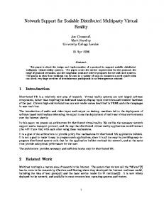
The 70/30 (near/far) ratio for the routing table sizes is based on the simulation results illustrated in figures 1 and 2. Let us consider the default neighbour distribution (circles) for now. The initial assumption was that the near routing table—the cluster of tightly interconnected friends—should be larger than the far routing table—the long-distance links—as described in the literature for small-world environments (Buchanan 2002, Watts 1999). The more the ratio increases in favour of the long-distance links, the more random the network becomes. The results largely support this assumption, showing that the 30/70 ratio yields the highest number of hops needed to deliver the messages. That 70/30 clearly is the best of the analysed ratio settings when sending messages to the same domain as the source node of the message is not surprising, since the far routing table is not used at all in this scenario. Messages sent to a vertex that is randomly chosen from all the vertices in the network slightly benefit from a 50/50 or 60/40 ratio. What is interesting is that even in this case placing more neighbours in the far routing table than in the near routing table does not yield better results. However, these results are likely to be dependent on the number of domains in the network, which was set to 100 for this simulation. Thus, every domain contained approximately 1000 vertices. Figures 3 and 4 illustrate how the number of domains influences the average number of hops needed to deliver a message

Figure 1: The mean number of hops h needed to deliver a message to a destination node for varying near and far routing table size ratios and three different neighbour distributions. The destination nodes are randomly chosen from all nodes in the network. The combined routing table size is always knear + kf ar = k = 100 and the network size is N = 100, 000. The nodes are approximately evenly spread over d = 100 domains and a total of m = 5, 000, 000 messages are generated. The results are averaged over 40 realisations of the network. to a node chosen from all the nodes in the network (1) and to a node chosen from the same domain (2) respectively. The results for (2) are not surprising, the average number of hops decreases with an increasing number of domains (i.e. decreasing domain size). The results for (1) show that the clustering introduced with the domains reduces the path length between nodes as intended. Around 100 domains (i.e. 1000 vertices in each domain) appears to be a good number for the delivery of messages to randomly chosen nodes in a network of N = 100, 000 nodes, independent of the routing table size ratio. But the results also highlight that there can be too many domains, especially when the far routing table is small. The routing table size ratio clearly influences how drastic the results turn out to be. The results for the number of hops illustrated in the charts are the mean values of the group mean values. The first set of mean values is calculated from all messages generated with the same destination node selection method for each of the network realisations. But since always multiple realisations of the network are generated with the same parameter set, the mean values of these group mean values are calculated to gain the final result values. The chart illustrated in figure 5 is an exception and shows the data points for the mean values of 20 result sets for the data of the 70/30 routing table size ratio illustrated in figure 4. The first 20% of the messages were discarded to avoid noise introduced by routing tables that are not completely filled and had no chance to optimise themselves yet. While the mean values are very close together, as also illustrated by the very small standard deviations for the mean values of the group mean values, the deviation from the simple mean values is strong. Individual messages take considerably more or less hops than other messages to reach their destination. Now let us go back to figures 1 and 2 and this time concentrate on the neighbour distributions. The default neighbour distribution for both routing ta-

Figure 2: Like figure 1, only that the destination nodes are randomly chosen from the same domain as the source node. The results are averaged over 40 realisations of the network.

Figure 4: The mean number of hops h needed to deliver a message to a destination node randomly chosen from the same domain as the source node for an increasing number of domains d = 10, . . . , 1010. The network size N = 100, 000 is constant, thus, the number of nodes in each domain decreases with increasing d. 6.2

Clustering Coefficients

The respective clustering coefficients γ for the varying routing table size ratios and neighbour distributions (see figures 1 and 2) are illustrated in figure 6. The clustering coefficient γ of a graph G is γv averaged over all v ∈ V (G). γv is defined as follows (Watts 1999): The clustering coefficient γv of Γv characterises the extend to which vertices adjacent to any vertex v are adjacent to each other. More precisely, γv =

|E(Γv )|
, kv

(1)

2

Figure 3: The mean number of hops h needed to deliver a message to a destination node randomly chosen from all the nodes in the network for an increasing number of domains d = 10, . . . , 1010. The network size N = 100, 000 is constant, thus, the number of nodes in each domain decreases with increasing d. bles {2, 5, 10, 15, 20, 15, 10, 5, 2} is based on these results. The initial assumption was again that an increased cluster formation is beneficial in that it becomes easier to find a short path between nodes than it is in a more random network. The results confirm this assumption for both the messages sent to destination nodes randomly selected from all the nodes in the network and for those selected from the same domain as the source node. While the difference between an even distribution {1} and a distribution centered around the individual nodes {2, 5, 10, 15, 20, 15, 10, 5, 2} is clearly visible, this becomes even more pronounced when comparing to the inverse case {20, 15, 10, 5, 2, 5, 10, 15, 20}, where more neighbours are chosen from the far ends of the namespace as seen from the individual nodes. The results of the latter distribution are also much more noisy than those of the other distributions, showing that the routing algorithm is not optimised for this scenario.

where |E(Γv )| is the number of
edges in the kv neighbourhood of v and 2 is the total number of possible edges in Γv . The results show that the clustering coefficients are rather low for all analysed parameter sets. Surprising is that the results of the clustering metric decrease with increasing near and decreasing far routing table sizes, until a tipping point around 60/40 is reached where the values begin to increase again. It will be interesting to see if this trend continues for values like 80/20. Also unexpected is the intersection of the even {1} and centered {2, 5, 10, 15, 20, 15, 10, 5, 2} distributions. Further simulations will hopefully shed more light on the reasons for this, as we can not yet explain why the even distribution yields a clearly higher clustering than the centered one for routing table ratios that favour the near routing table. 6.3

Scaling

Now that the parameter values for the ratio of the routing table sizes and for the neighbour distributions have been chosen, it can be analysed how well the network scales with increasing network size N . Figure 7 illustrates the results. This chart also includes method (3) of the destination node selection algorithm, showing that the number of hops needed

Figure 5: The individual mean values of 20 result sets for the data of the 70/30 routing table size ratio already illustrated in figure 4. This chart shows the deviation from the mean values of the number of hops needed to deliver messages in individual instances of the network instead of the mean values of the group mean values. The error bars have been rescaled by a factor of 0.1. to deliver a message to a domain that has just recently been the destination of another message generated by the same node is indeed slightly lower than in method (1). However, it also shows the before mentioned strong deviation from the mean values that gets worse the larger the network becomes. Further improvements of the routing table’s neighbour selection algorithms are expected to yield better values for this method. This is done under the assumption that a node tends to send further messages to a domain that has been the target of previous messages than to a random domain (see section 4). What may appear as strange is that all three result sets have roughly the same values for N = 1000. The reason for this is simply that the number of vertices in each domain is fixed to 1000, independent of the network size. Therefore, all nodes are in the same domain and all of the neighbour selection methods choose the destination nodes from all the nodes in the network. As expected, the diagram also shows that the number of hops needed to send a message to a node in the same domain as the source node does not increase with the network size, as long as the number of nodes in each domain is kept constant. What is surprising, however, is that the hop count drops slightly with increasing network size. The reason for this is not yet entirely clear and needs further investigation. A possible explanation is that, even though the number of messages increases linearly with the network size, more messages are routed through the network in total and, thus, the routing tables get more opportunities to learn about other nodes and select the most suitable neighbours. Now that the results for the scaling behaviour of the network are available, they can be used to determine if the goal to create a network that exhibits small-world characteristics has been achieved. The definition given in section 2 says that the shortest path between any two vertices in a small-world graph has to scale logarithmically or slower with the network size for fixed degree k. Due to the computational complexity of the all-pairs shortest path algorithms (see section 7), we are unfortunately not yet able to de-

Figure 6: The clustering coefficients γ for varying near and far routing table size ratios and neighbour distributions. See figure 1 for the network parameters used in this simulation. The results are averaged over 40 realisations of the network. termine this metric for a network with N = 101, 000 and k = 100. But what really counts is not the theoretically shortest number of steps needed to deliver a message, but the number of hops actually needed by the routing algorithms. Figure 8 illustrates the results for method (1) and (2) from figure 7 on a log-log plot. Of particular interest are the results for the scaling of method (1), where the message destination nodes are randomly chosen from all the nodes in the network. They form a straight line on the log-log plot, which highlights that the network actually scales logarithmically with the network size. Therefore, the network behaves like a small-world for values of N that have so far been feasible to evaluate. 7

Discussion & Future Directions

We have presented the simulation results for a number of parameter sets and values. The analysed metrics provide new insights into the effects that different parameters have on the network and into the properties of this network model in general. The computational costs of the simulations unfortunately limit us in the number of parameters and metrics that we can analyse in a given amount of time. However, some additional metrics, like the mean geodesic distance, the number and length of circuits and the network robustness against random failures and deliberate attacks, are worth considering since they might help us better understand and further improve the network model in the future. Additional simulations with different parameter sets are also planned to get more detailed results for some of the metrics described in section 6. For instance, the results illustrated in figure 8 could be extended by plots of the values gained for messages sent to domains in an increasing radius of the source domain. The assumption is that, depending on the neighbour distribution of the far routing table, the results will fill the area between the messages addressed to the same domain and those addressed to a random domain. And while they are expected to also exceed the latter when the radius becomes large enough, it will be interesting to see when exactly this happens. So far the total routing table size has been the same for all realisations of the network (k = 100). This degree has been a mostly arbitrary guess and

Figure 7: The mean number of hops h needed to deliver a message in a network of increasing size N = {1000, 11000, . . . , 101000}. The visible error bars belong to method (3), while the standard deviations for (1) and (2) are so small that they are covered by the symbols. The number of nodes in each domain is fixed to 1000 and, thus, the number of domains d = {1, 11, . . . , 101} increases with the network size. Each node generates on average 50 messages and, therefore, the total number of messages m = {50000, 550000, . . . , 5050000} also increases with the network size. simulations with different degrees may show that a smaller size is sufficient or that a larger size would give considerably better results. In its current incarnation, the routing table takes both the user-defined distribution of neighbours and the latency between nodes into account when it chooses a neighbour. However, the latter has not been incorporated into the network analysis yet. And because the latency is an important property of a distributed network, it would be interesting to see how the network improves in this regard over time. The latency between two neighbours can be modelled as the weight of the arc that represents the neighbourhood relationship. It can then be taken into account when measuring the mean shortest path between any two nodes. Various improvements to the routing table implementation are planned for future versions. These include features like:

ˆ The dynamic assignment of nodes to domains depending on the messages that they generate. If a node sends many messages to a certain domain, then it makes sense to move it into that domain so that it can take advantage of the much lower number of hops needed to deliver messages within the same domain. ˆ An increased probability to add a node to the routing table the more often it is the destination of a message routed through or generated by the local node. ˆ An increase in the clustering behaviour by adding a form of preferential attachment to the neighbour selection algorithm. The preferential attachment could give the “friends of a friend” a higher ranking compared to a random node, making it more likely that they are selected as neighbours. This would effectively increase the number of triangles in the network (Newman 2003). The extent to which this should be done,

Figure 8: The log-log plot of the mean number of hops h needed to deliver a message in a network of increasing size N . See figure 7 for the parameter values. The straight lines are the least square linear fits. The slope of the fit for (1) is ≈ 0.117 and for (2) it is ≈ −0.005. if it prooves to be be beneficial at all, needs to be determined. An important aspect of distributed networks is their robustness against random failures and deliberate attacks. Scale-free networks that consist of very few highly connected hub nodes and many nodes with a low degree are robust against random failure, because it is very unlikely that a hub node fails by random chance. However, they are vulnerable against deliberate attacks, as the hub nodes are the logical target and their failure causes the network diameter to rise sharply, until the network fragments into several isolated clusters. Exponential networks, on the other hand, have no hub nodes that are exceptionally significant for the connectedness of the network. Thus, they do not show a significant difference between random failures and deliberate attacks, but are generally less robust against random failures than scale-free networks (Albert et al. 2000, Buchanan 2002). One of the major problems when analysing large graphs is the computational complexity of some of the algorithms. For example, Dijkstra’s distance algorithm requires O(|V |3 ) time to compute the shortest path between any two vertices in the graph (Gould 1988). However, some of these algorithms can be highly parallelised to be executed on many single instruction multiple data (SIMD) stream processors concurrently. And in this domain the general-purpose computing on graphics processing units (GPGPU) has gained much attention recently. The major graphic card vendors have released software development kits—NVIDIA’s CUDA— Toolkit (NVIDIA® Corporation 2008) and the AMD Stream SDK (Advanced Micro Devices, Inc. 2008)—to support this programming model on their respective GPUs. These have been used to develop new algorithms that yield impressive speed-ups compared to the respective implementations for ordinary CPUs. This also includes algorithms for graph metrics like the before mentioned shortest path problem (Harish & Narayanan 2007). We intend to make use of the capabilities of GPGPU programming in order to be able to analyse larger networks than we currently can within a feasible time frame. This article mainly concentrated on the properties of the underlying network and less on the actual usage

of the network to store and query RDF metadata. Although the implementation has been described in section 4, measurements of its actual performance with realistic data sets have yet to be conducted. 8

Conclusions

We proposed a small-world network model implementation based on a Distributed Hash Table. The network scales well with increasing size, so that even in a large-scale deployment only a few hops are needed to deliver a message between any two nodes. The DHT is divided into clusters or domains. These domains are meant to be used to store related data that is likely to be accessed collectively, taking advantage of the smaller number of hops needed to send messages within the same domain. Furthermore, the cost of delivering a message within a domain grows with the domain size and not with the overall network size, making it even more appealing to separate independent data into different domains. We also showed how this network can be used to store RDF metadata and how this data can be assigned to different domains in order to take advantage of the more efficient delivery of messages within the same domain. This distributed and decentralised storage allows large amounts of metadata, which quickly accumulate in a semantic web or semantic grid environment, to be managed. References

Hawick, K. A. & James, H. A. (2006), Simulating a Computational Grid with Networked Animat Agents, in R. Buyya & T. Ma, eds, ‘ACSW Frontiers ’06: Proceedings of the 2006 Australasian workshops on Grid computing and e-research’, Australian Computer Society, Inc., Darlinghurst, Australia, pp. 63–70. Jeong, H., Tombor, B., Albert, R., Oltvai, Z. & Barabsi, A.-L. (2000), ‘The large-scale organization of metabolic networks’, Nature 407(6804), 651– 654. Liarou, E., Idreos, S. & Koubarakis, M. (2006), Evaluating Conjunctive Triple Pattern Queries over Large Structured Overlay Networks, in ‘Proceedings of the Semantic Web - ISWC 2006: 5th International Semantic Web Conference’, SpringerVerlag, Athens, GA, pp. 399–413. Liljeros, F., Edling, C., Amaral, L., Stanley, H. & Aberg, Y. (2001), ‘The web of human sexual contacts’, Nature 411(6840), 907–908. Milgram, S. (1967), ‘The Small-World Problem’, Psychology Today 1, 61–67. Newman, M. E. J. (2001), ‘The structure of scientific collaboration networks’, PNAS 98(2), 404–409. Newman, M. E. J. (2003), ‘The Structure and Function of Complex Networks’, SIAM Review 45(2), 167–256.

Advanced Micro Devices, Inc. (2008), ‘AMD Stream SDK’, http://ati.amd.com/technology/ streamcomputing/. Last accessed September 2008.

NVIDIA® Corporation (2008), ‘CUDA—: Compute Unified Device Architecture’, http://www. nvidia.com/object/cuda_home.html. Last accessed September 2008.

Albert, R., Jeong, H. & Barabsi, A.-L. (2000), ‘Error and attack tolerance of complex networks’, Nature 406(6794), 378–382.

Shadbolt, N., Hall, W. & Berners-Lee, T. (2006), ‘The Semantic Web Revisited’, IEEE Intelligent Systems 21(3), 96–101.

Atlas Project (2008), ‘Atlas Distributed RDF Metadata Storage and Query System’, http://atlas. di.uoa.gr. Last accessed April 2008.

W3C (2004a), RDF Primer. Last accessed August 2008. URL: http://www.w3.org/TR/rdf-primer/

Bamboo Project (2008), ‘Bamboo Distributed Hash Table’, http://www.bamboo-dht.org. Last accessed April 2008.

W3C (2004b), RDF Vocabulary Description Language 1.0: RDF Schema. Last accessed August 2008. URL: http://www.w3.org/TR/rdf-schema/

Berners-Lee, T., Hendler, J. & Lassila, O. (2001), ‘THE SEMANTIC WEB’, Scientific American 284(5), 34–.

W3C (2004c), Resource Description Framework (RDF): Concepts and Abstract Syntax. Last accessed August 2008. URL: http://www.w3.org/TR/rdf-concepts/

Buchanan, M. (2002), NEXUS - Small Worlds and the Groundbreaking Science of Networks, W.W. Norton & Company. Buyya, R. & Murshed, M. (2002), ‘GridSim: a toolkit for the modeling and simulation of distributed resource management and scheduling for Grid computing’, Concurrency and Computation: Practice and Experience 14(13-15), 1175–1220. Fell, D. A. & Wagner, A. (2000), ‘The small world of metabolism’, Nature Biotechnology 18(11), 1121– 1122. Gould, R. (1988), Graph Theory, The Benjamin / Cummings Publishing Company. Harish, P. & Narayanan, P. (2007), Accelerating large graph algorithms on the GPU using CUDA, in S. Aluru, M. Parashar, R. Badrinath & V. Prasanna, eds, ‘High Performance Computing - HiPC 2007: 14th International Conference, Proceedings’, Vol. 4873, Springer-Verlag, Goa, India, pp. 197–208.

Wagner, A. & Fell, D. A. (2001), ‘The small world inside large metabolic networks’, Proceedings of the Royal Society B 268(1478), 1803–1810. Watts, D. J. (1999), Small Worlds: The Structure of Networks between Order and Randomness, Princeton University Press. Watts, D. J. (2003), Six Degrees - The Science of a Connected Age, W.W. Norton & Company. Watts, D. J. & Strogatz, S. H. (1998), ‘Collective dynamics of ‘small-world’ networks’, Nature 393(6684), 440–442.