A Study of Percolation Phenomena in Process Networks

Communicating Process Architectures 2006 Peter Welch, Jon Kerridge, and Fred Barnes (Eds.) IOS Press, 2006 c 2006 The authors. All rights reserved.

109

A Study of Percolation Phenomena in Process Networks Oliver FAUST, Bernhard H. C. SPUTH and Alastair R. ALLEN Department of Engineering, University of Aberdeen, Aberdeen, AB24 3UE, UK {o.faust , b.sputh , a.allen}@abdn.ac.uk Abstract. Percolation theory provides models for a wide variety of natural phenomena. One of these phenomena is the dielectric breakdown of composite materials. This paper describes how we implemented the percolation model for dielectric breakdown in a massively parallel processing environment. To achieve this we modified the breadth-first search algorithm such that it works in probabilistic process networks. Formal methods were used to reason about this algorithm. Furthermore, this algorithm provides the basis for a JCSP implementation which models dielectric breakdowns in composite materials. The implementation model shows that it is possible to apply formal methods in probabilistic processing environments. Keywords. Percolation, Breadth-first search, JCSP, Probabilistic process networks, channel poisoning

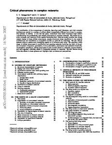
Introduction The percolation problem has been extensively investigated by mathematicians and physicists. In this paper we analyse the problem from a computer science point of view. One of the reasons for this cross disciplinary interest is the fact that the percolation problem yields extremely simple systems exhibiting the intriguing complexities of phase transitions. These systems can be associated with many physical realisations [1,2]. S. R. Broadbent and J. M. Hammersley posed the original percolation problem in the context of graph theory [3]. They considered an arbitrary linear graph, like the one shown in Figure 1, in which the vertices are points of the model, and a given pair of vertices is linked by an edge with probability p independently of all other pairs; this is an example of bond percolation.

Figure 1. A linear graph as one realisation of a bond percolation problem

More recent work has focused on applications of percolation theory in the physical world. Of special interest were connectivity studies in various materials. S. Reder has studied percolation and conduction in a random resistor diode network [4]. Such a network extends the bond percolation theory by allowing directed (diode) and undirected (resistor) edges. Closer to the bond percolation theory are dielectric breakdown models. Such models are used

110

O. Faust, B.H.C. Sputh and A.R. Allen / Percolation Phenomena in Process Networks

to abstract a physical system where conducting particles are distributed at random in an insulating material. A dielectric breakdown between two conducting particles occurs if the distance between them is below a certain threshold. A dielectric breakdown of the insulating material occurs if there is a conducting path through the insulating material. F. Peruani et al. have generalised the dielectric breakdown model (DBM) to describe dielectric breakdown patterns in conductor-loaded composite materials [5]. In this paper we analyse a simple DBM. Figure 2 shows a possible realisation of an experimental dielectric breakdown setup. Each vertex between the two plates represents a conducting particle and an edge indicates that there is an electrical path between the particles. In this particular realisation of the model a dielectric breakdown occurs, because there is a conducting path between the plates. Plate Conducting particle Connecting path

Source

Figure 2. Experimental dielectric breakdown setup

In order to determine whether or not a particular realisation of the experiment is conducting we implemented a simulation setup in a massively parallel processing environment. Each conducting particle is modelled as an individual process. Electrical breakdown between two particles is modelled as a communication channel between two processes. A dielectric breakdown of the material is similar to the ability of the process network to transmit a message from one side to the opposite side over the communication channels between the processes. In general, a message represents a communication between sequential processes. Hoare’s CSP (Communicating Sequential Processes) provides the theoretical basis to reason about such communication in a very skilful manner [6,7]. In this paper we use CSP to derive an elegant solution for the ‘find cluster from node’ problem. The proposed solution does not require any sequentialisation during the algorithm design. With sequentialisation we mean the design of cascaded loops and control structures. Standard solutions for student education and even more sophisticated algorithms, as in [8], use such structures to achieve the required functionality. Unfortunately, the design and implementation of these structures increases complexity and code size of the algorithm. This results in an increased error density [9]. Compared with these sequential algorithms the CSP model yields code with a lower error density, because it is simpler and more compact. To show the practical viability of these ideas we implemented the algorithm using JCSP. The following section provides a short review of percolation theory. Section 2 introduces the find cluster from node algorithm, which is an adaptation of breadth first search for parallel processing platforms. The algorithm is proved for a particular network setup and in a second step it is shown that the algorithm works for an arbitrary network setup. The last section discusses the application of the algorithm in an experimental implementation of a dielectric breakdown model. The model is implemented with JCSP (CSP for Java). Statistical tests show that this implementation behaves according to percolation theory.

O. Faust, B.H.C. Sputh and A.R. Allen / Percolation Phenomena in Process Networks

111

1. Bond Percolation Theory This section briefly establishes the basic definitions and notation of bond percolation in a d dimensional integer space Zd . The main result of this section is the definition of a probability space which allows us to reason about bond percolation problems in terms of probability. From this theoretical discussion we gain sufficient insight to propose the foundations of a practical implementation model. This discussion follows loosely Geoffrey Grimmett’s introduction to percolation [10]. To start we define the (graph-theoretic) distance δ(x, y) from x to y by:

δ(x, y) =

d X

x, y ∈ Zd

| xi − yi |

(1)

i=1

The space Zd is turned into a so called d-dimensional cubic lattice, by adding edges between all pairs x, y of points of Zd with δ(x, y) = 1. We call the resulting lattice Ld and think of Zd as the set of vertices in Ld . The edges are described by Ed . Next we introduce probability to the lattice. Let p and q satisfy 0 6 p 6 1 and q = 1 − p. We declare each edge of Ld to be open with probability p and closed otherwise, independently of all other edges. This can be expressed Q in a more formal way by the following probability space. As sample space we take Ω = e∈Ed {0, 1} points of which are represented as ω = ω(e) : e ∈ Ed and called configurations; the value ω(e) = 0 corresponds to e being closed, and ω(e) = 1 corresponds to e being open. We take F to be the σ-field of subsets of Ω generated by the finite-dimensional cylinders. Finally, we take product measure with density p on (ω, F): Pp =

Y

µe

(2)

e∈Ed

where µe is the Bernoulli measure on {0, 1}, given by µe (ω(e) = 0) = q

µe (ω(e) = 1) = p

(3)

We write Pp for this product measure, and Ee for the corresponding expectation operator. The probability space is summarised as (Ω, F, Pp ). We used the following device to construct the experimental setup described in the subsequent sections. Suppose that (X(e) : e ∈ Ed ) is a family of independent random variables indexed by the edge set Ed , where each X(e) is uniformly distributed in the range [0, 1]. We may couple together all bond percolation processes on Ld as p ranges over the interval [0, 1] in the following way. Let p satisfy 0 6 p 6 1 and define ηp (∈ Ω) as: ( 1 if X(e) < p ηp (e) = 0 if X(e) > p

(4)

We say that the edge e is p-open if ηp (e) = 1. The random vector ηp has the following properties: P(ηp (e) = 0) = 1 − p,

P(ηp (e) = 1) = p

(5)

112

O. Faust, B.H.C. Sputh and A.R. Allen / Percolation Phenomena in Process Networks

We may think of ηp as being the random outcome of the bond percolation process on L with edge-probability p. Now, ηp1 6 ηp2 whenever p1 6 p2 , which is to say that we may couple together two percolation processes with edge probabilities p1 and p2 in such a way that the set of open edges of the first process is a subset of the set of open edges of the second. More generally, as p increases from 0 to 1, the configuration ηp runs through typical configurations of percolation processes with all edge probabilities. Figure 3 shows a realization of bond percolation on a 20 × 20 section of the two dimensional (d = 2) square lattice for p1 = 0.2. This means each edge exists with a 20% chance. In Figures 4 – 6 p is increased by 0.2 for each try, such that p1 = 0.2 < p2 = 0.4 < p3 = 0.6 < p4 = 0.8. The seed for the random variable is the same (seed = 3) for all realisations, therefore the set of edges of the first realisation is a subset of the set of edges of the second and so on, and the 4th realisation contains all edges of the previous realisations. We say that each graph is a subgraph of the next. d

Figure 3. Realisation: 20 × 20, p1 = 0.2, seed = 3

Figure 4. Realisation: 20 × 20, p2 = 0.4, seed = 3

Figure 5. Realisation: 20 × 20, p3 = 0.6, seed = 3

Figure 6. Realisation: 20 × 20, p4 = 0.8, seed = 3

1.1. The Critical Phenomenon In the introduction we stated that the percolation problem yields extremely simple systems exhibiting the intriguing complexities of phase transitions. To discuss phase transitions, it is necessary to define the critical quantity of interest. For percolation problems this is the so called percolation probability θ(p) which is the probability that an infinite cluster exists in the

O. Faust, B.H.C. Sputh and A.R. Allen / Percolation Phenomena in Process Networks

113

graph. Figure 7 indicates how the percolation probability θ(p) depends on the edge existence p. The exact relationship depends on the dimension of the graph d. Harry Kesten proved that the phase transition probability for a two dimensional graph is θc (2) = 0.5 [11]. Section 3 provides a validation of that result. θ(p) (1, 1)

1

p 0

pc (d)

1

Figure 7. Theoretical percolation probability θ(p)

2. Find Cluster from Node Algorithm This section describes an adaptation of the breadth first search algorithm for massively parallel processing systems. The proposed algorithm discovers all nodes which are connected over a path to one particular node, therefore the algorithm is called find cluster from node. In a first step the algorithm discovers the network by spreading over every available channel. If there are no new nodes to discover, each individual node returns its ID and the IDs from all other nodes it received to the node which initially discovered the node under discussion. To investigate the algorithm in further detail, the following subsection provides a CSP model of the algorithm for a particular network. The network, shown in Figure 8, consists of 5 nodes (processes) and directed edges (channels) between them. A connection between two processes is established by connecting them with two channels in opposite directions. The channels are named c.from.to where from represents the sender ID and to is the receiver ID. The process S has the ID 0, it is a special process because it can initiate the find cluster from node algorithm. 2.1. CSP Model As a first step in the CSP model the network setup is defined with a configuration function CFG(x) where x is a process ID. For a specific process ID x, the configuration function returns a set of process IDs. This set defines to which processes the process with ID x is connected. Equation 6 defines the configuration function for the network shown in Figure 8.

CFG(1) ={0, 2, 3} CFG(2) ={1, 3, 4} CFG(3) ={1, 2} CFG(4) ={2}

(6)

The process S initiates the discovery phase of the find cluster from node algorithm by sending an empty set {} to P(1). After that the process S expects the result, i.e. a set with

114

O. Faust, B.H.C. Sputh and A.R. Allen / Percolation Phenomena in Process Networks

S c.0.1

c.1.0

P(1) c.1.2

c.2.1

c.3.1

c.1.3

c.2.3 P(2)

P(3) c.3.2

c.2.4

c.4.2

P(4) Figure 8. SYSTEM process model

all the IDs of the discovered nodes. This goes on recursively. Equation 7 provides a CSP short-hand for this functionality. S = c.0.1!{} → c.1.0?Y → S

(7)

Where {} is the empty set event to start the algorithm and Y is the set with all discovered node IDs. The process S engages in the events described by its alphabet: αS = {c.0.1, c.1.0}

(8)

The network process P(x), where x is the process ID, models the find cluster from node functionality. A network process P waits until it receives an empty set: the sender of this message constitutes the so called uplink. The from parameter of the channel over which the empty set is received determines the ID of the uplink. The indexed external choice operator, where a is the set of parameters, enables the process to receive the empty set event i∈a over one of its inputs.

2

P(x) =

2

c.i.x?Y : {} → PC(x, i, CFG(x)\{i}, CFG(x)\{i}, {x}) i∈CFG(x)

(9)

In the inner recursion state PC, the process checks whether or not there are still messages to be sent or received. PC(x, u, A, B, C) =if (A = {} ∧ B = {}) then c.x.u!C → P(x) else PR(x, u, A, B, C)

(10)

O. Faust, B.H.C. Sputh and A.R. Allen / Percolation Phenomena in Process Networks

115

where x is the process ID, u is the uplink ID, A is the set of all IDs from which the process has received a message, B is the set of all process IDs to which the process has sent a message and C is the set of all IDs returned from the discovered processes. Equation 10 defines that if sets A and B are empty then it is safe to send a message back to the originator of the message. In all other cases, the process transits into a state where it is waiting to send or receive a message. In the PR state the process is ready to either receive the IDs of discovered processes or send the empty set message. This activity totally depends on the neighbours, therefore the functionality is modelled with an external choice to choose between reading and writing. Reading and writing themselves employ indexed external choices to select the channel over which the appropriate event travels. PR(x, u, A, B, C) =

2 2

 c.i.x?Y → PC (x, u, A\{i}, B, Y ∪ C) i∈A   c.x.i!{} → PC (x, u, A, B\{i}, C) 2



i∈B

(11)

PR has the same parameters as PC. The process engages in events determined by the following function: αP(x) = {c.x.i, c.i.x | i ∈ CFG(x)}

(12)

where x is again the process ID. All processes in the network execute in parallel. In CSP the parallel execution of the processes P(x) is modelled with the general indexed parallel. The following equation defines the process NT as : NT =

k

P(i) i∈{1..n}

(13)

where n is the number of nodes in the network. NT engages in: αNT =

[

αP(i)

(14)

i∈{1..n}

The process diagram, shown in Figure 8, indicates that NT executes in parallel to the supervisor process S. In CSP notation: SYSTEM = NT αNT kαS S

(15)

The resulting process (SYSTEM) models the system shown in Figure 8. In general, the SYSTEM process represents a model for the network defined by the configuration function, Equation 6. 2.2. Refinement Checks This section discusses how the CSP model checker FDR [12] was used to verify the key aspects of the find cluster from node algorithm. First we instruct FDR to verify that the system, described by the CSP model SYSTEM is deadlock and livelock free (deterministic). The following two commands instruct FDR to carry out these checks:

116

O. Faust, B.H.C. Sputh and A.R. Allen / Percolation Phenomena in Process Networks

assert SYSTEM : [ deadlock free [F] ] assert SYSTEM : [ deterministic [FD] ]

(16)

Next we check that the system behaves according to specification. This is done by defining a process SPEC which produces all sequences of events (traces) the SYSTEM process must exhibit: SPEC = c.0.1!{} → c.1.0?Y : {{1, 2, 3, 4}} → SPEC

(17)

Now we ask FDR to verify that the set of all traces of SYSTEM is a subset of the set of all traces of the specification (SPEC) SPEC @T SYSTEM

(18)

Asking the question the other way around, namely is the set of all specification traces a subset of all system traces, establishes whether or not the system behaves according to the specification. SYSTEM @T SPEC

(19)

Both questions, stated in Equations 18 and 19, can only be answered with yes if the traces of system and specification are equal. Figure 9 shows that all tests were successful. That means we proved that the algorithm is deadlock and livelock free. Moreover, the algorithm exhibits the desired functionality for that particular deterministic network. In the next section we extend the use of the algorithm to probabilistic networks.

Figure 9. FDR refinement check results

3. JCSP Implementation This section demonstrates how we used the find cluster from node algorithm to simulate conductivity experiments. An ordinary PC system served as processing platform for the simulation. The PC system employs a sequential processor which provides only one thread of execution. Therefore, this sequential processor must be abstracted by software which provides a virtual parallel processing environment. We used JCSP [13] to implement the process network for the conductivity experiment, because this environment provides such a virtual parallel processing environment. Moreover, the JCSP environment provides basic CSP constructs such as channels and processes. The percolation phenomenon is a statistical phenomenon, hence many simulation runs with different matrix configurations must be performed. Creating a new matrix requires for

O. Faust, B.H.C. Sputh and A.R. Allen / Percolation Phenomena in Process Networks

117

the 80×80 matrix that 6404 processes, and hence threads, are initialised and started. The JVM (Java Virtual Machine) requires a long time to start these threads, for measurement results see Section 3.4. To speed up the reconfiguration process of the network we used a method called poison and antidote to bring the network into an initial, well defined, state after each simulation run. Despite its complexity, this approach is faster than creating the matrix afresh. 3.1. Implementation Problems The algorithm previously described relies on the fact that each node employs external choice operators to receive and send messages over connected channels, see Equations 9 and 11. In other words, the environment dictates which messages are sent and received. Unfortunately, JCSP does not provide such an external choice construct, it only provides the alternative construct, which waits for the arrival of a message from one of multiple channels. Considering only the JCSP standard channels this results in a potential deadlock condition. The deadlock condition occurs when two nodes try to send each other a message, because during sending they are unable to receive, thus they will both wait indefinitely for their receiver to receive. There are two possible solutions to this problem: develop an external choice construct for JCSP, or use channels that do not block when writing to them. Developing an external choice construct for JCSP is a complex task beyond the scope of this project. A buffered channel is available in JCSP (class jcsp.lang.One2OneChannelX). However, making this channel poisonable would result in almost a complete rewrite of it. Developing a simple non-blocking channel was quicker. This simple non-blocking channel neither blocks when writing to it nor does it block when trying to read from it. To make the non-blocking nature of the channels clearly visible we use the terms send and receive instead of write and read. This is similar to a sender using an antenna to send a message, but it cannot be sure that the receiver receives it. The receiver on the other hand can acquire a signal from an antenna at any time, but it is unsure whether or not there is a message encoded in the signal. However, at the receiver side the non-blocking channel allows the use of JCSP’s alternative construct to wait for a message from multiple channel inputs. Moreover, our non-blocking channels support stateful poisoning, and neutralisation of poison using an antidote. 3.1.1. Non-blocking Channel Implementation Internally, the non-blocking channel is a stripped down version of a normal JCSP One2OneChannel: like this channel, the non-blocking channel can store a single message. Sending a message over the channel results in the use of this buffer and alarms a possible alternation object about the availability of a message, similarly to JCSP’s normal One2OneChannel. After this the send method returns to the caller, which now could try to send another message over this channel. However, as long as the message is not delivered to the receiver any attempt to send another message over this channel fails, and the non-blocking channel throws an exception at the sender. Trying to receive a message from the channel, while no message is available also results in an exception. This sums up how the non-blocking part of the nonblocking channel operates. A second interesting property of the non-blocking channel is its support for stateful poisoning and the neutralisation of poison. The non-blocking channel after being injected with poison behaves similarly to a poisonable-channel introduced in [14]. The poisonable-channel, presented in that paper, stays in this state until it is destroyed. For the percolation experiment presented in this paper this is undesirable, because we would like to reuse all objects and channels for the next try. Hence, we enabled the non-blocking channel to neutralise any poison it received: after the neutralisation the non-blocking channel is ready to be used again.

118

O. Faust, B.H.C. Sputh and A.R. Allen / Percolation Phenomena in Process Networks

To represent non-conductive channels, each channel has a flag indicating whether a channel is open or closed, visible to the individual nodes. However, this flag does not affect the ability of a channel to be poisoned. The connections of a percolation matrix are bidirectional, however channels in CSP are unidirectional. To overcome this we implemented a bidirectional channel consisting of two non-blocking channels. 3.2. Creation of the Percolation Matrix Figure 10 shows the structure of the percolation matrix we implemented using JCSP. In Section 2 the percolation matrix is constructed out of processes and channels. The processes behave according to the find cluster from node algorithm. However, there are two special nodes as part of this matrix, the plus-pole and the minus-pole. The Plus − Pole initiates the find cluster from node algorithm. Once the message has returned to it, it poisons the process network. This leads to a complete termination of all processes of the percolation matrix. The Minus − Pole monitors whether or not is has received a message and reflected it. When it is poisoned it generates a trace message indicating whether it received the message or not. These trace messages were collected and converted to the diagrams of Figures 11 and 12. Plus − Pole

CP

N1,1

N1,2

N1,m

N2,1

N2,2

N2,m

Nn,1

Nn,2

Nn,m

CM

Minus − Pole Figure 10. Structure of the percolation matrix implemented in JCSP

3.3. Randomisation of Channel Conductivity The complete percolation matrix is a CSP process. The percolation theory, Equation 4, defines whether or not a bidirectional channel between two processes is open or closed. To

O. Faust, B.H.C. Sputh and A.R. Allen / Percolation Phenomena in Process Networks

119

implement that functionality we collect all bidirectional channels in a list. Now, before each conductivity test, this list is iterated and depending on the desired probability p the channels are either tagged as closed or open. Furthermore, during this iteration each channel is also injected with an antidote to neutralise the poison. As pseudo random number source we used the Java class java.util.Random which provides uniformly distributed integer values. The pseudo random generator is reset to its initial state whenever the probability of channel conductivity is changed. This ensures that once a channel is conducting at a probability pc , it will be conductive for all higher probabilities p ≥ pc . Therefore, the implementation represents the features of the percolation matrix shown in Figures 3 – 6. 3.4. Algorithm Runtime Our aim for this implementation of the percolation experiment was to have at least 3000 processes. However, in statistical experiments it is always desirable to have as many tries as possible and for percolation the more nodes in the matrix the better. We therefore chose to use a 80 × 80 matrix giving us a total of 6404 threads, nodes of the percolation matrix, pluspole and minus-pole. The test-bed machine1 , took around 13s to create these 6404 threads. After the initial thread creation, a single conductivity test took around 500ms. This demonstrates how the poisoning and neutralising can speed up algorithm implementations. The implementation with poisoning and neutralising is around 26 times faster than an implementation which recreates the network from scratch for each conductivity experiment. This short execution time of a single run allowed us to increase the number of tests to a level suitable for statistical observations. Figures 11 and 12 show the result of these observations. The first ˆ over a probability range of these figures shows the approximated percolation probability θ(p) from 0 to 1. Each point, indicated by a cross in the graphs, represents the mean value of 100 different experiments with the same probability p but different seeds for the random number generators. Each point is accompanied by a vertical line which indicates the confidence interval. To be specific, the vertical line indicates the range where we are 95% sure that the actual ˆ approximated percolation probability θ(p) is located. The graph in Figure 11 shows that a phase transition occurs around the probability p = 0.5. Figure 12 shows the approximated percolation probability over a probability range from 0.45 to 0.55. In effect that zooms in on the graph around the phase transition. The resulting graph shows a monotonic increase of ˆ as p increases. This is only an approximation of the theoretical result, which states that θ(p) there is no infinite cluster, i.e. no percolation, for p < 0.5. 4. Conclusions and Further Work This paper described the find cluster from node algorithm. This algorithm is an adaptation of the breadth first search such that it can be used in massively parallel processing systems for probabilistic networks. The probabilistic network was created according to percolation theory. The implementation part of this paper described how the find cluster from node algorithm was applied to theoretical conductivity experiments. But this algorithm is not limited to that particular application. The mechanisms discussed for the algorithm can be used in all scenarios which are modelled with percolation theory. This makes the ideas widely applicable: for example, a distributed signals network which exchanges information via wireless links. If we assume that there is only a certain probability that such a link exists then we can discuss the resulting network in terms of percolation theory. The find cluster from node algorithm can be used to discover the network from some sort of base station. 1

IBM Thinkpad R50p with a 1.7GHz Pentium-M and 1.5GB RAM, running Sun Java 1.5 on Linux kernel 2.6.15

120

O. Faust, B.H.C. Sputh and A.R. Allen / Percolation Phenomena in Process Networks

ˆ θ(p)

ˆ θ(p)

1

1

0.5

0.5

p

p 0

0.5 Figure 11. Percolation result

1

0.45

0.5

0.55

Figure 12. Transition zone result (p = [0.45, ..., 0.55])

Furthermore, this paper demonstrated that stateful poisoning together with poison neutralisation can lead to drastically reduced execution times of applications performing statistical simulations, in the area of percolation. Acknowledgements The authors want to thank James P. Sethna, Karin A. Dahmen and Christopher R. Myers for their support and guidance in all matters of percolation. References [1] Vinod Shante and Scott Kirkpatrick. An introduction to percolation theory. Advances In Physics, 20(85):325–357, May 1971. [2] J. W. Essam. Percolation theory. Reports on Progress in Physics, 43:833–912, July 1980. [3] S. R. Broadbent and J. M. Hammersley. Percolation processes. I. Crystals and mazes. Mathematical and physical sciences, 53:629–641, 1957. [4] S. Redner. Percolation and conduction in a random resistor-diode network. Journal of Physics A: Mathematical and General, 14:349–354, 1981. [5] F. Peruani, G. Solovey, I. M. Irurzun, E. E. Mola, A. Marzocca, and J. L. Vicente. Dielectric breakdown model for composite materials. Physical Review E(Statistical, Nonlinear, and Soft Matter Physics), 67:066121–(6), 2003. [6] C. A. R. Hoare. Communicating Sequential Processes. Prentice Hall, Upper Saddle River, New Jersey 07485 United States of America, first edition, 1978. [7] A. W. Roscoe. Theory and Practice of Concurrency. Prentice Hall, Upper Saddle River, New Jersey 07485 United States of America, first edition, 1997. [8] M. E. J. Newman and R. M. Ziff. Fast Monte Carlo algorithm for site or bond percolation. Phys. Rev. E, 64(1):016706, Jun 2001. [9] Les Hatton. Reexamining the Fault Density-Component Size Connection. IEEE Software, 14(2):89–97, March / April 1997. [10] Geoffrey Grimmett. Percolation, volume 321. Springer-Verlag, Tiergartenstrasse 17 D-69121 Heidelberg, Germany, first edition, 1989. [11] Harry Kesten. The critical probability of bond percolation on the square lattice equals 1/2. Communications in Mathematical Physics, 74(1):41 – 59, February 1980. [12] Formal Systems (Europe) Ltd., 26 Temple Street, Oxford OX4 1JS England. Failures-Divergence Refinement: FDR Manual, 1997. [13] P. H. Welch and P. D. Austin. JCSP Home Page, December 2005. http://www.cs.kent.ac.uk/ projects/ofa/jcsp/.

O. Faust, B.H.C. Sputh and A.R. Allen / Percolation Phenomena in Process Networks

121

[14] Bernhard Sputh and Alastair Allen. JCSP-Poison: Safe Termination of CSP Process Networks. In Jan Broenink, Herman Roebbers, Johan Sunter, Peter Welch, and David Wood, editors, Communicating Process Architectures 2005, September 2005.