A test of multiple correlation temporal window characteristic of non-Markov processes F.T.Arecchi,∗ A.Farini,† and N.Megna‡ INO-CNR Largo E.Fermi 6 50125 Firenze
arXiv:1504.07089v1 [q-bio.NC] 27 Apr 2015
(Dated: April 28, 2015)
Abstract We introduce a sensitive test of memory effects in successive events. The test consists of a combination K of binary correlations at successive times. K decays monotonically from K = 1 for uncorrelated events as a Markov process; whereas memory effects provide a temporal window with K > 1. For a monotonic memory fading, K < 1 always. Here we report evidence of a K > 1 temporal window in cognitive tasks consisting of the visual identification of the front face of the Necker cube after a previous presentation of the same. The K > 1 behaviour is maximal at an inter-measurement time τ around 2 sec with inter-subject differences. The K > 1 persists over a time window of 1 sec around τ ; outside this window the K < 1 behaviour is recovered. The universal occurrence of a K > 1 window in pairs of successive perceptions suggests that, at variance with single visual stimuli eliciting a suitable response, a pair of stimuli shortly separated in time displays mutual correlations.
∗
[email protected]; Dipartimento di Fisica Universit`a di Firenze
†
[email protected]
‡
[email protected]
1
I.
INTRODUCTION
The K-test highlights memory effects in successive events. It consists of a combination of binary correlations at successive times. K decays monotonically from K = 1 for uncorrelated events as a Markov process; whereas memory effects provide a transient peak above K = 1; the peak duration measures the time extent of the memory effect. We apply the K test to successive perceptions showing that,at variance with isolated presentations, sequential presentations display mutual correlations over a characteristic time interval.
II.
A TEST THAT DISCRIMINATES SEQUENCES OF UNCORRELATED PER-
CEPTIONS FROM SEQUENCES OF PAIRWISE CORRELATED PERCEPTIONS
We want to obtain, from the perception of a visual stimulus, a sequence of binary values (+1, −1). The simplest way is to submit to subjects’ observation a bistable figure[1]. Our choice was the Necker cube[2], where the perceived perspective of the front face of the cube (Fig.1) alternates between two different options as either facing upward and to the right or downward and to the left: we attribute respectively measurement values Q = ±1. In our experiment the measurement corresponds to obtain from a subject an answer about which face he/she is viewing as front face at a given time. We aim at providing a sensitive test of correlations between successive presentations of the cube. The key here is that we have measurements at two different times, and one or more times between the first and last measurement. Let us perform measurement at three successive times t1 < t2 < t3 with ISI (inter-stimulus interval) = t2 −t1 = t3 −t2 (the relevance for the experiment of these intervals will be explained in the next section). For instance, the correlation C13 between times t1 and t3 for N realizations of the experiment, reads C13 =
N 1 X Qr (t1 )Qr (t3 ) N r=1
(1)
We introduce the combination K as K = C12 + C23 − C13 . In terms of actual measurements Q’s, K is given by K=
N 1 X (Q(t1 )Q(t2 ) + Q(t2 )Q(t3 ) − Q(t1 )Q(t3 )) N r=0
2
(2)
FIG. 1. The Necker Cube
The K-test is the most elementary test to be performed on sequences of binary data. In a different context, namely in a temporal version of a quantum Bell test, it was introduced by Leggett and Garg[3] and exploited by many groups[4]. However in the Leggett Garg case each term of the three sums which yield C12 , C23 , and C13 is measured sequentially in a single measurement and the ensemble average is carried over the the whole measurement. Instead we are carrying separate averages over the three components Cij , so that the resemblance with the Leggett-Garg test is purely formal. In order to understand what we can expect from our visual experiment, we analyze some numerical simulations obtained starting from some models related to Necker cube. A possible 3
model is that the switch from +1 to -1 occurs randomly with a uniform distribution in time (Poisson process). In this condition the probability p(t) of the first switch at a given time −t
t decays as a e τ where τ is the average occurrence of switches (Fig.2a). The probability pi (t) that at least a switch is occurred at a time t is given by the integral of the previous function which asymptotically yields 1 (Fig.2b). In the case of human subjects viewing the Necker cube a well verified model[5, 6] is that the probability of the first switch p is given by the gamma function plotted in Fig.2c and the integrated probability pi is given in Fig.2d. At variance with Fig.2b, Fig.2d displays an initial correlation with the t = 0 event, followed by a sharp increase. While Fig.2b is uniformly convex, the presence of memory effects is associated with the change of curvature (from concave to convex) of Fig.2d. In collecting data on real subjects the differences between Fig.2b and Fig.2d may be masked by observation features. Furthermore, the gamma function of Ref[5, 6] corresponds to a continuous presentation of the Necker cube. Instead, as we explain later, we are interested to a flashing presentation, which seems more appropriate to mimic the variety of perceptions during an observation. We thus look for a suitable combination of correlation functions which provides a sensitive test not only for discriminating upper from lower probabilities in Fig.2 but also for discriminating between continuous and flashing presentation of the Necker cube. We correlate the data at three different times equally spaced t1 (corresponding to the starting time) t2 and t3 , building the corresponding correlation functions. If we set Q(t1 ) = 1, C12 = 1 · (1 − pi (t2 − t1 )). Notice that since t2 − t1 equals t3 − t2 , a continuous presentation of a Necker cube yields C23 = (1 − pi (t2 − t1 ))(1 − pi (t3 − t2 )) whereas if we present the Necker cube in a flashing way, we have a reset in time and probability and hence C12 = C23 . From these assumptions we can compute K using Eq.2. It results for the memory-less case K < 1 always (Fig.3a), for a continuous presentation of the Necker cube again K < 1 (Fig.3b), instead for the flashing presentation K goes above 1 within a temporal window (Fig.3c). Thus the K-test appears as a very sensitive one for extracting memory effects. Let us discuss the relevance of K. In cognitive perceptions,the associated motor response emerges from a Bayesian inference[7, 8] whereby the conditional probability that a datum d follows from an hypothesis h is a memorized algorithm. Such a process requires an elaboration lasting a few hundred milliseconds, up to about 1 second[9]. On the contrary, in the exposure to a correlated sequences of perception, the interpretation of a piece is not done in terms of an already established algorithm but it depends on the previous piece. The build 4
1
0.8
0.8
0.6
0.6
p
pi
1
0.4
0.4
0.2
0.2
0
0
5
10 t
15
0
20
0
5
10 t
15
20
1 0.5
0.8
0.4 0.3
pi
p
0.6
0.4 0.2 0.2
0.1 0
0
2
4
0
6
t
0
2
4
6
t
FIG. 2. a) (up-left) Probability p to have a single switch at a time t for a sequence of random switches (uniform probability per unit time) b) (up-right) Probability pi that at least a switch is occurred at a time t for a sequence of random switches (uniform probability per unit time). The function corresponds to the integral of function in a) c)(down-left) Probability p to have a single switch at a time t for the gamma distribution. d) (down-right) Probability pi that at least a switch is occurred at a time t for the gamma distribution. The function corresponds to the integral of function in c)
5
1.6
1.4
1.2
K
1
0.8
0.6
0.4
0.2
0
0
0.5
1
1.5
2
2.5 ISI (s)
3
3.5
4
4.5
5
FIG. 3. a) Computational K for random switches (dotted line), b) for gamma distribution in a continuous presentation (dashed line) and c) for a gamma distribution in a flashing presentation (continuous line)
up of such a specific correlation has been called “inverse Bayes inference”[10]. We aim at building a sensitive test of a memory binding lasting for such a characteristic time in the exposure to a bistable image. We consider an uncorrelated sequence of perceptions as the standard cognitive state of a brainy animal, each perception being built by combining a bottom-up sensorial stimulus with a top-down instruction provided by the long term memory. A cognitive task consists of a chain of perceptions, each one eliciting a motor reaction[11]. Successive perceptions keep a Bayesian structure; a sequence of them is then Markovian, in the sense that a previous perception does not affect in a structural way the next one [8, 12]. 6
On the contrary, when successive perceptions display correlations, a bridge has been provided by the short term memory which has retrieved the previous perception. We hypothesize that this short term bridge is the basis of language, so that referring to correlated sequences of +/ − 1 states, we are in presence of the most elementary language, consisting of binary words[13]; whenever a piece of a linguistic text is compared with a previous piece retrieved by the short term memory in order to infer a comparison a judgment emerges. Perception and judgments have been associated, respectively, with a Bayes inference and with an inverse Bayes inference [10, 14]. These last references discuss also the two associated times, namely, around 1 sec for perception [9, 15, 16] and around 3 sec for judgments. The 3 sec intervals in the judgment operations had been suggested by the extensive analyses of this cognitive time provided by Ernst Poeppel [13, 17, 18] . To avoid semantic biases, we take as “linguistic text” an ordered sequence of binary signals (sequential presentations of the Necker cube). In Sec.III and IV we describe the methods and the results. In Sec.V we provide cues for the temporal window of K > 1 and for the approximate location of its peak value. Finally we discuss possible relations between the peak time of the K > 1 curve and the peak in the statistics of pauses in linguistic endeavours.
III.
MATERIALS AND METHODS
The stimulus presented to the observers was the Necker cube (Fig.4a) whereby the perceived perspective of the front face of the cube alternates between two different options as either facing upward and to the right or downward and to the left. These two percepts alternate in time. All visual stimuli were displayed by a 21 inches colour CRT monitor (Sony GDM-F500 800*600 pixels, refresh rate 100 Hz) and generated by a Personal Computer. The experiment was written using the Psychophysics Toolbox 2.54 extensions [19–21]. The Necker cube was defined by black lines and covered an area of 5◦ × 5◦ . Observers watched binocularly the display at a viewing distance of 57 cm. The stimulus was displayed at the center of the screen on a mid gray background with luminance of 25cd/m2 . No fixation point was presented, as observers were asked to passively inspect the stimulus on the screen, with natural eye movements. Subjects viewed for 120 times (N) per condition a sequence of three Necker cubes at three different times (t1 , t2 , t3 ). Each presentation of the cube 7
FIG. 4. a) The Necker Cube b) Experimental procedure. Sequence of three successive presentations of the Necker cube (represented as square pulses, lasting 0.30 sec each) separated by time intervals ISI = t2 − t1 = t3 − t2 , adjustable from 1 sec up. The vertical arrows denote a sharp acoustic signal acting as a stimulus that demands the subject to press either button corresponding to the perceived front face of the cube. The circles denote the presentation of the cube in the absence of the acoustic signal. The three sequences correspond to C12 , C23 and C13 respectively. The sequences are repeated after a time much longer than t2 − t1 .
had a duration of 0.3 seconds and was separated from the next presentation by a variable interstimulus interval (ISI) with the condition that t2 − t1 = t3 − t2 . Each sequence was followed by a blank interval (no stimulus displayed) of 5 seconds, well above the maximal ISI. For two of the three stimuli of the sequence, an acoustic beep was presented to the subjects (Fig.4b), asking which of the two different percept they had for the corresponding stimulus, whence pressing a key on the keyboard if they perceived a cube with an upward-right front 8
face or a different key if they perceived a downward-left front face. The subjects, for a total number of 21, were all students of the University of Firenze, with normal or corrected to normal vision, without pre-information of the aim of the study. Each subject gave a written informed consent to participate, and the experiment was done according to the declaration of Helsinki. The ethics committee of the National Institute of Optics specifically approved this study. Incidentally, 21 subject could appear a small number, but in visual psychophysics some important effects were shown using only two subjects (e.g.[22]) also the CIE standard observers (used to calculate the efficiency of lamps) are averages based on experiments with small numbers (around 15-20) of people[23].
IV.
RESULTS
We expose 21 normal subjects to a balanced presentation of a Necker cube [2, 24], a wire frame cube with no depth cues, and request to press two different buttons, depending on the cube face perceived as the front one, anytime a short audio signal alerts the subject (Fig.4). In Fig.5 we report K versus the inter-stimulus interval (ISI) t2 − t1 = t3 − t2 for 21 subjects. For each subject, successive presentations of the sequence of Fig.4 are separated by a blank time of 5 sec, well above the maximum ISI explored. In Fig.4 the time duration of each cube presentation is 0.30 sec. One might guess that the timing is ruled by the acoustic warning signals (arrows of Fig.4) and the flashed presentation of the cube does not matter. In fact, we have tested also with a continuous presentation of the cube; however, in such a case all subjects yield K values consistently below 1 and located between 1.0 and -1.5, without any correlation with the ISI interval, in accordance with the expectation of Fig.3b. The K < 1 result for the continuous presentation of the Necker cube reinforces the guess that the search in the semantic space has to be performed on different items. We have obtained the same result (K < 1) testing the subjects with another bistable figure, the rotating sphere [25], with continuous presentation. On the other hand a flashed presentation of the rotating sphere as done so far with appropriate software implies switching times much longer than the times here considered and thus it loses any linguistic relevance. Due to the fact that every subject could have a different decorrelation time we have created a meta-subject response aligning the peaks at a time t = 0 and plotting the averaged Ks for negative and positive time separations from the peak τ . The K > 1 result is 9
FIG. 5. K values corresponding to the six selected interstimulus intervals for each of the 21 subjects that participated to the experiment. The correlation C12 results as a sum of products Q1 ∗ Q2, similarly for C23 and C13 . By these data introduced into Eqs. (1) and (2), we evaluate K for each ISI.
statistically significant at the peak(Fig.6). In Fig 7 we plot the statistical distribution of τ for the 21 subjects.
The mean switching time, related to C12 , has been previously measured [5, 26]. As for the single time correlation C12 , a deviation from a purely classical statistics, called Quantum Zeno effect, has been reported [27]. It refers however to time scales below 1 sec, well within the perception regime, thus it has no relevance for linguistic purposes. 10
FIG. 6.
K values in correspondence of the six tested interstimulus intervals. These values have
been obtained by pooling data from the 21 subjects into a unique meta-observer. The data are also pooled around the peak time, here denoted as t = 0. The error bars are the variance. K > 1 is statistically significant at the peak. V.
DISCUSSION: WHY τ , A QUALITATIVE EXPLANATION
We elaborate on the K > 1 effect around 2 sec. A very striking new fact is that the peak τ is close to the maximal value of the statistical distribution of pauses in several linguistic endeavours[17]. From the neuroscientific side, no attempt has been made to tackle the sharp discrepancy between perception times, for which several NCC have been devised [15] and the judgment times necessary to build meanings out of sequences of consecutive linguistic pieces. Let us speculate about the time location τ . Since τ corresponds to the maximal perturbation that a word exerts on a later word, then the human linguistic processing is organized 11
FIG. 7. Distributions τ of the maxima of K (Fig.4).
so that τ is the most appropriate coupling time between two successive groups of words. A time window of about 1 sec surrounds τ ; it represents the interval over which K > 1. Thus K > 1 is in fact a short term memory indicator. Our cognitive abilities seem geared in such a way that two adjacent groups of words within that window interact in a non-Bayesian way [14]. Away from that window, that is, for shorter and longer separations of word groups, a classical Bayesian strategy [8, 12] applies. We hypothesize that, in order to make sense of a text, two successive pieces must be separated by a time of the order of τ . The individual lumps generate timeless perceptions by themselves and the time separations from one to the next are the relevant ones in the K test here discussed. Thus the K > 1 occurrence is a strategy to correlate successive lumps - as the sequential pieces of a linguistic text- one another, overcoming (or, better to say, re-adjusting) the arousal that each piece provokes by itself. Our cognitive abilities seem to be geared for two 12
different tasks, namely, 1. within the single lump, make the best use of the incoming sensorial information exploiting previous information stored in the long term memory (perception), and 2. combine the current perception with the correlation to the previous lump of the linguistic sequence (short term memory bridge); the two lumps may interact with different weights depending on the semantic content of the sequence we are exposed to. The τ measured by us in a sequence with no semantic content provides the first experimental evidence of mechanism 2.
[1] G. M. Long and T. C. Toppino, Psychological bulletin 130, 748 (2004). [2] L. Necker, The London and Edinburgh Philosophical Magazine and Journal of Science 1, 329 (1832). [3] A. Leggett and A. Garg, Physical Review Letters 54, 857 (1985). [4] C. Emary, N. Lambert, and F. Nori, Reports on Progress in Physics 77, 016001 (2014). [5] A. Borsellino, A. Marco, A. Allazetta, S. Rinesi, and B. Bartolini, Biological Cybernetics 10, 139 (1972). [6] G. Gigante, M. Mattia, J. Braun, and P. Del Giudice, PLoS Comput Biol 5, e1000430 (2009). [7] F. Arecchi, The European Physical Journal Special Topics 146, 205 (2007). [8] T. Griffiths, C. Kemp, and J. Tenenbaum, “Bayesian models of cognition,” (Cambridge Univ Press, 2008) pp. 59–100. [9] J. Lachaux, E. Rodriguez, J. Martinerie, F. Varela, et al., Human brain mapping 8, 194 (1999). [10] F. Arecchi, Journal of Psychophysiology 24, 141 (2010). [11] E. Rodriguez, N. George, J.-P. Lachaux, J. Martinerie, B. Renault, and F. J. Varela, Nature 397, 430 (1999). [12] K. K¨ording and D. Wolpert, Trends in cognitive sciences (2006). [13] E. Poppel, Acta Neurobiologiae Experimentalis 64, 295 (2004). [14] F. Arecchi, Nonlinear Dynamics, Psychology and Life Sciences 15, 359 (2011). [15] C. Koch, The quest for consciousness: A neuroscientific approach (Roberts & Co, 2004).
13
[16] S. Dehaene, C. Sergent, and J. Changeux, Proceedings of the National Academy of Sciences 100, 8520 (2003). [17] E. P¨oppel, Trends in cognitive sciences 1, 56 (1997). [18] E. P¨oppel, Philosophical Transactions of the Royal Society B: Biological Sciences 364, 1887 (2009). [19] D. Brainard, Spatial vision 10, 433 (1997). [20] D. Pelli, Spatial vision 10, 437 (1997). [21] M. Kleiner, D. Brainard, D. Pelli, A. Ingling, R. Murray, and C. Broussard, Perception 36, 1 (2007). [22] P. Neri, M. Morrone, and D. Burr, Nature 395, 894 (1998). [23] G. Wyszecki and W. Stiles, Color science (John Wiley & Sons, New York, 1982). [24] R. Arrighi, F. Arecchi, A. Farini, and C. Gheri, Cognitive Processing 10, S95 (2009). [25] D. A. Leopold, M. Wilke, A. Maier, and N. K. Logothetis, Nat Neurosci 5, 605 (2002). [26] D. Leopold and N. Logothetis, Trends in cognitive sciences 3, 254 (1999). [27] H. Atmanspacher, T. Filk, and H. R¨omer, Biological Cybernetics 90, 33 (2004).
14