COMPUTATIONAL MECHANICS New Trends and Applications S. Idelsohn, E. Oñate and E. Dvorkin (Eds.) ©CIMNE, Barcelona, Spain 1998
A UNIFIED APPROACH FOR SHEAR-LOCKING-FREE TRIANGULAR AND RECTANGULAR SHELL FINITE ELEMENTS Kai-Uwe Bletzinger*, Manfred Bischoff†, and Ekkehard Ramm‡ *
Institute of Structural Analysis University of Karlsruhe Kaiserstr. 12, 76131 Karlsruhe, Germany e-mail:
[email protected] web page: http://www.uni-karlsruhe.de/~baustatik/kub.html †‡
Institute of Structural Mechanics University of Stuttgart 70550 Stuttgart, Germany † e-mail:
[email protected] web page: http://www.uni-stuttgart.de/ibs/bischoff.html ‡ e-mail:
[email protected] web page: http:// www.uni-stuttgart.de/ibs/ramm.html
Key words: finite element, Reissner/Mindlin shells and plates, triangular and rectangular, shear-locking, ANS, linear elastic Abstract. A new concept for the construction of locking-free finite elements for bending of shear deformable plates and shells, called DSG (‘Discrete Shear Gap’) method, is presented. The method is based on a pure displacement formulation and utilizes only the usual displacement and rotational degrees of freedom at the nodes, without additional internal parameters, bubble modes, edge rotations or whatever. One unique rule is derived which can be applied to both triangular and rectangular elements of arbitrary polynomial order. Due to the nature of the method, the order of numerical integration can be reduced, thus the elements are actually cheaper than displacement elements with respect to computation time. The resulting triangular elements prove to perform particularly well in comparison to existing elements. The rectangular elements have a certain relation to the Assumed Natural Strain (ANS) or MITC-elements, in the case of a bilinear interpolation they are even identical.
1
K.-U. Bletzinger, M. Bischoff, and E. Ramm
1
INTRODUCTION
The development of efficient shear deformable plate and shell elements of the ReissnerMindlin type has a more than thirty years old history and it is completely impossible to give an overview over the innumerable concepts, invented by both mathematicians and engineers in the past. Therefore, the method described in the present paper is solely compared to those concepts that are either the most efficient in the experience of the authors, or have some similarities to the method itself. Plate and shell formulations of the Kirchhoff-Love type without consideration of transverse shear effects are not addressed in the present study. Regarding the multitude of different concepts, it can be recognized that most element developers concentrate their efforts either on triangular elements or on quadrilaterals. There are only few papers, where a successful concept for quadrilaterals is transferred to triangles or vice versa. It is also apparent, that the problem of transverse shear locking is practically solved for structured meshes with regular element shapes. Here, most of the elements described in the past twenty-five years perform well. However, in the case of distorted meshes (e.g. for a complex geometry or when automatic meshers within adaptivity are used) there are still some problems. The question, whether triangles or quadrilaterals are the ‘better’ choice, still seems to be not yet decided. While most of the quadrilaterals exhibit better performance concerning convergence rates, triangles are definitely easier to apply for free-meshing algorithms, and therefore preferred in adaptivity. For triangular elements it is remarkable that many formulations contain awkward procedures while deriving the element stiffness matrix. Especially, when additional degrees of freedom are introduced (e.g. rotations at the mid-points of the edges, bubble modes, etc.) and condensed out later on to preserve the global number of degrees of freedom, the question arises, if a similar result could be obtained by simpler procedures. In the present paper, a methodology is described which allows the formulation of efficient finite elements of arbitrary polynomial order, either triangular or rectangular, with one unique, simple rule. The method is based on the explicit satisfaction of the kinematic equation for the shear strains at discrete points and effectively eliminates the parasitic shear strains. The essential step is the calculation of discrete shear gaps (DSG) at the nodes and their interpolation across the element domain, thus obtaining a shear strain distribution which is free of parasitic parts. The concept could be regarded as a B-bar method, because only the differential operator for the strain-displacement relation is affected. The formulation uses the standard degrees of freedom of pure displacement elements and does not introduce extra nodes or internal parameters. The only modification with respect to displacement elements is the different calculation of transverse shear strains. This, in turn, makes it most easy to implement the element into an existing code. The resulting elements are free of locking, pass the patch-test, and show reduced sensitivity to mesh distortions. The computation time for the construction of the element stiffness matrix is less than for pure displacement elements, which makes the method extremely efficient.
2
K.-U. Bletzinger, M. Bischoff, and E. Ramm
The most apparent similarities to the present method can be observed in the so-called Kirchhoff mode (KM) concept originally proposed by Hughes and Tezduyar14 (see Hughes and Taylor13 for a corresponding linear triangle). Here, conditions for the shear strains are formulated along the edges of the element and the resulting discrete shear strains at the nodes are interpolated over the element domain with the standard shape functions. Although initially not realized, the so-called ANS (Assumed Natural Strain) or MITC (Mixed Interpolation of Tensorial Components) approach of Bathe and coworkers (see, for example Bathe, Dvorkin4 or Bucalem, Bathe8) leads to identical elements as the KM concept in the case of a bilinear interpolation. The method is based on interpolation of the shear strains from particularly chosen sampling points and successfully eliminates their parasitic part. Until today the MITC4 element is probably the most efficient bilinear element for the analysis of both thick and thin plates and shells. Recent developments concern the reduction of distortion sensitivity of the MITC4 element through stabilization methods (see e.g. Lyly et al.15), It seems, however, that the transfer of both the KM and the ANS concept to triangles is not trivial. Especially a proper choice of feasible sampling points in the ANS formulation proves to be more problematic than for rectangles. One of the first successful linear triangular elements has been developed by Xu25 on the basis of the KM concept, introducing additional degrees of freedom in the element center (‘bubble modes’). Although the method presented in this study could be classified as an ANS method, from the point of view of the authors, there are some advantages. Due to the fact that the element formulation evolves in a natural way for any kind of element, regardless of shape and polynomial order, there is no need to choose an interpolation for the shear strains or to specify any sampling points. In the case of rectangles, the present concept leads to the same stiffness matrices as the KM or ANS elements, respectively. For triangles no equivalent could be found in the literature. This leads us to the opinion that the present DSG elements might be the missing link between rectangular and triangular KM or ANS elements. Due to the multitude of different concepts to eliminate shear locking in beams, plates and shells this short review is necessarily incomplete. To sum up, one can say, that the basic idea of the DSG concept appears in the literature in numerous different shapes. The main contribution of the present paper is the systematic development of a class of efficient elements by straightforward realization of the basic concept, described in section 2. 2 THE BASIC IDEA The basic idea is most simply explained with the example of the Timoshenko beam theory. The deformation of the beam continuum is described by the displacement v(x) of the beam center line and rotation β(x) of the cross section, Fig. 1. The difference of rotation β(x) and the gradient of the displacement v’(x) defines the shear deformation γ(x) at any point x along the beam: γ ( x ) = v ′( x ) + β ( x )
3
(1)
K.-U. Bletzinger, M. Bischoff, and E. Ramm
Figure 1. Timoshenko beam
The special case of pure bending is reflected by the so-called Bernoulli condition (Kirchhoff condition for plates), i.e. that the shear deformation has to vanish: 0 ≡ v ′( x ) + β ( x )
(2)
The total displacement of the beam is due to deformation with respect to bending and shear. The shear related part is determined by integration of (1): x$
∆vγ ( x$) = ∫ γ dx = v
x$
x$ x0
x0
+ ∫ β dx = v ( x$) − v ( x0 ) + ∆vb 14243 x
(3)
∆v
0
which describes the increase of displacement due to shear between the positions x0 and x$ . ∆vγ can be identified as the ‘shear gap’, the difference between the increase of the actual displacement ∆v and the displacement ∆vb which corresponds to pure bending, Fig. 2. The discrete shear gap is defined at node i by integration of the discretized shear strains: ∆v ( xi ) = vh i γ
xi x0
xi
xi
x0
x0
+ ∫ β h dx = ∫ γ h dx
(4)
where xi is the coordinate of node i. For the case of pure bending the discretized Bernoulli (or Kirchhoff) condition means zero discrete shear gaps. This condition can be fulfilled, leading to the correct zero shear deformation. Although formulated for shear deformable beams the concept meats the discrete Kirchhoff idea for the case of pure bending. After discretization of displacement and rotation field, in general, (1) does not apply anymore to determine the discretized shear deformation γh: γ h ≠ vh′ + βh
(5)
This is obvious in the case of pure bending. In particular, if displacement vh and rotation βh are interpolated by the same functions - as it is usually the case - the difference of displacement gradient and rotation cannot anymore vanish identically, i.e. the Bernoulli (Kirchhoff)
4
K.-U. Bletzinger, M. Bischoff, and E. Ramm
condition cannot be satisfied for pure bending: 0 ≠ vh′ + βh
(6)
If, however, (5) is used - although it is not valid but is usually done with standard displacement elements - any deformation, even pure bending, exhibits some parasitic shear. The element behaves too stiff; the effect is known as ‘shear locking’. As a consequence, the discretized shear deformation has to be formulated alternatively, e.g. in an integral sense by discretization of the shear gap (3). The idea is to represent the shear deformation by their equivalent part of the nodal displacements, the discrete shear gaps ∆vγi at the finite element nodes.
xi
∫γ
dx
x0 xi
− ∫ β dx x0
Figure 2. Shear gap
The discretized shear gap field is determined by interpolation of the nodal shear gaps: N
∆vγ = ∑ N i ∆vγi
(7)
i =1
i
N is the number of element nodes and N are the shape functions. The shear deformation is
evaluated straightforward by differentiation: dN i i γh = ∑ ∆vγ i =1 dx N
(8)
By that means the shear deformation is consistently separated from the bending deformation and, therefore, the procedure could also be understood as a decomposition of shear and bending modes. However, this is the result of the formulation and was not a presumption as in other comparable approaches. In principle, the idea has been brought up in earlier contributions for beams as well as it is part of special formulations for plate and shell elements, as indicated in the introduction. The difference to the present concept is that now the procedure can be unified and equivalently applied to plates and shells. This will be demonstrated in the
5
K.-U. Bletzinger, M. Bischoff, and E. Ramm
following sections. The idea is put in concrete form by the example of a simple linear Timoshenko beam element, Fig. 3. According to eq. (4) the shear gap is evaluated at node i with coordinate xi ; ( x1 = 0; x2 = l) : xi
∫γ
h
0
xi
( x ) dx = vh 0 + ∫ βh ( x ) dx = ∆vγi xi
(9)
0
Since the shear strains alone are regarded, only the shear gap difference is of interest, the gap at node 1 which can be identified as the integration constant is set to zero. Hence l
∆v = 0; ∆v = v − v + ∫ βh dx 1 γ
2 γ
2
1
(10)
0
The discretized rotations are given by 2
1
i =1
l
βh ( x ) = ∑ N i ⋅β i = ( l − x ) β 1 + x β 2 1 l
(11)
and with (10) we obtain l
∆v = v − v + 2 γ
2
1
∫N
0
l
1
l 2
dx⋅ β + ∫ N 2 dx ⋅ β 2 = v 2 − v 1 + ( β 1 + β 2 ) 1
0
(12)
The distribution of the shear gap across the element is now calculated by interpolation from its nodal value with the standard shape functions N i l 1 ∆vγ ( x ) = ∑ N i ⋅ ∆vγi = x ⋅ v 2 − v 1 + ( β 1 + β 2 l 2 i =1 2
)
Finally the ‘correct shear’ is obtained by differentiating ∆vγ with respect to x.
β1
x
l = x2-x1
1
v1
β2 2
x 1=0
v2
x2= l
Figure 3. Linear Timoshenko beam element
6
(13)
K.-U. Bletzinger, M. Bischoff, and E. Ramm
γ(x)=
d ∆vγ ( x ) dx
1 l
1 2
= ( v 2 − v1 ) + ( β 1 + β 2 )
(14)
Modification of the differential operator for the strains according to (14) leads to a shearlocking-free beam element. In fact, the resulting stiffness matrix is identical to that of a reduced integrated beam element. For comparison, the shear strains in the pure displacement element are 1 l
x
1 l
γ d ( x ) = ( v2 − v1 ) + ( l − x )⋅ β 1 + ⋅ β 2 l
(15)
Note, that only the part containing the rotations is affected by the procedure and that the undesired linear components in (15) do not show up in (14). In the case of curved beams (or shells, see section 3) an additional term evolves, that also affects the part containing the displacements vi.
3
DSG-ELEMENTS IN CURVILINEAR COORDINATES
3.1 Shell formulation including thickness stretch The basic idea described above is now used to derive a class of shear deformable plate and shell elements, either triangular or rectangular, of arbitrary polynomial order. The underlying shell formulation is a 7-parameter model, including a thickness stretch of the shell. This model is feasible for implementation of arbitrary three-dimensional constitutive laws and has been described extensively in Büchter et al.9 and Bischoff, Ramm7. The procedure to obtain the modified differential operator is exactly the same as in section 2. As the shell formulation at hand covers the fully three-dimensional stress and strain state, the strains can be expressed by the three-dimensional Green-Lagrange strain tensor E 1 2
E = Eij ⋅ g i ⊗ g j ; Eij = ( gi g j − gi g j )
(16)
Here, gi and gi are the co- and contravariant base vectors of the shell body, respectively. The covariant base vectors in the undeformed and deformed configuration, respectively, are given by gα =
∂x = x ,α ; gα = x ,α ∂θ α
(17)
Note that Greek indices run from 1 to 2, Latin indices run from 1 to 3. Unless otherwise stated we will make use of Einsteins´s summation convention. A bar denotes variables in the deformed configuration
7
K.-U. Bletzinger, M. Bischoff, and E. Ramm
reference configuration
a3
current configuration
a1
u
a2
v
w a3
a3
x
a1
r
a2
x r i3 i1
i2 Figure 4. Geometry and kinematics of the shell
The geometry of the shell in the undeformed and the deformed state is represented by x = r + θ 3 ⋅ a3 ; a3 =
h a1 × a2 ⋅ ; aα = r ,α 2 a1 × a2
(18)
aα = r ,α = aα + v ,α
(19)
a3 = a3 + w
(20)
I.e. the position vector x to any arbitrary point of the shell can be expressed by the position vector r to a reference point on the midsurface of the shell and the so-called ‘director’ a3, Fig. 4. The position vector of a point in the deformed configuration is given by x = r + θ 3 ⋅ a3
(21)
and thus the deformation can be described as u = v + θ 3 ⋅ w → x = x + u; r = r + v ; a3 = a3 + w
(22)
In contrast to a classical Reissner-Mindlin type 5-parameter plate or shell formulation the update of the director is formulated through the difference vector w instead of a rotation tensor. The three independent components of the difference vector allow for a change of direction of the director a3 as well as a change of its length. To avoid a certain ‘thickness locking’ phenomenon the formulation with 6 parameters has to be further enhanced by a seventh parameter, introducing a linear varying normal strain in thickness direction. This can be achieved either indirectly, by rising the polynomial order of
8
K.-U. Bletzinger, M. Bischoff, and E. Ramm
the displacements (Sansour20, Parisch16) or directly via a hybrid mixed method. A possibility to introduce this parameter with the help of the Enhanced Assumed Strain (EAS) method has been described by Büchter and Ramm9. For details see also Büchter et al.10 and Bischoff and Ramm7. Another thickness locking phenomenon, termed ‘curvature thickness locking’, can be overcome with the help of an ANS approach (Ramm et al.19, Betsch et al.6, Bischoff and Ramm7). It should be noted, that both thickness locking effects are consequences of the special shell formulation and do not appear in a ‘classical’ 5-parameter shell formulation. For the calculation of the strain, the covariant base vectors of the shell body are needed in terms of the mid-surface. gi = x ,i = x ,i + u,i = gi + u,i
(23)
gα = gα + v ,α +θ 3 w ,α ; g3 = g3 + w
(24)
gα = x ,α = aα + θ 3 a3 ,α ; g3 = a3
(25)
With
we finally obtain expressions for the strain tensor components as Eij ≈ αij + θ 3 βij , with 1 2
αij = (aa i j −aa i j)
(26)
βαβ = ( aα a3 ,β + aβ a3 ,α − aα a3 ,β − aβ a3 ,α )
(27)
1 2
1 2
βα 3 = ( a3 ,α a3 − a3 ,α a3 ); β33 = 0
(28)
Discretization of geometry and displacements N
N
N
r = ∑ N x ; v = ∑ N v ; w = ∑ N n wn n
n
n =1
n
n=1
n
(29)
n =1
leads to the covariant base vectors of the midsurface in discrete form N ∂N n n ∂N n n a1 = ∑ ⋅ x ; a2 = ∑ ⋅x n = 1 ∂ξ n = 1 ∂η
(30)
N ∂N n n ∂N n n a1 = a1 + ∑ ⋅ v ; a2 = a2 + ∑ ⋅v n = 1 ∂ξ n = 1 ∂η
(31)
N
N
The shell ‘director’ is calculated as follows. First, at each element node the normal vector to the discretized shell surface is calculated:
9
K.-U. Bletzinger, M. Bischoff, and E. Ramm
h a n × a2n a~3n = ⋅ 1n 2 a1 × a2n
(32)
Then, the different directors a~3n of common nodes of adjacent elements are averaged to yield one director per node: 1 nel ~ n a = ⋅ ∑ a ; nel = no. of adjacent elements nel n = 1 3 n 3
(33)
The director field within one element can now be expressed as: N
N
a3 = ∑ N ⋅ a ; a3 = a3 + ∑ N n ⋅ w n n
n=1
n 3
(34)
n =1
The constant part of the transverse shear strains is due to (26) 1
αα 3 = ( aα a3 − aα a3 ) = 2
[
1 ( aα + v ,α )( a3 + w ) − aα a3 2
]
(35)
For geometrically linear problems the terms, which are quadratic in the displacements, are neglected, thus 1 2
αα 3 = ( aα w + a3 v ,α )
(36)
The influence of βα3 vanishes for plates and is of minor importance for shells, therefore, it is not taken into account in the present formulation. Certainly, it could be obtained in the same manner as αα3 with the present method. 3.2 Modification of Shear Strains for DSG Elements Now the same steps as for the derivation of the beam element in section 2 are performed. First, the discrete shear gaps are evaluated by integrating the transverse shear strains (36) over the element domain. ξi
∆v = ∫ α13 dξ ; ∆v i γ1
i γ2
ξ1
ηi
= ∫ α23 dη
(37)
η1
i is the discrete shear gap associated Here, ξi ; ηi are the natural coordinates of node i, ∆ vγα
with the α-direction. Introducing (36) into (37) yields ξi
[
]
ξi
ξi
ξi
ξ1
ξ1
∆v = ∫ a3 v ,1 + a1 w dξ = a3 v ξ − ∫ a3 ,1v dξ + ∫ a1 w dξ = ∆vvi 1 + ∆vwi1 i γ1
ξ1
1
10
(38)
K.-U. Bletzinger, M. Bischoff, and E. Ramm
ηi
∆v = i γ2
∫ [a v , +a w]dη = a v 3
η1
2
2
3
ηi
ηi
ηi
η1
η1
− ∫ a3 ,2 v dη + ∫ a2 w dη = ∆vvi 2 + ∆vwi 2
η1
(39)
The decisive advantage of the procedure is that the integrals in (38) and (39) can be determined analytically a priori, e.g. by the proper use of computer algebra packages (see section 4.1 for a three-node element). This leads to a very compact and efficient program code. Discretization of the displacement vectors v and w N
N
v = ∑ N ( ξ ,η ) ⋅ v ; w = ∑ N n ( ξ ,η ) ⋅ w n n
n
n=1
(40)
n=1
leads to the following expressions for the discrete shear gap at node i (coordinates ξi ; ηi ). ∆vvi 1 = ∑ ( N n ( ξi ,ηi ) a3n ) ⋅ ∑ ( N n ( ξi ,ηi ) v n ) − ∑ ( N n ( ξ1 ,ηi ) a3n ) ⋅ ∑ ( N n ( ξ1i ,ηi ) v n ) N
N
n =1
ξi
n=1
N
N
n =1
n =1
∂N − ∫ ∑ ( ξ ,ηi ) ⋅ a3n ⋅ ∑ N n ( ξ ,ηi ) ⋅ v n dξ ∂ξ n=1 ξ1 n = 1 N
n
N
(41)
∆vvi 2 = ∑ ( N n ( ξi ,ηi ) a3n ) ⋅ ∑ ( N n ( ξi ,ηi ) v n ) − ∑ ( N n ( ξi ,η1 ) a3n ) ⋅ ∑ ( N n ( ξi ,η1 ) v n ) N
N
n=1
ηi
n=1
N
N
n=1
n =1
∂N − ∫ ∑ ( ξi ,η ) ⋅ a3n ⋅ ∑ N n ( ξi ,η ) ⋅ v n dη ∂η n =1 η1 n =1 N
n
N
(42)
ξi
∆v
i w1
∆v
i w2
N N ∂N n = ∫ ∑ ( ξ ,ηi ) ⋅ r n ⋅ ∑ N n ( ξ ,ηi ) ⋅ w n dξ ∂ξ n =1 ξ1 n =1
(43)
ηi
N N ∂N n n = ∫ ∑ ( ξi ,η ) ⋅ r ⋅ ∑ N n ( ξi ,η ) ⋅ w n dη ∂η n=1 η1 n = 1
(44)
The above equations can be simplified by realizing that
∑ ( N n ( ξi ,ηi ) a3n ) ⋅ ∑ ( N n ( ξi ,ηi ) v n ) = a3(i ) ⋅ v (i ) N
N
n=1
n=1
(no sum on i )
(45)
According to equation (13) the next step is the interpolation of the discrete shear gaps across the element. N
(
∆vγ 1 (ξ , η ) = ∑ N n (ξ , η) ⋅ ∆vγn1 n =1
11
)
(46)
K.-U. Bletzinger, M. Bischoff, and E. Ramm
N
(
∆vγ 2 ( ξ ,η ) = ∑ N n ( ξ ,η ) ⋅ ∆vγn2 n =1
)
(47)
The modified shear strains are finally obtained via partial differentiation of the shear gap distribution. γξ =
γη =
∂∆vγ 1 ( ξ ,η ) ∂ξ ∂∆vγ 2 ( ξ ,η ) ∂η
N ∂N n = ∑ ⋅ ∆vγn1 n =1 ∂ξ
(48)
N ∂N n = ∑ ⋅ ∆vγn2 n = 1 ∂η
(49)
These formulae apply to any kind of element, either triangles or rectangles of arbitrary polynomial order. The only modification that has to be carried out to obtain a DSG element in an existing code for pure displacement elements, is to replace the corresponding part in the differential operator matrix B by (48) and (49). It should be mentioned that the formulae have been derived without considering conforming displacements at the element interfaces, thus violating the principle of virtual work. However, in the case of quadrilateral elements the formulation leads to well known and accepted results, as there is a variational justification for ANS elements (see Simo and Hughes24). For triangular elements the formulation still misses a rigid mathematical justification, however, the elements pass the patch test and the results are independent from the element orientation. Further, the idea of discrete shear gaps introduces nodal indicators of shear deformation or, for thin elements, discrete Kirchhoff constraints at the element nodes. This means that for any specific element the constraint count (Hughes12) has always the ideal number. 4
ELEMENT MATRICES
4.1 Three node triangular element 4.1.1 Curvilinear coordinates As an example, a three-node DSG-element is derived. Geometry and shape functions, as well as their derivatives are given for a three-node element in Fig. 5. The discrete shear gaps at the nodes are calculated according to eqs. (41)-(44) ∆vv11 = 0; ∆vv12 = 0; ∆vw1 1 = 0; ∆vw1 2 = 0;
∆vv21 = a32 ⋅ v 2 − a31 ⋅ v 1 − (a32 − a31 ) ⋅
(v 1 + v 2 ); ) (v1 + v 3 ); ) ( w1 + w 2 ); ) ( w 1 + w 3 );
1 2 1 3 3 3 1 1 3 1 ∆vv 2 = a3 ⋅ v − a3 ⋅ v − a3 − a3 ⋅ 2 1 2 2 2 1 1 2 1 ∆v w1 = r ⋅ w − r ⋅ w − r − r ⋅ 2 1 ∆vw3 2 = r 3 ⋅ w 3 − r 1 ⋅ w 1 − r 3 − r 1 ⋅ 2
(
( (
12
∆vv31 = 0 ∆vv22 = 0 ∆vw3 1 = 0 ∆vw2 2 = 0
K.-U. Bletzinger, M. Bischoff, and E. Ramm
The modified shear strains for the three node element are consequently γ ξ = a32 v 2 − a31 v 1 − (a32 − a31 ) γ η = a v − a v − (a − a 3 3
3
1 3
1
3 3
1 3
(
)
(
) 21 (w 1 + w 2 )
) (
)
(
) (
1 1 v + v 2 + r 2 w2 − r1 w1 − r2 − r1 2 1 1 v + v 3 + r 3 w 3 − r 1 w1 − r 3 − r 1 2
1 w1 + w3 2
)
(50)
In the case of plates the third term in (50) vanishes, because a31 = a32 = a33 . Then the part containing the displacements vi remains unchanged with respect to the pure displacement element, similar to the straight beam element. The part of the shear strains containing the difference vectors wi (i.e. the rotations in a classical shell formulation) is changed in any case (plate or shell). In contrast to the pure displacement element, where the shear strains are linearly varying across the element, they are constant in this formulation. The spurious linear components which are responsible for shear locking are effectively eliminated, independent of the element shape. 4.1.2 Plate Element in Cartesian Coordinates To demonstrate the simplicity and efficiency of the presented method, a closed form Boperator matrix for the DSG3 plate element is given in this section. It relies on a classical 5parameter formulation with rotations βx and βy instead of a difference vector (section 3). The element is defined as shown in Fig. 5. Geometry, deflections and rotations are interpolated by the same shape functions: x y 3 v = ∑ Ni β i =1 x β y
xi i y i v ; β i xi β y
N1 = 1 − ξ − η ; N2 = ξ N3 = η
N 1,ξ = −1 N 2 ,ξ = 1 ; N 3,ξ = 0
∂( ) N 1,η = −1 ( ),ξ = ∂ξ N 2 ,η = 0 ; ∂( ) ( ),η = N 3,η = 1 ∂η
y d
3
c
a = x2 − x1 b = y2 − y1 c = y3 − y1 d = x3 − x1
2 η
b
ξ 1
a
x Figure 5. Three node element
The Jacobian matrix and its inverse are determined to be:
13
ξ1 = 0 ξ2 = 1 ξ3 = 0
η1 = 0 η2 = 0 η3 = 1
(51)
K.-U. Bletzinger, M. Bischoff, and E. Ramm
x ,ξ y ,ξ a b J= = x ,η y ,η d c ξ , x η , x 1 c J −1 = = ξ , y η, y det J − d
− b ; det J = ac − bd = 2 A a
(52)
Next, the ‘shear gap’ distributions are calculated: ξi
ξi
∆vγ 1 = v( ξ ,η ) ξ + ∫ ( βx a + βy b ) dξ 1
ξ1
ξ
i 1 2 1 2 2 1 3 = v( ξ ,η ) + a ( ξ − ξ − ξη ) βx + ξ βx + ξη βx 2 2 ξ1
(53)
ξ
i 1 1 + b ( ξ − ξ 2 − ξη ) βy1 + ξ 2 βy2 + ξη βy3 2 2 ξ1
and ηi
ηi
∆vγ 2 = v( ξ ,η ) η + ∫ ( βx d + βy c ) dξ 1
(54)
η1
η
i 1 2 1 2 3 1 2 = v( ξ ,η ) + d ( η − ξη − η ) βx + ξηβx + η βx 2 2 η1
η
i 1 2 1 2 3 1 2 + b ( η − ξη − η ) βy + ξηβy + η βy 2 2 η1
(54)
It has been assumed that the axes of rotation for βx and βy do not change within the element. Thus, the formulation is - strictly speaking - not valid for shells, although the described element accounts for membrane action. However, the present element could be applied as a piecewise plane ‘facet element’ also for the analysis of shells, provided no average director (see section 3) is used. At the nodes the discrete shear gaps are evaluated to be ∆vγ1 1 = ∆vγ31 = ∆vγ1 2 = ∆vγ2 2 = 0 1 1 2 2 1 1 = ( v 3 − v 1 ) + d ( β x1 + β x3 ) + c( βy1 + βy3 ) 2 2
∆vγ21 = ( v 2 − v 1 ) + a( β x1 + βx2 ) + b( βy1 + βy2 ) ∆vγ3 2
from which the modified interpolation scheme for the shear strain results:
14
(55)
K.-U. Bletzinger, M. Bischoff, and E. Ramm
∂N 2 ∂ξ ∂N 2 γy = ∂ξ
γx =
∂ξ ∂N 3 ∆vγ21 + ∂x ∂η ∂ξ ∂N 3 ∆vγ22 + ∂y ∂η
∂η 3 ∆v ∂x γ 1
(56)
∂η 3 ∆v ∂y γ 2
Finally, the differential operator B can be derived to determine curvature and shear deformations from nodal displacements and rotations: ( κ x ,κ y ,κ xy ,γ x ,γ y )T = Bu = B ( w1 , βx1 , βy1 , w 2 , βx2 , βy2 , w 3 , βx3 , βy3 )T 0 0 1 B= 0 det J b − c d − a
b−c
0
0
c
0
0
−b
0
d −a
0
0
−d
0
0
d −a 2 1 det J 2
b−c 2
0
0
c
1 det J 2
−d
d 2 ac 2 ad − 2
c 2 bc 2 bd − 2
0
−
a 2 bd −b − 2 ad a 2 0
0 a b − 2 bc − 2 ac 2
(57)
The stiffness matrix K and the stresses σ are determined by the standard finite element relations: K = ∫ B T D B dV ; σ = D B u
(58)
V
where D is the constitutive matrix of plate bending and u is the vector of generalized nodal displacements. Note that the proposed formulation results in a simple modification of the Boperator compared to the original displacement element. In the special case of the three node element the B-operator is even a constant matrix, i.e. the volume integration in (58) can be performed analytically or numerically by a one point Gauss quadrature. Again compared to the original displacement formulation the order of integration can be reduced without activating zero energy modes. This result can be generalized, i.e. the order of integration can be reduced by one for any triangle or selectively for the integration of the shear deformation parts of quadrilateral elements which leads to considerable enhancements of efficiency. 4.3 Four node quadrilateral Analogous to the development of a three node element a bilinear four node element can be derived. Rectangular elements are usually superior to triangles with respect to the rate of convergence. The shape functions are
15
K.-U. Bletzinger, M. Bischoff, and E. Ramm
1 1 (1 − ξ ) ⋅ (1 − η); N 2 = (1 + ξ ) ⋅ (1 − η ) 4 4 1 1 N 3 = (1 + ξ ) ⋅ (1 + η ); N 4 = (1 − ξ ) ⋅ (1 + η) 4 4
N1 =
(59)
Application of equations (48) and (49) leads to the following shear strain distributions for the DSG4 element.
) [(
) (
)(
(
) [(
) (
)(
)]
(
) [(
) (
)(
)]
(
) [(
) (
)(
(
)]
1 1 − η ⋅ v 2 a32 − v 1 a31 + w 1 + w 2 r 2 − r 1 4 1 + 1 + η ⋅ v 3 a33 − v 4 a34 + w 3 + w 4 r 3 − r 4 4
γξ =
1 1 − ξ ⋅ v 4 a34 − v 1 a31 + w 1 + w 4 r 4 − r 1 4 1 + 1 + ξ ⋅ v 3 a33 − v 2 a32 + w 3 + w 2 r 3 − r 2 4
γη =
)]
(60)
(61)
Note, that these linear-constant distributions of shear strains are exactly the ones obtained by application of the classical ANS method (Bathe and Dvorkin4, Hughes and Tezduyar14). In fact, the resulting stiffness matrix is identical to the one of the ‘Bathe-Dvorkin’ element, even for arbitrarily distorted elements. 4.4 Six node triangle In practical engineering applications low-order elements are usually preferred. Nevertheless, there are several reasons speaking for the use of higher order elements. Given a certain number of degrees of freedom, the accuracy of the results is usually significantly better when using higher-order elements. In addition, higher order elements are not as sensitive with respect to linear mesh distortions. Quadratically distorted meshes can be avoided by a subparametric interpolation of the geometry in the geometrical linear case. It can be seen from the numerical investigations in section 5.1 that the DSG6 element exhibits a tremendous rate of convergence, although the elements are quadratically distorted due to the circular shape of the structure. 4.5 Nine node quadrilateral The nine node DSG9 element has again some similarities to the corresponding ANSelement. For rectangular and linearly distorted elements, the stiffness matrices are again identical (cf. section 4.3), for quadratic distortions the stiffness matrices are slightly different. However, these differences are practically not significant. The main merit of the nine-node element is robustness rather than efficiency. Even in the case of quadratically distorted meshes, performance is excellent. For the application to shells a modification of the membrane part is recommended to avoid in-plane shear locking and membrane locking. To achieve this, one possibility is the use of the Enhanced Assumed Strain
16
K.-U. Bletzinger, M. Bischoff, and E. Ramm
(EAS) method, introduced by Simo and Rifai21, and first applied to four-node, linear shell elements by Andelfinger and Ramm1. An application of the method, leading to extremely robust and reliable nine-node shell elements for geometrical non-linearity has been described by Bischoff and Ramm7. 5
NUMERICAL INVESTIGATIONS
In order to examine the presented elements with respect to efficiency, reference is made to some of the most successful triangular and rectangular elements known to the authors. The triangular element of Xu25 was one of the first locking-free triangular elements with nine degrees of freedom. The additional degrees of freedom of the nodes at the midpoints and the two bubble modes for the rotations can be condensed on the element level. Thus the total number of nine degrees of freedom per element is preserved. The DST element (Discrete Shear Triangle) of Batoz and Katili5, is an extension of the successful DKT element (‘Discrete Kirchhoff Triangle’), introducing the effect of transverse shear deformations. The derivation of the element matrices is very elaborate; the basic feature is the calculation of the shear strains from the bending moments. Thus, shear locking effects are completely avoided, but convergence of the shear strains is poor. As a member of the ANS- or MITC-family the six node MITC7 element of Bathe et al.3 is also examined. The basic idea for the element formulation follows the concept of the four node element of Bathe and Dvorkin4. In addition to the mixed interpolation of shear strains, a bubble mode is introduced. It should be mentioned that the computational cost for the calculation of the element stiffness matrix is very high, furthermore, a six point quadrature is necessary for its numerical integration (eigenvalue analyses, however, show that even a four point quadrature does not produce any kinematic modes). In the present study a six point integration rule is applied. The only rectangular element we refer to is the well known MITC4 element of Bathe and Dvorkin4 which is based on the ANS method (see also Hughes and Tezduyar14), already discussed in the introduction. 5.1 Circular Plate This simple example has two advantages. Firstly, an analytical solution for the Kirchhoff theory is available, and second - although the geometry is regular - the mesh is ‘automatically’ distorted, and there is no need for arbitrary, artificial mesh distortions to test the sensitivity of the elements (Fig. 6). The analytical solution is (e.g. Szilard23). w=
pr 4 Et 3 1 ; D= ⇒ w ≈ 0.010731 ⋅ 3 = 10.731 2 64 D 12(1 − ν ) t
(62)
The elements are tested for an extremely thin plate (slenderness 1:500) and compared to some of the most popular and efficient elements known to the authors. Certainly, the given slenderness is outside the range of practical significance and applicability of a linear plate theory. This geometry is merely chosen to have a strong tendency to shear locking, thus dem-
17
K.-U. Bletzinger, M. Bischoff, and E. Ramm
onstrating the benefit of the proposed method. Using symmetry, only one quarter of the system has been analyzed.
uniform load
12 quadrilaterals hard clamped
material:
geometry:
E = 10,920 kN/m2 ν = 0.0
Radius r = 5 m thickness t = 0.01 m
24 triangles
Figure 6. Circular plate under uniform load - system and discretization
Figure 7. Circular plate - results
18
K.-U. Bletzinger, M. Bischoff, and E. Ramm
It can be seen that the present elements are among the best triangular plate bending elements available to date. Especially the six-node element shows a rapid convergence to the final solution. Note that the Kirchhoff solution neglects the influence of transverse shear deformations, thus the analytical solution for a Reissner/Mindlin kinematics leads to slightly larger deformations. In Fig. 7 the center displacement of the plate is plotted versus the number of nodes. On the left diagram it can be seen that all curves approach the Kirchhoff solution with increasing number of nodes. The different scale on the right diagram makes the excellent performance of the DSG-elements even more obvious. Here, also the results of the DSG4 element (identical to those of the ANS element of Bathe and Dvorkin4) are added, demonstrating the superiority of rectangular to triangular elements in the rate of convergence. 5.2 Cylindrical Shell (‘Scordelis-Lo Roof’) This cylindrical shell under dead load is an often used benchmark problem for linear and non-linear shell analysis. One advantage is, that - in contrast to many other benchmarks there are no singularities involved.
Figure 8. Circular plate - results
The shell is analyzed using different discretizations with DSG3 and DSG4 elements in the setting of the three-dimensional shell formulation described in section 3. For comparison, results obtained by the triangular DST and Xu elements are added. Due to the fact that these are based on a classical 5-parameter formulation, there are slight deviations in the final results for the rather thick shell as can be seen on the right-hand side in Fig. 8. Nevertheless, it can de concluded that also in this example the DSG elements are competitive with well established formulations. While comparing the results one should be aware that for a fixed number of nodes the Xu
19
K.-U. Bletzinger, M. Bischoff, and E. Ramm
and DST elements are significantly more expensive with respect to computation time. The reason for that is the fact that more quadrature points are needed for proper integration of the element matrices and additional degrees of freedom are involved, which have to be condensed out on the element level. The reader might recognize that the overall results of all tested elements in this example are relatively poor. This, however, is due to the fact that - for the sake of comparability - no additional efforts have been undertaken to improve the membrane behavior of the elements and to remove membrane locking. For quadrilateral elements this could be achieved by application of the EAS method. For triangles a combination of EAS and the so-called ‘free formulation’ is successful (see Haußer and Ramm11 for an overview). 6
CONCLUSIONS
A unified formulation of shear locking free, Reissner/Mindlin plate and shell, rectangular and triangular finite elements has been presented. The method is based on the decomposition of bending and shear deformation. The presence of shear is identified by a nodal criterion. It compares the actual nodal displacements and displacements which are related to a pure bending mode. The difference displacements are the so called ‘shear gaps’. In turn the shear strains are determined from the interpolated shear gaps using the standard element shape functions. Compared to standard displacement formulations the method results in a modification of the shear related part of the B-operator matrix. DSG-elements can be classified as ANS-type or B-bar-elements. DSG-elements have several superior properties: (i) the formulation is the same for any triangular or rectangular element, (ii) the elements pass the patch test, (iii) applications of the method to 3-, 4-, 6-, and 9-node elements show that the behavior is either identical or even better than the best existing formulations available, (iv) as a consequence of the nodal shear criterion the constraint count (Hughes12) has the ideal number of 1.5 for any specific element type, (v) all necessary mathematical operations, in particular integration, are independent of the actual element shape and can be performed a priori, (vi) the order of numerical stiffness integration can be reduced without activating zero energy modes; these together allows to generate an efficient element code which can be derived from existing code for displacement elements by some simple modifications of the B-matrices. So far the presented formulation is restricted to linear problems. Further developments towards fully geometrically nonlinear behavior are in progress. REFERENCES [1] U. Andelfinger and E. Ramm, EAS-Elements for two-dimensional, three-dimensional, Plate and Shell structures and their Equivalence to HR-Elements, International Journal for Numerical Methods in Engineering 36, 1311-1337 (1993). [2] J. Argyris and P. Mlejnek, Die Methode der Finiten Elemente, Vieweg (1986). [3] K.-J. Bathe, F. Brezzi, and S. W. Cho, The MITC7 and MITC9 Plate Bending Elements, Computers & Structures 32, 797-814 (1989). [4] K.-J. Bathe and E. N. Dvorkin, A Four-Node Plate Bending Element Based on
20
K.-U. Bletzinger, M. Bischoff, and E. Ramm
Mindlin/Reissner Theory and a Mixed Interpolation, International Journal for Numerical Methods in Engineering 21, 367-383 (1985). [5] J. L. Batoz and I. Katili, On a Simple Triangular Reissner/Mindlin Plate Element Based on Incompatible Modes and Discrete Constraints, International Journal for Numerical Methods in Engineering 35, 1603-1632 (1992). [6] P. Betsch, F. Gruttmann, and E. Stein, A 4-Node Finite Shell Element for the Implementation of General Hyperelastic 3D-Elasticity at Finite Strains, Computer Methods in Applied Mechanics and Engineering 130, 57-79 (1996). [7] M. Bischoff and E. Ramm, Shear Deformable Shell Elements for Large Strains and Rotations, International Journal for Numerical Methods in Engineering 40, 4427-4449 (1997) [8] M.L. Bucalem and K.J. Bathe, Higher-Order MITC General Shell Elements, International Journal for Numerical Methods in Engineering 36, 3729-3754 (1993). [9] N. Büchter and E. Ramm, 3D-Extension of Nonlinear Shell Equations Based on the Enhanced Assumed Strain Concept, Computational Methods in Applied Sciences, Ch. Hirsch (ed.), Elsevier Science Publishers B.V., 55-62, (1992). [10] N. Büchter, E. Ramm, and D. Roehl, Three-Dimensional Extension of Nonlinear Shell Formulation Based on the Enhanced Assumed Strain Concept, International Journal for Numerical Methods in Engineering 37, 2551-2568, (1994). [11] C. Haußer and E. Ramm, Efficient shear deformable 3-node plate/shell elements - an almost hopeless undertaking, Proceedings of the Third International Conference in Computational Structures Technology CST ’96, Budapest Aug. 21-23 (1996). [12] T.J.R. Hughes, The Finite Element Method - Linear Static and Dynamic Finite Element Analysis, Prentice-Hall (1987). [13] T.J.R. Hughes and R.L. Taylor, The Linear Triangular Bending Element, In: The Mathematics of Finite Elements and Applications IV, (ed. J.R. Whiteman), Academic Press (1981). [14] T.J.R. Hughes and T.E. Tezduyar, Finite Elements Based Upon Mindlin Plate Theory with Particular Reference to the Four-Node Isoparametric Element, Journal of Applied Mechanics 48, 587-596 (1981). [15] M. Lyly, R. Stenberg and T. Vihinen, A Stable Bilinear Element for the Reissner-Mindlin Plate Model, Computer Methods in Applied Mechanics and Engineering 110, 343-357 (1993). [16] H. Parisch, A Continuum-Based Shell Theory for Nonlinear Applications, International Journal for Numerical Methods in Engineering 38, 1855-1883 (1993). [17] T.H.H. Pian and K. Sumihara, A Rational Approach for Assumed Stress Finite Elements, International Journal for Numerical Methods in Engineering 20, 1685-1695 (1984). [18] P.M. Pinsky and J. Jang, A C0-Elastoplastic Shell Element Based on Assumed Covariant Strain Interpolations, Proceedings of the International Conference NUMETA 1987, (G.N. Pande, J. Middleton eds.), Swansea (1987). [19] E. Ramm, M. Bischoff and M. Braun, Higher Order Nonlinear Shell Formulations - A Step Back into Three Dimensions, In: From Finite Elements to the Troll Platform (ed. K. Bell), Dptmt. of Structural Engineering, Norwegian Institute of Technology, Trondheim,
21
K.-U. Bletzinger, M. Bischoff, and E. Ramm
Norway, 65-88 (1994). [20] C. Sansour, A Theory and Finite Element Formulation of Shells at Finite Deformations Including Thickness Change: Circumventing the Use of a Rotation Tensor, Archive of Applied Mechanics 10, 194-216 (1995). [21] J.C. Simo and S. Rifai, A Class of Mixed Assumed Strain Methods and the Method of Incompatible Modes, International Journal for Numerical Methods in Engineering 29, 1595-1638 (1990). [22] J.C. Simo and F. Armero, Geometrically Non-Linear Enhanced Strain Mixed Methods and the Method of Incompatible Modes, International Journal for Numerical Methods in Engineering 33, 1413-1449 (1992). [23] R. Szilard, Theory and Analysis of Plates, Prentice-Hall (1974). [24] J.C. Simo and T.J.R. Hughes, On the Variational Foundations of Assumed Strain Methods, Journal of Applied Mechanics, 53 51-54 (1986). [25] Z. Xu, ‘A simple and efficient triangular finite element for plate bending’, Acta Mechanica Sinica 2, 185-192 (1986).
22