A Watershed-Based Image Segmentation Using JND Property Day-Fann Shen Ming-Tsong Huang National Yunlin University of Science and Technology, Department of Electrical Engineering, Douliou city, Taiwan 640 E-mail:
[email protected]
___________________________________ Abstract. Image segmentation is the basic process in many image/video applications, such as computer vision, image analysis, medical imaging and recent object oriented MPEG-4. Among proposed image segmentation algorithms, watershed is one of the most popular, however, watershed algorithm suffers from over-segmentation problem. Resolving the over-segmentation problem to obtain a concise region representation has been the focus of many researchers. In this paper, we analyze and improve the pre-processing of watershed algorithm and proceed to the region merge using JND (Just Noticeable Difference) of human visual property. Our goal is a image segmentation algorithm with the following three characteristics: (1) Concise region representation which is consistent with human visual perception. (2) Robust segmentation for variety of image types and (3 Efficient in computation. We compare the proposed algorithm with two more sophisticated and computational intensive segmentation algorithms, the results show that with the simple yet very effective JND merge criteria, the proposed algorithm is capable of generating region representations, which are concise and are more consistent with human visual perception for a variety spectrum of images.
___________________________________________
1
Introduction
Image segmentation is the basic process in many image/video applications, such as computer vision, image analysis, medical imaging and object based image/video processing. The success of these image applications in real-time substantially depends on a computationally efficient segmentation algorithm that is capable of generating robust and concise segmented representation. Watershed algorithm has been widely adopted in 713 image segmentation applications and is chosen as the
standard segmentation algorithm in MATLAB 6.0 image processing toolbox. The concept of watershed segmentation 7 was borrowed from geography; Vincent proposed the immersion technique to find the watershed in digital space. However, watershed algorithm suffers from 713 over-segmentation problem . To resolve this over-segmentation problem, many methods have been 2 ,8 10 proposed to resolve this problem 。 In this paper, we resolve the over-segmentation problem by analyzing the effect and limitation of the pre-processing in a watershed-based segmentation. We then proceed to propose a simple yet effective region merge criteria based on the JND (Just Noticeable Difference) property of human visual perception, which is simple in computation and is able to produce concise region representation, which is consistent with human visual perception. In addition, the proposed algorithm is applied successfully to various types of images. We compare the proposed algorithm with two well 2,7 known segmentation algorithm s. Results show that although our algorithm is relative much simpler in computation yet the produced region representation is as concise and more consistent with human visual perception. The paper is organized as follows: The human visual JND property, watershed segmentation algorithm, pre-preprocessing and post-processing are reviewed in Section 2; We analyze and examine the effect and limitation of the pre-processing of a watershed segmentation algorithm in section 3. JND merge criteria for watershed segmentation is proposed in section 4. Performance evaluation and comparison with two former proposed and sophisticated algorithms are conducted in section 5. Conclusion is made in section 6.
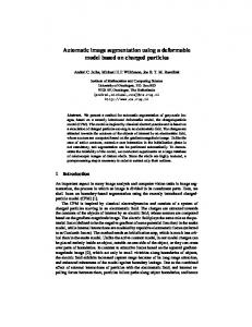
2 Review 2.1 Human visual properties- JND (Just Noticeable Difference) JND is the sensitivity of human visual system to the changes in luminance. A typical JND function is shown in 1
Figure 1, where luminance is in terms of gray level. For example, gray level 0 has a JND value of 20, indicating that human eye cannot distinguish between luminance intensities between gray level 0 and gray levels 20.
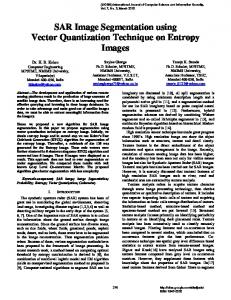
Pre-Processing
I(m,n)
S(m,n)
Smoothing
G(m,n)
Compute Gradient
Gradient Thresholding
JND Curve
20
Pre-Processing
18
GT(m,n)
16 14
R(m,n)
Visibility 12
Watershed
Region Merge
Threshold 10
8
W(m,n)
6 4 2
0
50
100
150
200
250
300
Fig.3 The Pre- and Post-processing for resolving the over-segmentation problem in watershed based segmentation.
Backgroubd Luminance
Fig.1 A Typical JND function
2.2 Watershed algorithm and the over-segmentation problem
,3
The concept of watershed originally came from geography. 7 Vincent extended the concept to digital space by applying the immersion technique. Segmentation by Watershed normally suffers from the over-segmentation problem as shown in Fig.2, a total of 3622 regions are used to represent the Lena images, which is impractical.
In this section we shall examine the effects and limits of smoothing and gradient thresholding in the pre-processing.
Effects and Limits of Pre-Processing
Effects and limits of the smoothing process Smoothing can effectively prevent the creation of insignificant regions in a watershed image GT(m,n). However, smoothing has its limits: Over-smoothing may weaken important edges, therefore, causing incomplete region representation. Figure 4 shows the watershed Cameraman with no smoothing filtering and applying a 3x3 averaging filters at gradient threshold of 80. The second (lower) tower at the rightmost side in the background is completely missing for filter 5x5. Thus, there is a trade offs between the region reduction and region incompleteness when the filter size is considered. We decide to adopt the simple 3x3 averaging filter because it yields satisfactory region reduction while preserve most important edges. and quite simple in computation. Although more sophisticated Gaussian filter 9 may be used for greater region reduction, our strategy would rely on the gradient thresholding (to be illustrated in this section) for further region reduction, because it requires much less computations than smoothing and yet very effective.
Fig.2 The over-segmentation problem. Lena(256 256) (left) and segmentation representation (3622 regions) by watershed algorithm (Right)
In order to obtain a concise region representation, pre-processing and post-processing are applied to resolve 810 the over-segmentation problem . Pre-processing (smoothing and gradient thresholding) prevents the generation of insignificant regions in the watershed process; while post-processing (Region merge) merges regions according to certain criteria for a more concise region presentation See Fig. 3. Gauch’s smoothing and gradient thresholding 2 belong to the pre-processing while Harris’s RAG (Region Adjacency Graph) region merge belongs to the post-processing.
Fig.4 Region representation for Camera(256 256) after watershed with Gth=80 and (a) Without smoothing 1873 regions, (b) with 5 5 filter, 550 regions
2
In this section, we demonstrate that over-segmentation problem can be greatly prevented by pre-processing (smoothing and gradient thresholding) before the watershed process. However, pre-processing has its limitations, region number after pre-processing is still too many for most applications. If more concise region representation is required, then post-processing (i.e. region merge) can be applied.
Effects and limits of Gradient Thresholding Increasing gradient threshold Gth may achieve greater region number reduction as shown in Figure 11. The effects of gradient thresholding on Cameraman are shown in Figure 5. Gradient thresholding is much simpler in computation than smoothing filter and yet very effective in region reduction.
3 JND Based Region Merging Region merge is the major method to further reduce the region number. Two neighboring regions can be merged into a single region if they are similar enough. Harris [8] used the RAG to find the pair of region with closest mean gray levels for merging. Which is computationally intensive. In this paper, we propose JND region merge method as follows: two neighboring regions with mean gray level of I1 and I2 are merged if |I1 – I2| < MIN (JND[I1],JND[I2])+ , where is the merge controlling factor. Why JND merge criteria? Fig. 7 shows that human perceptual sensitivity is not constant, rather, it is a function of intensity (see JND curve in Fig. 1.) =0.
(a) Gth = 40, 1454 regions (b) th=80, 740 regions Fig.5 Effects of gradient thresholding on watershed Cameraman
Figure 6 show the percentage of remaining region number in the watershed images as a function of gradient threshold for the 5 test images (Cameraman, House, Lena, Claire, and CT (Computerized Tomography)). As expected the region number drops as gradient increases. However, the decreasing rate depends on image contents. House and Clair have the steepest decreasing rate, Lena and Cameraman have moderate decreasing rate while CT has the slowest decreasing rate. 100 90
Cameraman Claire House Lena CT
80 70 60
% 50
Fig.7 (a) Tested gray image (b) Region merge using fixed threshold (c) Region Merge using JND criterion (more consistent with visual perception).
40 30 20 10 0
0
20
40
60
80
Gth
100
120
140
160
For regions with population smaller than 1% of the total pixel number is considered as small regions, which is encouraged to merge to its neighbor by adding 10 to the I1 and I2 are merged if |I1 – I2| < MIN (JND[I1],JND[I2])+ +30. Experiments show that a great percentage of regions are classified as small region.
Fig.6 Percentage of region number in watershed image as a function of gradient threshold.
Combined Effects of smoothing and gradient thresholding
5
Since region number reduction in the pre-processing is computationally more efficient than in post-processing (region merge requires significant higher computations), it is desired to reduce region number as many as possible in the pre-processing stage, yet the significant boundaries should be preserved. With 3x3 averging filter, the recommended gradient threshold is Gth=40 for Lena (to keep the weak but perceptually important hut top edges), while Gth=80 for Cameraman, Lena, House and Gth=120 for CT are safe in keeping most contents.
Experiment Results
5.1
(a)
Experiments results
=0 , 31 regions (b) =20, 13 regions (c) =40,10 regions Fig.8 House, Gth=70
3
_ _ 1, if x j ,k xk JND ( xk ) _ _ 0, if x x JND ( x ) j ,k k k
j ,k
_
x j ,k is the j th pixel of the k th region; x k is average value of all pixels of the k th region.
(a) =0, 47 regions (b) =20, 26 regions (c) =40 ,16 regions Fig.9 Cameraman(256 256), Gth=80, (a) Original (b)
A segmented image with lower JND_Variance indicates a better approximation of the original image.
5.2.2 Performance Evaluation Cameraman
28
30
24
(a) =0,15 regions (b) =20,6 regions (c) =30 ,5 regions
25
JND
20
PSNR
Variance
JND Merge Fixed Threshold Merge
20
15
18
16
JND Merge Fixed Threshold Merge
JND
22
Fig.10 Claire, Gth=80,
Cameraman
35
26
10
0
50
100
150
200
250
5
300
0
50
Region Number
100
150
200
250
300
Region Number
Fig12. Performance comparison of fixed threshold and JND merging criterion (a) JND_PSNR (b) JND_Variance
5.3.1 Comparison with Haris 2 RAG merging (b) =0, 43 regions
(a)Original
JND based segmentation result is more consistent with human visual perception, requires fewer computations, And there is no need to predetermine the region number.
(c) =40 ,11 regions
Fig.11 CT(256 256), Gth=80,
5.2 Performance Evaluation and Analysis 5.2.1 Objective Evaluation Criteria for Quality of Image Segmentation We
propose
subjective
criteria
for
evaluation
of (a)
segmentation quality as the complement to subjective evaluation by human eyes.
JND _ PSNR 10log10 N
JND _ MSE
M
2552 JND _ MSE
^
5.3.2
(1)
[ p(i, j) p(i, j) JND(i, j)]
2
(b)
(c)
Fig.13 Comparison of RAG and JND criteria (a)MIT original image (b) Using RAG merge criteria (80 regions) (c) Using JND criteria (76regions, Gth=80, =0)
Comparison with Gao’s algorithm 25
(i , j )
i 1 j 1
N M
1,
if p (i , j ) p (i , j ) JND (i , j )
0,
if p (i , j ) p (i , j ) JND (i , j )
^
(i , j )
^
N, M is the length and width of the image ; p(i, j ) is ^ gray-level value of pixel (i,j); p(i, j ) is the average gray-level value after segmentation; JND(i, j ) is the visibility threshold of the pixel (i,j)。 A segmented image is obtained by assigning each pixel with region’s average gray-level. A segmented image with higher JND_PSNR indicates a better approximation of the original image. Nk
JND _ Variance
Nj
[ x k 1 j 1
_
j ,k
Fig.14 (a)Claire original (b)Gao’s result
Note that eyes are missing in Gao’s result.
6
Conclusion
In this paper, we adopt JND human visual properties for resolving the over-segmentation problem of watershed. Experiments and analysis show that not only the segmented representations are more concise and conform to human perception, but also the computational load is greatlt reduced than Harris [2] and Gao’s [25] method. The JND approach produces robust segmentation to various type of images.
_
xk JND( xk )] j ,k
(c)JND,10 regions
(2)
Nk
4
References
21.
1. Qian Huang and Dom, B ,1995 , Quantitative methods of evaluating image segmentation , IEEE Proceedings., International Conference on Image Processing, Vol. 3 , pp. 53 -56 2. K. Haris, S. N. Efstratiadis, and N. Maglaveras andA.K Katsaggelos, “Hybrid Image Segmentation Using Watersheds and Fast Region Merging”, IEEE Trans. Image Processing, vol.7, no.12, pp.1684-1699, Dec.1998 3. K. Mardia and T. Hainsworth ,” A Spatial Thresholding method for image segment -ation ” ,IEEE Trans. Pattern Anal. Machine Intell,vol.10,pp919-927, Nov.1998 4. J.Canny, “A Computational approach to edge detection”, IEEE Trans. Patterm Anal. Machine. Intell, vol. PAMI-8, pp.679-698, Nov. 1986 5. Wei-Ying Ma and B. S . Manjunath ,”EdgeFlow: A technique for boundary detection and image segmentation”,IEEE Trans. Image Processing, vol.9 ,No.8, pp1375-1388, August 2000 6. S. Chen, W. Lin and C. Chen ,” Split-and-merge image segmentation based on localized feature analysis and statistical tests”,CVGIP: Graph. Models Image Process, vol.53, pp.457-475 ,Sept. 1991 7. L. Vincent, and P. Soille, “Watershed in Digitl Spaces : An Efficient Algorithms based Immersion Simulations”, IEEE Trans. Pattern Anal. Machine Intell., vol.13 ,June 1991, pp.533-598 8. D. Wang, “ A Multiscale gradient algorithm for image segmentation using watersheds”, Pattern Recognition , vol.678,no.12, pp.2043-2052, Jan.1997 9. J. M. Gauch, “Image Segmentation and Analysis via Multiscale gradient watershed hierarchies”, IEEE Trans. Image Processing, vol.8,no.1, pp.69-79, Jan.1999 10. M. W. Hansen and W. E. Higgins, “Watershed-based Maximum Homogeneity filtering”,IEEE Trans. Image Processing, vol.8, no.7, pp.982-988, July 1999 11. L. Shafarenko, M. Petrou and ,J. Kittler,”Automatic watershed segmentation of randomly textured color images”,IEEE Trans. Image Processing, vol.6, no.11, pp.1530-1544, Nov.1997 12. Alina N. Moga and Moncef Gabbouj,”Parallel Image Component Labeling with Watershed Transformation”,IEEE Trans. Pattern Analysis and Machine Intelligence, vol.19, no.5, pp.441450, May.1997 13. Laurent Najman and Michel Schmitt,”Geodesic Saliency of Watershed Contours and Hierarchical Segmentation”, IEEE Trans. Pattern Analysis and Machine Intelligence, vol.18, no.12, Dec. 1996 14. R. Dubes and A. Jain,”Random filed models in image analysis”, J.Appl. Stat, vol.16, pp.131-164 ,1989 15. Anjan Sarker,Manoj K. Biswas, and K.M.S. Sharma,”A Simple Unsupervised MRF Model Based Image Segmentation Approach”, IEEE Trans. Image Processing, vol.0, no.5, May. 2000 16. Jaesang Park and James M. Keller,”Snakes on the Watershed “, IEEE Trans, Pattern Analysis and Machine Intelligence, vol.23, no.10, Oct. 2001 17. T. Pavlidis and Y. Liow, “Integrating region growing and edge detection “,IEEE Trans. Pattern Anal. Machine Intell.,vol. 12, pp.225-233, Mar. 1990 18. F. Meyer and S. Beucher,” Morphological segmentation”, J. Vis. Commun. Image Represent, vol.1, pp.21-46, Sept,1990 19. Chun-Hsien Chou and Yun-Chin Li , “ A Perceptually Tuned Subband Image Coder Based on the Measure of Just-Noticeable-Distortion Profile “, IEEE Trans. On Circuits and System for Video Technology. Vol. 5, No. 6, December 1995. 20. Yu Jin Zhang,” A review of recent evaluation methods for image segmentation”, IEEE Tran. Signal Processing,
22. 23. 24.
25.
26.
27.
28. 29
5
pp.148-151, 2001 Brendan McCane,”On the evaluation of image segmentation algorithms”, Oct,1997 Rafael C. Gonzales & Richard E. Woods , “ Digital Image Processing “ ,1996 Fuhui Long, Dagan Feng, Hanchuan Peng and Wan-Chi Siu,” Extracting Semantic Video Objects”,IEEE Computer Graphics and Application, pp.48-55, Jan. 2001 Jae Gark Choi,Si-Woong Lee, and Seong-Dae Kim,”Spatio-Temporal Video Segmentation Using a Joint Similarity Measure”, IEEE Trans, Circuits and Systems for Video Technology, vol.7, no.2, APRIL. 1997 Hai Gao, Wan-Chi Siu, and Chao-Huan Hou,”Improved Techniques for Automatic Image Segmentation ”,IEEE Trans. Circuits and System for Video Technology. Vol.11, no.12, DEC. 2001 Giancarlo Iannizzotto and Lorenzo Vita ,“Fast and accurate edge-based segmentation with no contour smoothing in 2-d real images “, IEEE trans. Image Processing ,vol. 9, no.7,July 2000 J.M. Gauch and S.M. Pizer , “Multi-resolution analysis of ridges and valleys in Grey-scale images” , IEEE Trans. Pattern Anal. Machine Intell., vol. 15 , no. 6, pp.635-646, 1993. P. T. Jackway. “Gradient watersheds in morphological scale-space”, IEEE Trans. Image Processing, vol. 5, no.6, pp913-921, 1996. A.S. Wright and S.T. Acton,”Watershed pyramid for edge deyection”,IEEE Proceedings.Image processing, vol. 2,pp. 578-581, 1997.