LaboImage: a Workstation Environment for Research in Image Processing and Analysis
Alain Jacot-Descombes(1), Krassimir Todorov(1), Denis F. Hochstrasser(2), Christian Pellegrini(1) and Thierry Pun(1)
(1)
Centre Universitaire d’Informatique (C.U.I.) Faculty of Sciences, University of Geneva 12, rue du Lac CH-1207 GENEVE SWITZERLAND electronic mail:
[email protected] (2)
Numeric Imaging Group Center for Hospital Informatics Geneva University Hospital CH-1211 GENEVE 4 SWITZERLAND
Corresponding author: Alain Jacot-Descombes.
Computer Applications in the Biosciences. Vol 7, no 2, 1991, pp 225-232
1
Abstract Numerous images are produced daily in biomedical research. In order to extract relevant and useful results, various processing and analysis steps are mandatory. The present paper describes a new, powerful and user-friendly image analysis system: LaboImage. In addition to standard image processing modules, LaboImage also contains various specialized tools. These multiple processing modules and tools are first introduced. A 1-D gel analysis method is then described. The new concept of “normalized virtual 1-D gel” is introduced, making in particular comparisons amongst gels easy. This normalized gel is obtained by compensating for the bending of the lanes automatically; no information loss is incurred in the process. Finally, the model of interaction in a multi-window environment is discussed. LaboImage is designed to run in two ways: interactively, using menus and panels, and in batch mode by means of userdefined macros. Examples are given to illustrate the potentialities of the software. Keywords: image processing, image analysis, 1-D gel analysis, normalized gel, interaction, multi-windows environment.
2
Introduction Biomedical sciences are a domain where images play a crucial role. In order to analyse them in detail, scientists must often rely on specialized equipment. Computers are sometimes simply used to produce a displayed image with a contrast sharper than the original one, by remapping grey levels (Wesley and Wallenslager, 1986; Lutz et al, 1990, to be published). Many other types of processing can however be performed, such as enhancement, filtering, edge detection, mathematical transformation and so on (Rosenfeld and Kak, 1982; Gonzales and Wintz, 1987). Typical biomedical applications are the search for contours in vascular networks (Collorec and Coatrieux, 1988), the enhancement of chest radiographs (Daponte and Fox, 1988) and cell counting (Preston and Bartels, 1988). In this context, LaboImage is an image analysis software providing users with a large choice of processing procedures in a user-friendly environment. LaboImage is not dedicated to a specific task, but allows the user to solve a large number of different problems. Specialized tools are also included for more specific matters. LaboImage is typically suited to exploratory research, where one tries to compare different methods. This software has been distributed in various computer centers and universities over the world, and is also used as a platform for an image analysis course given for computer science students at University of Geneva.1 Other softwares also provide environments for image processing, for example (Groen et al, 1988; McEachron et al, 1989; Vernon and Sandini, 1988). They are often dedicated to specific classes of images, such as 3D medical images (Robb et al, 1989). Compared with these other softwares, LaboImage tries to provide as general as possible a platform for various scientific investigations, while still offering a few selected, specialized tools. Different approaches are thus available to rapidly determine and evaluate solutions to a given problem. The main advantage of LaboImage lies precisely in this integration of standard processing methods (such as filters, transforms, etc.) together with particular tools. As a typical application, it is possible to take an input image of a gel, filter it to remove acquisition noise, then perform a 1-D gel analysis. The results are kept within LaboImage, allowing for example comparison of several processed gels by arithmetic subtraction. In the “Algorithm” section, we survey the large choice of processing families and the kind of data this software can process. We also enumerate the specific tools. A section is then
1. LaboImage is provided free of charge for academic users; interested persons should contact the author.
3
dedicated to the 1-D gel analysis tool which is presented in detail. In the “Implementation of interaction” section, we first explain the underlying interaction concepts on which LaboImage is built. We then discuss the different interactive manners for using LaboImage. A simple example finally illustrates a typical working session.
System and methods LaboImage presently runs on Sun™ workstations (SUN 3/xxx and SUN 4/xxx) in the SunView windowing system. An adaptation to more standard windowing and interfacing systems is also planned (e.g. X-Window System™ (Scheifler et al, 1988), OSF/Motif™ (Open Software Foundation, 1990)). The software is written in the C language (Kernighan and Ritchie, 1978); it is about 50000 lines long. The executable code uses approximately 2 Megabytes.
Algorithm Standard processing and data LaboImage is currently comprised of over one hundred operators. They can be grouped in different families, according to their utility and complexity. The most basic operations consist in retrieving an image from mass storage, displaying it and saving it after some processing.However, visualization of images is not the only purpose of such a software. The following list briefly describes the classes of operations as presently implemented; the specialized tools are presented in the next paragraph. • Display:
one or eight-bit depth rasters. A threshold at the mean value with or without error distribution (Floyd-Steinberg algorithm, Foley et al, 1990) is used for one bit display; linear or logarithmic grey levels and color (RGB) with or without error distribution are used for eight-bit displays. Postscript™ (Adobe Systems Incorporated, 1985) files can also be generated from the images.
• Storage:
scalar, complex or color (RGB) images are saved on mass storage in the LaboImage format (see below) or in the Sun raster format.
• Retrieval:
images in the LaboImage format, Sun raster format and other specific formats can be loaded.
4
• Geometry:
operations such as rotation, translation, transposition, scaling and symmetry.
• Histogram:
grey level histograms can be computed, displayed and printed.
• Data type conversions:
type conversion between the following image types: binary, byte, short, integer, real, cartesian and polar complex. This gives the possibility of modifying grey level scales as well as of trimming the higher and lower parts of the distribution during conversion.
• Arithmetic operations:
the four basic arithmetic operations are implemented, (i.e., addition, subtraction, multiplication and division) with a scalar constant and a scalar image, between two scalar images and using complex images.
• Logical operations:
NOT, AND, OR, XOR between binary images.
• Measures:
some morphological measurements can be directly performed on the displayed images, such as grey level density profiles; statistical measurements can be computed in regions of interest.
• Transformations:
regular and optical Fourier transformation, direct and inverse.
• Convolution:
users can extract part of an image or define a mask, to be convolved or correlated with any other image.
• Edge detection:
typical operators such as Sobel, Roberts, Laplacian, Frei and Chen, zero crossing and peak following.
• Enhancement:
different methods such as histogram equalization, median and high pass filter, Gaussian and Hamming filter, edge preserving smoothing.
• Segmentation:
thresholding, regions segmentation methods such as split and merge, recursive segmentation (Ohlander, Price and Reddy, 1978) and region growing.
• Noise generator:
uniform and gaussian noise can be generated and added to images.
• Binary morphology:
all the basic and complex operations of mathematical morphology are implemented in an hexagonal raster (Serra, 1982).
• Grey level morphology: dilation, erosion, opening and closing with different structuring elements or image parts (Coster and Chermant, 1985).
5
The previous list of processing families gives a general view of the software. In fact, many operators allow free choice of parameters, thereby increasing the actual number of available methods. In addition to these processing methods, some basic utilities are included, such as image padding or color to grey level transformations. As can be deducted from the above list of processings families, various types of informations are manipulated by LaboImage. Data are stored using two different kinds of arrays: vectors and images planes. The following table summarizes the data structures used by the software (Table 1).
[ Insert table 1 ] N image planes and N vectors are simultaneously available in central memory, numbered from 0 to N-1. N is currently set to 10, but there is no limit to either the number or size of these data structures. Images as well as color tables can be saved on disk. A color table is saved as a file of 3 times 256 bytes, each of the 256 colors being defined by a triplet of red, green and blue. Images are stored on disk in the LaboImage format, i.e., using two files: one containing the image data, the other one storing various pieces of descriptive information (Table 2).
[ Insert table 2 ] Specialized tools This paragraph briefly enumerates the more specific processing tools available in LaboImage. The 1-D gel analysis tool is described in detail in the next section. • a help tool, which gives on-line explanations about the operations being performed; • an interactive color table manipulation tool, which allows the definition of complete look-up tables with RGB or HLS representations (Lutz et al, 1990, to be published); • an image generation tool for making simple monochrome and grey level images of any size; • a tool for counting regions defined by their contours or by their grey level values; • a tool for pixel by pixel correction of an image, making use of a magnifying glass. This, for example, gives the possibility of closing region contours before counting; • an expert system for guiding image segmentation (Hu et al, 1990); • a tool for analysing 1-D gel autoradiograms (see the next section);
6
• a tool for comparing images in a sequence. For example, the grey level evolution of a specific region can be measured; • a tool for interactive creation and execution of macros (see the “Implementation of interaction” section). LaboImage is constantly evolving; new tools are regularly being added.
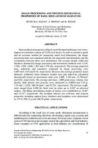
The 1-D gel analysis tool Overview The purpose of the 1-D gel analysis tool (gel1D-tool) is to automatically determine the density profiles as well as the profile peaks for one dimensional gels. The system can be used for analyzing any type of 1-D gel, e.g. autoradiograms (Figure 1), Coomassie Blue or silver stained profiles. The only parameter which is required from the user is the number N of lanes (e.g. 11 in Figure 1).
[ Insert fig 1 ] The first steps of the method are based on an approach fully described in (Pun et al., 1985); they are summarized below. However, two new elements have been added, making quantisation more precise and comparisons between gels much easier. The first addition relates to the determination of the lane boundaries. The imprecision due to the third degree polynomial fit over the gel boundaries is compensated for and no information is lost. The second addition concerns the construction of a “normalized virtual 1-D gel”. This new representation allows in particular an easy comparison between gels. Determination of the profiles is performed in two stages. The first locates the lane boundaries; the second computes the profiles for each lane, finds the peaks in these density profiles and determines the “normalized 1-D gel”. Determination of the lane boundaries In the following explanations i and j are respectively the horizontal and the vertical coordinates in the image, g(i,j) the grey level of the pixel located at the coordinates i and j, SizeI and SizeJ the image size in both directions. Lane denotes a 1-D lane in the gel, and column means a column of grey level pixels in the image.
7
Location of the lane boundaries is done in two steps: a pre-estimation of their position is first performed, which is then followed by a more precise estimation. For the pre-estimation, each lane is considered to be a straight vertical zone whose left and right limits are to be determined. The grey levels from all the pixels in each column of the image are first added together. This yields one cumulated grey level function for the whole image, where each value CumGreyLevel(i) corresponds to one image column: SizeJ
CumGrayLev ( i ) =
∑
g ( i , line ) ; i = 1…SizeI
(equation 1)
line = 1
An extremum filter followed by a sliding t-test are then performed over that cumulated grey level function (de Souza, 1983). The extremum filter replaces the value of the center element in a window of size m by the largest (or smallest) value in that window. The largest value is chosen if it is closer than the smallest to the center value. The effect of this filter is to provide a modified cumulated grey level function with large plateaus of constant values. The sliding t-test will then detect transitions. In a window of size 2m+1, it compares the average of the m leftmost values l(i) to the average of the m rightmost ones r(i), using their normalized difference t(i): t(i ) = ( l (i ) − r(i ) ) ⁄ s(i )
(equation 2)
where: l (i ) = r(i ) =
s(i ) =
i−1
∑
k = i−m
i−1
∑
k = i−m
i+m
∑
k = i+1
CumGrayLev ( k ) ⁄ m
(equation 3)
CumGrayLev ( k ) ⁄ m
(equation 4)
2
( CumGrayLev ( k ) ) − l (i ) + 2
i+m
∑
2
2
( CumGrayLev ( k ) ) − r(i )
k = i+1
m ( m − 1)
(equation 5) The parameter m defining the window sizes of these two operators (extremum filter and sliding t-test) is chosen as a function of the number N of lanes in the image: m =
SizeI 2⋅N
(equation 6)
8
Lane boundaries correspond to positions i where |t(i)| is the largest. A maximum of t(i) corresponds to a left boundary of a lane (LeftBoundary), a minimum of t(i) corresponds to a right boundary (RightBoundary). This gives a pre-estimation of the lane positions. At this stage, we only have as many pairs of boundary coordinates as there are lanes in the image, i.e. N. We need now to refine this pre-estimation in order to have N pairs of boundary coordinates per line in the autoradiograph: this will give us the complete lane boundaries. For the precise determination of the lane boundaries, the locus of the lane axis is first computed. Then, for each lane, on each side of the axis, precise boundaries will be found. The pre-estimated lanes are scanned line by line For each line, the center of the current lane is the center of gravity of the pixel values, computed between the pre-estimated boundaries. Thus, for image line j and for each of the N lanes: RightBoundary n
∑
CenterColumn n(j ) =
i ⋅ g ( i, j )
LeftBoundary n RightBoundary n
∑
; n = 1…N
(equation 7)
g ( i, j )
LeftBoundary n
Here LeftBoundaryn and RightBoundaryn denote pre-estimated boundaries in the n-th lane as described above. For each lane, the locus of the lane axis is finally approximated by a third degree polynomial. Having these axes, the precise boundaries can be found using the fact that between two axes there are exactly one right boundary and one left boundary. A sliding t-test is again applied, but this time for each line of the image. The minima and maxima found between two axes are respectively the precise left and right boundaries for the two adjacent lanes. A third degree polynomial fit is finally done over the boundary points, yielding the precise boundaries (Figure 1). As we can see in Figure 1, a lane is not exactly confined within its boundaries. According to the old method (Pun et al., 1985), the overflowing part was ignored. In order to have an integration of the complete profile, this overflowing part is now uniformly distributed inside the boundaries. Computing the virtual normalized gel and the density profiles Once the boundaries are known, the profiles and peaks can be evaluated. It is then possible to determine the “normalized virtual 1-D gel” representation. The gel is normalized in the sense that the geometric variations of the lanes have been corrected; comparisons between gels is
9
now possible by simple superposition. For example, several gel images can be processed, yielding several normalized gels; these can be compared by using subtraction. For each lane, the profiles are computed by averaging the grey level values along normals to the central axis. This allows correct treatment of slightly curved lanes. Each lane n has its own profile, represented as a vector of real numbers Pn(j). Those numbers give for each lane n the quantity of substance at vertical position j. Finally, the virtual normalized gel is reconstructed using those profiles (Figure 2). It represents an image of the same size as the original. All the lanes have the same width and the inter-lane spacing are considered as being uniformly white. Each normalized lane has constant horizontal values given by the density profile Pn(j).
[ Insert fig 2 ] Determination of the peaks of the density profiles is performed using the second derivative of Pn(j). The regions in the profiles where this derivative is greater than zero are considered as belonging to a peak. In order to decrease the effect of noise, the profiles can be smoothed using an averaging filter. Also, peaks whose area or amplitude is below some user specified threshold can be ignored. Once the peaks are known, the program asks the user to specify the quantity of substance in each lane; the quantity in each peak can then be evaluated (Figure 3).
[ Insert fig 3 ] The boundaries of the lanes, the profiles, the virtual normalized gel and the peaks can all be displayed and, if needed, manually modified. All the results can be saved into a file, which can be processed later by other programs or again reloaded into LaboImage.
Implementation of interaction Method of interaction This section describes the general principle of interaction used in the software. LaboImage is built on top of a so-called notification-based system; the difference between such a system and a conventional program is presented below. In a classical program, all components reside in the what is called the application part. This means that the control loop, the interface with users and the general flow of processing are
10
defined in advance and cannot be altered (Figure 4).
[ Insert fig 4 ] Such a scheme is typical of a command interpreter. The software first reads the command; if it is a quit request, the program terminates execution, otherwise parameters are read and the process corresponding to this input is executed. In a notification-based system, the control loop is moved from the application part to the so called notifier, which reads the events and calls the corresponding procedure. This scheme is the underlying structure of LaboImage (Figure 5). The full menu system with procedures
[ Insert fig 5 ] associated with each item is first constructed in the application part, then control is passed to the notifier. From that moment, the user is just sending events to the notifier by choosing items with the mouse. The notifier then analyses the received events and possibly calls an interface procedure to ask for parameters. This is done using a panel. In this case, the notifier receives the parameters from the keyboard as events and sends them to the interface procedure. The correct processing procedure is finally called; after termination, control is returned to the notifier. In summary, a classical program only allows for a very linear flow of operations that is controlled by the program. On the other hand, the flow of execution of a notifier based program is not predetermined, and is controlled by user requests (through menus and mouse). User interface LaboImage can run in two modes: interactive or automatic. In the first mode, the software is driven by a menu system attached to each button of the master window and giving users a hierarchical list of processing procedures and tools (Figure 6).
[ Insert fig 6 ] Desired items are selected with the mouse. If the chosen processing requires parameters, specific pop-up panels are opened, asking the user for the missing information. Parameters are very often the numbers of source and destination image planes, i.e. the image on which the processing is made and the one on which to store the result. Sometimes parameters specific to an operation are required, for example an angle of rotation in a geometrical transform. During the entire session, a trace of all the operations appears in the master window and is simultaneously written in a log-file.
11
In the automatic mode, another kind of data (called macro) is used to control the sequence of processings. A macro is a set of operations that are to be applied sequentially. Making a parallel with computer programming, we can say that macros are like programs. We can simultaneously have up to M macros in central memory, numbered from 0 to M-1 (M is 10 in the current implementation). They are written on disk in ASCII format. A tool called Macrotool is included in LaboImage; it allows the creation and manipulation of such macros. For creation, the user chooses items with the menu system and introduces parameters as in the interactive mode; however, no processing is executed at this stage, but the data structure for the current macro is created and updated. After this, macros can be run in different ways: • Fully automatic:
the macro is executed as it is, without any changes, i.e. without interaction. This means that the set of instructions is executed exactly with the same parameters as in the recorded macro.
• Fully manual:
confirmation is required for all parameters.
• Images numbers:
only numbers of source and destination planes are required.
• Parameters:
only specific parameters are required; plane numbers are those initially stored.
A simple example of utilization Edge extraction on a bacterial cell image is given below as a simple processing application. This example is performed interactively by choosing all operations with the menu. The first step is to load the image to be processed into the system. This is made by the “Acquisition” menu: the image is stored into one of the N buffers. We then decide to apply a median filter for noise reduction purposes. After this, we choose the Roberts operator followed by the peak following method in order to obtain edges. We finally want to visualize both the original and resulting images. Figure 7 shows the master window together with both images; the master window contains the trace of operations. If the result is not satisfying, we can take an intermediate image at any stage of the process and try other operations.
[ Insert fig 7 ] Once a satisfying set of processing procedures is found, we can create a macro by using the same menu system. It allows us to manipulate a set of processing steps as a single entity. This macro can later be executed automatically without interaction or just by changing some parameters, as explained in the previous section. The same result as in the interactive mode will
12
be obtained. Figure 8 shows the tool for manipulating macros. The displayed macro is the same set of processing steps as used above to extract edges from the bacterial cell image.
[ Insert fig 8 ] Discussion Digital image processing and analysis is very useful for processing various scientific images, but powerful and user-friendly softwares have also to be available for non-specialized users. LaboImage is an answer to such a need. It provides researchers with various image processing methods through an easy-to-use interface. The major advantage of such a software is its large variety of processing procedures and specialized tools: many different problems can be solved using a unique system. It also provides the possibility comparing various methods and of designing well adapted solution. The 1-D gel analysis tool is an example of how useful LaboImage can be. Finally, we emphasize the implementation model which clearly separates the interface part of the system from the processing one. This conception allows easy adaptation of LaboImage to new theoretical methods or practical tools.
Acknowledgment This paper is the result of a research development by the vision group of C.U.I., University of Geneva. We gratefully acknowledge the work done by all researchers and students actively involved in this project, in particular R.W. Lutz. We would like also to thank the Medical Imaging Group of Geneva University Hospital for its collaboration.
13
References Adobe Systems Incorporated (1985) PostScript Language Reference Manual. Addison-Wesley Publishing Company, Reading, MA. Collorec, R.; Coatrieux, J. L. (1988) Vectorial Tracking and Directed Contour Finder for Vascular Network in Digital Subtraction Angiography. Pattern Recognition Letters, 8, 353358. Coster, M.; Chermant, J.-L. (1985) Précis d’Analyse d’Images. Editions du Centre National de la Recherche Scientifique, Paris. Daponte, J. S.; Fox, M. D. (1988) Enhancement of Chest Radiographs with Gradient Operators. IEEE Transactions on Medical Imaging, 7 (2), 109-117. de Souza, P. (1983) Edge detection using sliding statistical tests. Computer Vision, Graphics, and Image Processing, 23 (1), 1-14. Foley, J. D.; Van Dam, A.; Feiner, S. K.; Hughes, J. F. (1990) Computer Graphics: principles and practice. Second edition. Addison-Wesley Publishing Company, Reading, MA. Gonzalez, R. C.; Wintz, P. (1987) Digital Image Processing. Addison-Wesley Publishing Company, Reading, MA. Groen, F. C. A.; Ekkers, R. J.; De Vries, R. (1988) Image Processing With Personal Computers. Signal Processing, 15 (3), 279-291. Hu, Z. P.; Pun, T.; Pellegrini, C. (1990) An Expert System for Guiding Image Segmentation. Computerized Medical Imaging and Graphics, 14 (1), 13-24. Kernighan, B. W.; Ritchie, D. M. (1978) The C Programming Language. Prentice-Hall, Englewood Cliffs, New Jersey. Lutz, R. W.; Pun, T.; Pellegrini, C. (1990, accepted for publication) Colour Displays and Lookup Tables: Real Time Modification of Digital Images. Computerized Medical Imaging and Graphics. McEachron, D. L.; Hess, S.; Knecht, L. B.; True, L. D. (1989) Image Processing for the Rest of us: the Potential Utility of Inexpensive Computerized Image Analysis in Clinical Pathology and Radiology. Computerized Medical Imaging and Graphics, 13(1), 3-30. Ohlander, R.; Price, K.; Reddy, D. R. (1978) Picture Segmentation Using a Recursive Splitting Method. Computer Graphics and Image Processing, 8, 313-333.
14
Open Software Foundation (1990) OSF/Motif™ Programmer’s Reference. Prentice-Hall, Englewood Cliffs, New Jersey. Preston, Jr., K.; Bartels, P. H. (1988) Automated Image Processing for Cells and Tissue. In: Newhouse, V. L. (ed). Progress in Medical Imaging. Springer-Verlag New York Inc., pp 1121. Pun, T.; Trus, B.; Grossman, N.; Leive, L.; Eden, M. (1985) Computer Automated Lanes Detection
and
Profiles
Evaluation
of
One-dimensional
Gel
Electrophoretic
Autoradiograms. Electrophoresis, 6 (6), 268-274. Robb, R. A.; Hanson, D. P.; Karwoski, R. A.; Larson, A. G.; Workman, E. L.; Stacy, M. C. (1989) Analyze: A Comprehensive, Operator-Interactive Software Package for Multidimensional Medical Image Display and Analysis. Computerized Medical Imaging and Graphics, 13 (6), 433-454. Rosenfeld, A.; Kak, A. C. (1982) Digital Picture Processing. 2nd Edition. Academic Press, New York. Scheifler, R.; Gettys, J.; Newman, R. (1988) X-Window System™ C Library and Protocol Reference. Digital Press. Serra, J. (1982) Mathematical Morphology and Image Analysis. Academic Press. Vernon, D.; Sandini, G. (1988) VIS: A Virtual Image System for Image-Understanding Research. Software - Practice and Experience, 18 (5), 395-414. Wesley Davis, G.; Wallenslager, S. T. (1986) Improvement of Chest Region CT Images Through Automated Gray-Level Remapping. IEEE Transactions on Medical Imaging, MI5 (1), 30-34.
15
List of tables Table 1 Available data structures. Table 2 The two files defining an image.
16
Images
binary, byte, short, integer, float
1 plane
complex
2 planes
color (RGB)
3 planes
Histogram
1 vector
Table 1
17
Descriptive file:
type of image elements(T) number of rows (R) number of columns (C) minimum, maximum, average and standard deviation for each plane date and time of image creation comments
Image file:
R x C elements of type T
Table 2
18
List of Figures Fig. 1
Original image of 1-D gel (11 lanes), on which are superimposed the lane boundaries automatically extracted by the proposed method.
Fig. 2
Virtual normalized gel and density profiles obtained from Fig. 1.
Fig. 3
Original gel together with the profile of lane 1. The peaks are indicated in black, and are numbered sequentially from top to bottom.
Fig. 4
Flow chart of a conventional program
Fig. 5
Scheme of LaboImage, based on a notification system.
Fig. 6
The master window with its attached menu system (a bilingual English and French implementation is available).
Fig. 7
A session example with LaboImage. The master window displays all operations executed to extract edges from the bacterial cell image (original image from: E. Kellenberger, in: “Molecular Biology of the Cell” by B. Alberts, D. Bray, J. Lewis, M. Raft, K. Roberts, J. D. Watson. Garland Publishing Inc., 1983; reused with permission).
Fig. 8
The tool for manipulating macros. The displayed macro corresponds to the operations of Fig. 7. The name of each macro depends on the place where it stands in the menu system. For example, I_OLIMSTD is “I/O” operation, “load image”, “standard” format.
19
Figure 1
20
Figure 2
21
Figure 3
22
APLICATION
begin
Interface read command
Processing process command
Control Loop no
command=quit? yes
end
Figure 4
23
APLICATION
NOTIFIER
begin construction of menu system + master window
read event
transfer control to the notifier
mouse keyboard
call appropriate procedure for the received event
end Control Loop Interface
quit request? no
procedure 1 ... procedure m
yes
Processing procedure 1 ... procedure n
Figure 5
24
Figure 6
25
Figure 7
26
Figure 8
27