Abstract Delta Modeling

Abstract Delta Modeling Software Product Lines and Beyond

Proefschrift

ter verkrijging van de graad van Doctor aan de Universiteit Leiden, op gezag van Rector Magnificus Prof. Mr. C.J.J.M. Stolker, volgens besluit van het College voor Promoties te verdedigen op woensdag 12 november 2014 klokke 11:15 uur

door

Michiel Helvensteijn geboren te Voorburg in 1986

Promotor Prof. Dr. F.S. de Boer

(Universiteit Leiden)

Copromotor Dr. D. Clarke

(Uppsala Universitet)

Promotiecommissie Prof. Dr. F. Arbab Dr. M.M. Bonsangue Prof. Dr. R. Hähnle Prof. Dr. J.N. Kok

(Universiteit Leiden) (Universiteit Leiden) (Technische Universität Darmstadt) (Universiteit Leiden)

The work in this thesis has been carried out at Centrum Wiskunde & Informatica and Leiden University, and under the auspices of the research school IPA: Institute for Programming research and Algorithmics. The research was partially funded by the EU project FP7-231620 HATS: Highly Adaptable and Trustworthy Software using Formal Models Copyright © 2014 by Michiel Helvensteijn (www.mhelvens.net) Cover design and artwork by Tim Hengeveld (www.timhengeveld.com) Typeset with XELATEX Printed by Ipskamp Drukkers BV Published by Michiel Helvensteijn ISBN: 978-90-822936-0-9 IPA Dissertation Series 2014-14

Contents

Contents

i

1 Introduction 1.1 Problem Statement . . . . . . . . . . . . . . . . 1.2 Existing Approaches . . . . . . . . . . . . . . . 1.3 The Abstract Delta Modeling Approach . . . . 1.4 A Running Example: The Editor Product Line 1.5 Papers & Chapters . . . . . . . . . . . . . . . . 1.6 Typographic Conventions . . . . . . . . . . . . 1.7 Mathematical Preliminaries . . . . . . . . . . .

. . . . . . .

. . . . . . .

. . . . . . .

. . . . . . .

. . . . . . .

. . . . . . .

. . . . . . .

. . . . . . .

. . . . . . .

2 4 5 6 7 10 16 18

2 Algebraic Delta Modeling 2.1 Introduction . . . . . . . . . . . . . 2.2 Deltas & Products . . . . . . . . . 2.3 The Software Deltoid . . . . . . . . 2.4 The Semantics of Deltas . . . . . . 2.5 Delta Refinement and Equivalence 2.6 Delta Algebras . . . . . . . . . . . 2.7 Classification of Deltoids . . . . . . 2.8 Encoding Related Approaches . . . 2.9 Conclusion . . . . . . . . . . . . . 2.10 Related Work . . . . . . . . . . . .

. . . . . . . . . .

. . . . . . . . . .

. . . . . . . . . .

. . . . . . . . . .

. . . . . . . . . .

. . . . . . . . . .

. . . . . . . . . .

. . . . . . . . . .

. . . . . . . . . .

. . . . . . . . . .

. . . . . . . . . .

. . . . . . . . . .

. . . . . . . . . .

. . . . . . . . . .

. . . . . . . . . .

. . . . . . . . . .

30 31 36 39 44 47 48 56 60 64 64

3 Delta Models 3.1 Introduction . . . . . . . . . . . . 3.2 The Delta Model . . . . . . . . . 3.3 A Conflict Resolution Model . . 3.4 A Fine Grained Software Deltoid 3.5 Ambiguous Delta Models . . . . 3.6 Nested Delta Models . . . . . . . 3.7 Conclusion . . . . . . . . . . . . 3.8 Related Work . . . . . . . . . . .

. . . . . . . .

. . . . . . . .

. . . . . . . .

. . . . . . . .

. . . . . . . .

. . . . . . . .

. . . . . . . .

. . . . . . . .

. . . . . . . .

. . . . . . . .

. . . . . . . .

. . . . . . . .

. . . . . . . .

. . . . . . . .

. . . . . . . .

. . . . . . . .

68 69 73 75 82 88 90 93 93

4 Product Lines 4.1 Introduction . . . . . . . . . . . . . . . . . . . . . . . . . . . . . 4.2 Feature Modeling . . . . . . . . . . . . . . . . . . . . . . . . . .

96 97 99

i

. . . . . . . .

ii

CONTENTS 4.3 4.4 4.5 4.6 4.7 4.8

Product Line Implementation Product Line Specification . . Parametric Deltas . . . . . . Nested Product Lines . . . . Conclusion . . . . . . . . . . Related Work . . . . . . . . .

. . . . . .

. . . . . .

. . . . . .

. . . . . .

. . . . . .

. . . . . .

. . . . . .

. . . . . .

. . . . . .

. . . . . .

. . . . . .

. . . . . .

. . . . . .

. . . . . .

. . . . . .

. . . . . .

. . . . . .

. . . . . .

. . . . . .

102 106 109 114 116 116

5 LATEX Meets Delta Modeling 5.1 Introduction . . . . . . . . . . . . . . . . . . . . . . . 5.2 delta-modules: Deltas for Document Generation 5.3 pkgloader: An ADM-based Package Manager . . . 5.4 Conclusion . . . . . . . . . . . . . . . . . . . . . . . 5.5 Related Work . . . . . . . . . . . . . . . . . . . . . .

. . . . .

. . . . .

. . . . .

. . . . .

. . . . .

. . . . .

118 119 120 126 131 132

6 Delta Logic 6.1 Introduction . . . . . . . 6.2 A Multimodal Language 6.3 Kripke Frames . . . . . 6.4 Kripke Models . . . . . 6.5 Conclusion . . . . . . . 6.6 Related Work . . . . . .

. . . . . .

. . . . . .

. . . . . .

. . . . . .

. . . . . .

. . . . . .

. . . . . .

. . . . . .

. . . . . .

134 135 136 136 142 147 147

7 Delta Modeling Workflow 7.1 Introduction . . . . . . . . . . . . . . . . . . . . . 7.2 The Subfeature Relation . . . . . . . . . . . . . . 7.3 Locality . . . . . . . . . . . . . . . . . . . . . . . 7.4 Workflow Description . . . . . . . . . . . . . . . 7.5 The Abstract Behavioral Specification Language 7.6 The Fredhopper Access Server . . . . . . . . . . . 7.7 Conclusion . . . . . . . . . . . . . . . . . . . . . 7.8 Related Work . . . . . . . . . . . . . . . . . . . .

. . . . . . . .

. . . . . . . .

. . . . . . . .

. . . . . . . .

. . . . . . . .

. . . . . . . .

. . . . . . . .

. . . . . . . .

148 149 150 151 152 155 161 163 163

8 Dynamic Product Lines 8.1 Introduction . . . . . . . . . . . 8.2 Automated Profile Management 8.3 An Operational Semantics . . . 8.4 Cost and Optimization . . . . . 8.5 Conclusion . . . . . . . . . . . 8.6 Related Work . . . . . . . . . .

. . . . . .

. . . . . .

. . . . . .

. . . . . .

. . . . . .

. . . . . .

. . . . . .

. . . . . .

166 167 168 175 188 192 194

. . . . . .

. . . . . .

. . . . . .

. . . . . .

. . . . . .

. . . . . .

. . . . . .

. . . . . .

. . . . . .

. . . . . .

. . . . . .

. . . . . .

. . . . . .

. . . . . .

. . . . . .

. . . . . .

. . . . . .

. . . . . .

. . . . . .

. . . . . .

. . . . . .

. . . . . .

. . . . . .

9 Conclusion 196 9.1 A Look Back . . . . . . . . . . . . . . . . . . . . . . . . . . . . 197 9.2 A Look Forward . . . . . . . . . . . . . . . . . . . . . . . . . . 205 A DMW Operational Semantics A.1 The Subfeature Relation . . . A.2 Non-interference . . . . . . . A.3 An Operational Semantics . . A.4 Analysis . . . . . . . . . . . .

. . . .

. . . .

. . . .

. . . .

. . . .

. . . .

. . . .

. . . .

. . . .

. . . .

. . . .

. . . .

. . . .

. . . .

. . . .

. . . .

. . . .

. . . .

210 . 210 . 211 . 211 . 216

CONTENTS

iii

Summary

220

Samenvatting

222

Index

226

Bibliography of My Publications

234

Main Bibliography

236

1 Introduction Motivation and Mathematical Foundation

.

2

3 If you are reading this thesis, you probably won’t need much convincing of the fact that software is now an essential ingredient in many different aspects of our society. The improvement of software and its development is therefore a broad area of academic pursuit. A lot of important research is about writing software that is correct, efficient and secure. The research presented in this thesis, however, is primarily about writing software that is modular and easy to maintain. Now that software is updated over the internet —even hosted entirely online—, release cycles become ever shorter and it becomes ever more important that software be easy to adapt and extend without making it too complex. Specifically, this thesis is about Abstract Delta Modeling (ADM), a formal framework developed to achieve modularity and separation of concerns in software, as well as provide the opportunity for variability management and automated product generation in Software Product Line Engineering (SPLE). The thesis follows a predominantly formal approach. This is important, as it avoids vagueness and ambiguity. It allows the use of mathematical proof techniques, which gives the academic community a high level of confidence in the results. While software engineering in general has come a long way when it comes to formal analysis, SPLE has been mostly an empirical field of study. But this has changed in recent years. This thesis is a product of the European HATS project [80]: HATS: Highly Adaptable and Trustworthy Software using Formal Models This thesis presents a formal foundation for the techniques of delta modeling, which was the main approach to variability used by the HATS project. To do this, it employs (among other things) abstract algebra, modal logic, operational semantics and Mealy machines, and lays the bridges between the different disciplines as we go. The chapters to come provide a broad overview of the ADM framework and its possibilities, as well as a number of existing practical applications, laying a foundation for further research and development. This Introduction chapter is organized as follows. Section 1.1 introduces the main problems we are trying to solve. Section 1.2 introduces a number of existing approaches to solving those problems and points out shortcomings that we will try to overcome. Section 1.3 then outlines the general delta modeling approach proposed in this thesis. To illustrate and motivate this approach we study an example in Section 1.4, which we’ll be referring back to throughout the rest of the thesis. Section 1.5 outlines the structure of the thesis and relates the chapters to my academic publications. This thesis is primarily a work of formal methods, introducing and building upon mathematical and logical notions. To help the reader, it adheres to a number of typographic conventions and the theory is based on well-established concepts of discrete mathematics. These are introduced, respectively, in Sections 1.6 and 1.7.

4

CHAPTER 1. INTRODUCTION

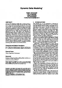
1.1 Problem Statement Programming is an activity very prone to human error. As more and more features are implemented in a software system by different programmers, progress will often slow to a crawl. It is all too easy for programmers to lose overview of what their code is doing when it is spread across the code base surrounded by the code of others. This can result in bugs and inevitably much time will need to be spent on maintenance. This, in turn, results in more expensive software that takes longer to reach the user. To prevent a large software system from collapsing under its own complexity, its code needs to be well-structured. Manny Lehman (remembered as the Father of Software Evolution) stated the following as his second law of software evolution [48, 119]: “As a program is evolved its complexity increases unless work is done to maintain or reduce it.” Ideally we want all code related to a certain feature (sometimes called concern) to be grouped together in one module —which is called feature modularity or feature locality [89, 109, 156]— and code belonging to different features not to be mixed together — which is called separation of concerns [96, 112, 114, 147]. But many concerns cannot be easily captured by existing abstractions. They are known as cross-cutting concerns. By their very nature their implementation needs to be spread around the code base, so modularization and separation of concerns are still elusive. The software engineering discipline that has the most to gain from those properties is Software Product Line Engineering (SPLE), a relatively new development. To quote van der Linden, Schmid and Rommes [122]: “Software product lines represent perhaps the most exciting paradigm shift in software development since the advent of high-level programming languages.” SPLE is concerned with the development and maintenance of multiple software systems at the same time, each possessing a different (but often overlapping) set of features — a form of mass customization [117, 155].1 This gives rise to an additional need. It is no longer enough that the code for a given feature is separated and modular; it also need to be composable and able to deal gracefully with the presence or absence of other features. We need to be able to make a selection from a set of available features and have the corresponding software mechanically generated for us — a process known as automated product derivation [1, 2, 65, 163] (Figure 1.1). That is no small order.

1 The

term ‘product line’ is really a misnomer. It comes from 1834, when a typical retailer had only a small number of products, lined up in front of him [55, 157]. In a (software) product line, neither the products nor the features need to be linearly ordered in any way. The term ‘product family’, used primarily in Europe [155], is therefore technically more accurate. Nonetheless, ‘product line’ is used much more widely, so we’ll stick with it.

1.2. EXISTING APPROACHES

5 Code Base

.Feature Selection

Automated Product Derivation

Software Product

Figure 1.1: The process of Automated Product Derivation.

1.2 Existing Approaches A number of programming paradigms have recently emerged out of a need to solve the problem of cross-cutting concerns. Among the more recent are Aspect Oriented Programming (AOP) and Feature Oriented Software Development (FOSD) [13, 104, 110, 125, 156]. We now summarize these existing approaches.

1.2.1 Aspect Oriented Programming Around the turn of the millenium, Aspect Oriented Programming (AOP) [107, 112, 114, 126, 133, 144] was proposed to tackle cross-cutting concerns. An aspect can specify code (called advice) to be added at specific locations (called pointcuts) in an existing code base. All code belonging to a concern can be grouped together. AOP is a step in the right direction, as many related code fragments that once had to be spread around can now be grouped into one aspect. Generally, however, AOP only supports the insertion of statements around identified join-points inside methods and the addition of members to an existing class (using inter-type declarations [12]). Moreover, there has been a general lack of support from AOP to help us reason about —and coordinate— the interaction between different concerns [51], though there has been recent work attempting to improve this situation [129].

1.2.2 Feature Oriented Software Development In literature, Feature Oriented Software Development (FOSD) is often equated with software product line engineering, so approaches that claim to follow FOSD are often capable of automated product derivation to some degree. A Software Product Line (SPL) is a collection of similar software systems (or software products) that differ only by which features they support and can, therefore, share a lot of the same source code. FOSD and SPLE share basically the same techniques. Compared to AOP, these techniques have the added benefit of supporting automated product derivation. To accomplish this, methods were developed to express the variability between products: where and how can the code of one product differ from that of another, and which features account for those differences? Techniques for expressing SPL variability can be divided into two main categories [108]: annotative techniques and compositional techniques.

6


1.2.3 Annotative Software Product Line Techniques An annotative code-base consists of the totality of available code — all features included. Specific annotated parts of that code —parts belonging to features we don’t want— can be removed to create a final program [106, 108, 181]. Of all approaches to automate product derivation, the annotative approach is probably most popular one practice. A prominent example of this is the Linux kernel, which is an immense collection of C code annotated by #ifdef preprocessor directives, which allow conditional compilation [171]. But in the annotative approach, code is not gathered in modules; just annotated wherever it appears. Consequently, it does not enjoy the modularity or separation of concerns we want. Furthermore, it forces feature related code into an improper structure: a linear textual order. This is an overspecification, as it can never be clear whether the order between two different lines of code was by design, or forced upon the developers by the annotative paradigm. As the order between two statements can be semantically significant in an imperative programming model, this can cause unanticipated bugs and complexity in the long run.

1.2.4 Compositional Software Product Line Techniques Of particular interest to us are the so-called compositional techniques, such as GenVoca [30], AHEAD [31] and Delta Modeling [160, 162–164]. In contrast to the annotative techniques, the idea here is to gather all code belonging to a feature —or a closely related set of features— into a single module: a feature module. To obtain any specific product from the product line, one only has to choose the appropriate set of modules and apply them to the core product —the code that contains only the bare basics— in the proper order. When applied, they can then modify the core in order to integrate their features. This is generally done by a process known as invasive composition [23], called so because feature modules often need break object oriented encapsulation and class boundaries in order to apply the proper modifications to the code.

1.3 The Abstract Delta Modeling Approach This thesis is about Delta Modeling, a compositional technique for implementing variability of software product lines. Its feature modules are called deltas, as they describe the difference between two systems. Rather than focus merely on software, we define an abstract approach to delta modeling called Abstract Delta Modeling (ADM), which comprises a number of related formalisms. These allow us to reason about delta modeling without having to consider any specific programming paradigm. A great number of relevant concepts can be discussed without ever mentioning software. In fact, focussing on software too early —or worse, a specific programming language— could narrow our vision and cause us to miss good ideas. Dave Clarke, Ina Schaefer and myself [1, 2] first introduced ADM as a formal approach for modeling software product lines. These articles give an algebraic description of deltas and how they can be combined and linked to the higher level notion of feature. One of the main contributions of that work was a way of organizing deltas in a partially ordered structure. This allows us

1.4. A RUNNING EXAMPLE: THE EDITOR PRODUCT LINE

7

to express relations and dependencies between deltas that closely mirror the original design intentions. Specifically, we could now reason about conflicting deltas —independent deltas with incompatible implementations— and conflict resolving deltas — specialized modules to mediate conflicts and streamline feature interaction. Already in that work, delta modeling was not restricted to software, but rather product lines of any domain. So even though the main inspiration for ADM was to structure software systems, it can just as readily be used to formulate sets of mathematical equations, model possible hardware configurations or design a line of office furniture. Since the original article, delta modeling has been extended and refined in several directions [3–7], all of which we will discuss in this thesis. In particular, a modal logic was created to make it easier to reason about the semantics of products and deltas; a development workflow for product lines was introduced; and last but not least, an abstract semantics for dynamic delta modeling was developed, allowing deltas to be applied at runtime, on demand, based on environmental conditions. Much of this theory has already been put into practice. Delta modeling was implemented in the ABS modeling language [8, 52] (developed by the HATS project), and I have implemented it for Javascript and LATEX. The development workflow was applied to the Fredhopper Access Server [7] —an industrial scale case study—, and I applied dynamic delta modeling techniques to the development of a profile management application for Android.

1.4 A Running Example: The Editor Product Line In this section we introduce the plans for a fictional software product line of source code editors such as you might find in IntelliJ IDEA [99] or Eclipse [139]. We will use this product line as an illustrative example throughout most of the thesis. Section 1.4.1 describes the features we want to implement and Section 1.4.2 gives an idea of how our delta modeling based implementation will work.

1.4.1 The Specification The specification of the Editor product line includes a set of feature configurations corresponding to the different kinds of editors we want to be able to generate. Each represents a different selection of features to include in the final product. Such a set of feature configurations is called a feature model. Figure 1.2 shows a feature diagram [66] representing the feature model of the Editor product line. We’ll consider the following features: • Editor (𝐸𝑑) is the only mandatory feature of the product line. It represents basic text editing functionality. • Printing (𝑃𝑟) allows the user to print the code in the editor on paper. • Syntax Highlighting (𝑆𝐻) displays code in color for easier recognition of different programming language constructs. • Error Checking (𝐸𝐶) performs simple grammatical analysis on code and underlines certain errors. Hovering over an error with the mouse-pointer triggers a tooltip with extra information.

8


Editor

. Printing

Syntax Highlighting

Error Checking

Tooltip Info

Semantic Analysis Figure 1.2: The feature diagram of the Editor product line. Each box . represents a feature. The base feature (Editor) is mandatory. A connector with an open circle at the end . indicates an optional subfeature. A subfeature can only be selected if its parent feature is also selected. A curve between two . connectors indicates a mutually exclusive choice between subfeatures.

• Error Checking has an optional subfeature: Semantic Analysis (𝑆𝐴). It performs more sophisticated error analysis of program code. • Tooltip Information (𝑇𝐼) shows contextual information in a tooltip when the mouse-pointer hovers over some code. Since Error Checking can also trigger tooltips, we decide to make the two features mutually exclusive, i.e., a final product should not include both. This product line consists of 16 different editors, as there are 16 possible feature configurations.

1.4.2 An Implementation using Deltas We now look at a delta-based implementation of the Editor product line in some object oriented programming language. It will be complete enough to generate all 16 possible end products, yet modular enough not to require any code duplication. Figure 1.3 shows an overview of the entire code-base. Each delta is represented by a dashed box, displaying the modifications it can perform to the program. The internal boxes mimic UML class-notation [159]. The keywords add, mod and rep respectively indicate addition, modification and replacement of code artefacts. A modification descends one level to apply more fine-grained transformations. Each delta is also annotated with its application condition, indicating the feature configurations for which it should be applied. The Editor code-base consists entirely of deltas. They are designed to incrementally modify the empty program (which is not shown). Each feature 𝑓 is implemented by a single delta — which we’ll call 𝑑𝑓 . For example, 𝑑𝐸𝑑 implements the basic editing functionality of 𝐸𝑑 by adding the Editor class to the empty program. It is always applied, because 𝐸𝑑 is a mandatory feature.

1.4. A RUNNING EXAMPLE: THE EDITOR PRODUCT LINE

add Editor m_model: Model;

.

.

9

.

mod Editor

init(m: Model): void model(): Model font(c: int): Font onMouseOver(c: int): void

rep onMouseOver(c: int): void 𝑇𝐼 𝐸𝑑

.

.

.

mod Editor add m_printer: Printer

mod Editor add m_syntaxhl: SyntaxHL;

mod Editor add m_errorch: ErrorCh;

mod init(m: Model): void add print(): void

mod init(m: Model): void rep font(c: int): Font

mod init(m: Model): void rep font(c: int): Font rep onMouseOver(c: int): void

add SyntaxHL m_model: Model;

add ErrorCh m_model: Model;

init(m: Model): void color(c: int): Color

init(m: Model): void errorOn(c: int): bool errorText(c: int): string

.

𝑃𝑟

. ..

.

𝑆𝐻

𝐸𝐶

.

.

mod Editor

.

mod Editor

rep print(): void

mod ErrorCh

rep font(c: int): Font 𝑃𝑟 ∧ 𝑆𝐻

𝑆𝐻 ∧ 𝐸𝐶

mod add rep rep

init(m: Model): void process(m: Model): void errorOn(c: int): bool errorText(c: int): string 𝑆𝐴

Figure 1.3: A delta diagram of the Editor product line implementation. Each dashed . box represents a delta with an overview of the modifications it can apply to the core product in a UML-like notation. Method bodies are omitted for brevity. The arrows . indicate which deltas are allowed to overwrite or alter the modifications of others. The propositional logic formula . attached to the bottom right corner of each delta represents the feature configurations for which that delta should be applied.

The other deltas add some functionality on top of the basic editor, just as a programmer would in traditional software engineering. For instance, 𝑑𝑃𝑟 implements the 𝑃𝑟 feature by making some modifications to the Editor class. It adds a field m_printer, a method print() and it modifies the pre-existing init() method. Since 𝑑𝑃𝑟 continues where 𝑑𝐸𝑑 left off, it is important that they are applied in the right order. That’s where the arrows in the diagram come in. They represent the partial application order, a part of the code-base design. Because of this order, 𝑑𝑃𝑟 can be written with the certainty that 𝑑𝐸𝑑 will be applied first. This is always necessary for deltas that implement subfeatures. Besides the subfeatures on the first level, it is also the case for 𝑑𝑆𝐴 , which implements the second-level subfeature 𝑆𝐴. By not placing an order between two deltas, a developer indicates that the order in which the deltas are applied should not matter — an important design intention.

10


This makes the code-base very robust to change, as code dependencies are made explicit in the design. If the code of 𝑑𝐸𝑑 is ever changed, the developers of 𝑃𝑟 may receive an automated warning, so they can determine whether they should make corresponding changes to 𝑑𝑃𝑟 . In certain situations the application order can even ensure an automated error message when two independent deltas make incompatible changes to the program. For example, because of the limited interface of Editor, 𝑑𝑆𝐻 and 𝑑𝐸𝐶 both need to replace the font(int) method; the former to change the color of the content, the latter to underline it in case of errors. (Incidentally, note that besides modifying Editor, both deltas also add a new class of their own.) Since neither delta has priority over the other —and rightfully so— there is a conflict in the code-base that needs to be resolved, and it can be automatically detected. We resolve the conflict with what we call a conflict resolving delta. The delta annotated with 𝑆𝐻 ∧ 𝐸𝐶 —which we’ll call 𝑑𝑆𝐻∧𝐸𝐶 — is applied only in situations where this conflict would occur and replaces the font(int) method with a final version that properly combines the implementations of 𝑑𝑆𝐻 and 𝑑𝐸𝐶 . At first glance it appears as though 𝑑𝐸𝐶 and 𝑑𝑇𝐼 are also in conflict, as they both replace the onMouseOver(int) method. However, this will never be a problem. By the feature model (Figure 1.2) the features 𝐸𝐶 and 𝑇𝐼 can never be selected together, so there can never be a conflict in the first place. So what is 𝑑𝑃𝑟∧𝑆𝐻 doing? 𝑑𝑃𝑟 and 𝑑𝑆𝐻 are not in conflict. However, we’d like these two features to be more than the sum of their parts. When we can both highlight the code and print it, it makes sense that we should also be able to print the code in color. We call 𝑑𝑃𝑟∧𝑆𝐻 an interaction implementation delta. It replaces print() with a version that makes use of the font(int) method from 𝑑𝑆𝐻 . It is similar in many ways to a conflict resolving delta, but the reason we need it cannot be detected automatically. And so we have an implementation that explicitly links features to their corresponding code. It is modular: all code belonging to the same feature (combination) is grouped together in a delta. It has separation of concerns: code belonging to different features is separated. We also have automated product derivation: given any desired feature configuration, we can select the relevant deltas from the model, then apply them in the proper order. This description did leave out a lot of details. We will spend the rest of this thesis exploring those details.

1.5 Papers & Chapters This section outlines the chapter structure of this thesis and lists the publications on which it is based.

1.5.1 My Publications In October 2009 I presented my idea for conflict resolving deltas at a HATS working meeting in Leuven, Belgium. This began my collaboration with Dave Clarke and Ina Schaefer on Abstract Delta Modeling. I was fortunate to stumble upon a viable research idea so early on. It provided me with a sense of focus

1.5. PAPERS & CHAPTERS

11

for more than three years, improving and extending ADM. All of my publications since the abovementioned collaboration, therefore, are on the same topic, allowing for a thesis with a coherent narrative. A bibliography-style list of those publications can be found on Page 234. They are split off from the main bibliography, and are numbered sequentially throughout the thesis: [1–10] [1, 9] Abstract Delta Modeling This paper was written by Dave Clarke, Ina Schaefer and myself, and forms the theoretical core of this entire thesis. A technical report [9] accompanied the main paper [1], containing full proofs that did not fit within the page limit. I presented the paper at GPCE 2010 in Eindhoven, the Netherlands. It introduces an abstract notion of products, of deltas that can transform products, partially ordered delta structures called delta models and delta-based product lines. This theory is treated in Chapters 2 to 4. This paper is also the source of the Editor Product Line example of Section 1.4. I’ve chosen to extend it for this thesis, since it seems to have done a great job in helping fellow researchers understand the practical application of the theory. It is simple and familiar, yet flexible enough to demonstrate most of ADM’s benefits. [5] Delta Modeling Workflow This paper was written by me in 2011 and presented at VaMoS 2012 in Leipzig, Germany, together with its companion paper [7]. ADM is meant to model real-world software product lines, but the main work only presented a formal framework; one that encompasses a vast expressive space, but without any guidelines to its recommended use. So this paper proposed a development workflow based on ADM, which allows concurrent and isolated development of features while preserving beneficial global properties. The workflow is treated in Chapter 7, and a more thorough formalization can be found in Appendix A. [7] Delta Modeling in Practice, a Fredhopper Case Study This paper was written by Radu Muschevici, Peter Wong and myself in 2011, and put the Delta Modeling Workflow through its paces on the industrial-scale case study of the Fredhopper Access Server. I presented it at VaMoS 2012 together with the theoretical paper described above. It includes an analysis on the effectiveness of the workflow in a practical setting, which is included in Chapter 7. [3] A Modal Logic for Abstract Delta Modeling This paper was written by Frank de Boer, Joost Winter and myself, one of three publications presented by me at SPLC 2012 in Salvador, Brazil. It presents a multimodal logic meant for reasoning about the effects of deltas and the semantics of products. Its main innovation is a modality for delta models. This theory is treated fully in Chapter 6. This was the first paper to interpret deltas as mathematical relations between products, rather than functions. This idea has been fully integrated into the main ADM theory of this thesis — something which has not yet been published. It’s had a particularly profound effect on Chapters 2 and 3.

12


[6] Dynamic Delta Modeling This paper was written by me and presented at SPLC 2012 in Salvador, Brazil. It put the flexibility of ADM to the test, as it applies the formalism in a dynamic setting: the selected feature configuration can change at runtime, and the system has to adapt in real time. The main case-study is an Android application which allows automated profile management, reconfiguring a mobile device’s operating profile based on environmental factors. This paper is covered fully in Chapter 8, together with its submitted extension [⌛1]. [4] Abstract Delta Modeling: My Research Plan This is a PhD research plan submitted to the doctoral symposium colocated with SPLC 2012. It describes my plans for this thesis and was published in the digital proceedings of the conference. The thesis does not fulfill all of my earlier predictions, but I believe that in most of those instances, the result was a better reading experience. [2] Abstract Delta Modeling (Journal Version) This paper was written by Dave Clarke, Ina Schaefer and myself as an extended version of the ADM conference paper [1, 9], accepted to a special issue of MSCS. (We received notification of acceptance a long time ago, but the article has not yet been published as of this writing, because of a backlog.) This article subsumes the original work. Aside from a more detailed treatment of the formalism, its main addition was that of nested delta models, which are discussed in Sections 3.6 and 4.5. [8] HATS Abstract Behavioral Specification: The Architectural View This paper was written by Reiner Hähnle, Einar Broch Johnsen, Michael Lienhardt, Davide Sangiorgi, Ina Schaefer, Peter Y. H. Wong and myself and submitted as a HATS publication, published by Springer in 2013. It describes the Abstract Behavioral Specification (ABS) language from an architectural perspective, a perspective that includes delta modeling. My contribution to this article was an accounting of the Delta Modeling Workflow tailored to ABS, which is summarized in Chapter 7. [10] The pkgloader and lt3graph Packages: Toward simple and powerful package management for LaTeX I was invited to write this article by the editor of TUGboat, the Communications of the TEX Users Group, based on my work on the pkgloader LATEX package. This package oversees the package loading process and uses delta modeling principles to address one of the major frustrations of LATEX: package conflicts. The article introduces the pkgloader package, as well as lt3graph, a LATEX3 library used by pkgloader to do most of the heavy lifting. This practical application of delta modeling is treated in Chapter 5.

1.5.2 Unpublished Work The following have been written, but not yet accepted for publication.


13

[⌛1] An Operational Semantics for Dynamic Product Lines This paper was written by me in 2013, and submitted to a SoSyM Special Issue on Integrated Formal Methods. It is loosely based on the first paper on dynamic delta modeling [6]. It takes a more formal, more general approach and subsumes the earlier work. The main new contribution is an operational semantics, which now formalizes the previously vague notion of ‘strategy’. The new approach incorporates unrestricted feature models as well as relational deltas, whereas the original work required that the feature model considers all features to be independent and all deltas to have a functional behavior. Finally, the description of the case-study has been greatly extended. It is on this article that Chapter 8 is based.

[⌛2] A Formal Software Product Line Development Workflow This paper was written by me in 2013, but has not yet been submitted. It extends the first abstract paper on the Delta Modeling Workflow [5], and subsumes most of the theory from that paper. The main contribution absent from the earlier work is a focus on concurrent development and a proof that such concurrent development is possible without sacrificing correctness. To that end, an operational semantics is used to model the various implementation steps of the workflow. This theory is presented in Appendix A.

1.5.3 The Chapters The distribution of the work over the chapters of the thesis is based on narrative merit, rather than a one-to-one correspondance. Pretty much every publication has influenced every chapter in some way, but there are some clear connections, which are mentioned in the summaries below.

Chapter 1: Introduction What remains of the current chapter is a set of typographic conventions in Section 1.6 —recommended, if you plan on reading a significant portion of the other chapters— and some preliminary theory on discrete mathematics in Section 1.7, which is meant primarily as a reference.

Chapter 2: Algebraic Delta Modeling This chapter introduces the basic building blocks of delta modeling: products and deltas, as well as their characteristics and interactions. Most of the theory comes from the original papers [1, 2], but it adopts refinements introduced in other papers. Notably, it introduces the semantics of deltas as relational, rather than functional, which was first done in the papers on delta logic [3] and dynamic delta modeling [6]. It also contains some unpublished material. In particular, a number of new algebraic interpretations are discussed in Section 2.6.

14


Chapter 1 . Introduction

Chapter 2 Algebraic Delta Modeling

Chapter 3 Delta Models

Chapter 4 Product Lines .

.

Chapter 5 LATEX Meets Delta Modeling

Chapter 6 Delta Logic

.

.

Chapter 7 Delta Modeling Workflow

Chapter 8 Dynamic Product Lines

Chapter 9 Conclusion Figure 1.4: The suggested reading order of the thesis. Chapters 5 to 8 can basically be read in any order. Before that, however, each chapter builds upon the theory of its predecessor.


15

Chapter 3: Delta Models This chapter introduces the partially ordered structure and conflict resolution models that first inspired the work on ADM. Again, most of this comes from the original ADM papers [1, 2], but includes adaptation to the relational semantic view. The chapter also introduces a distinction between several different types of delta model semantics, one of which —conjunctive semantics— is as of yet unpublished. Chapter 4: Product Lines This chapter introduces features and ADM-based product lines and is the final chapter based on the original work [1, 2]. The theory in this chapter has been influenced most by the work on the development workflow [5], which split up the description of a delta-based product line into a specification and an implementation, and introduced the concept of parametric deltas: deltas that behave differently for different feature configurations. Chapter 5: LATEX Meets Delta Modeling This chapter demonstrates the LATEX implementation of delta modeling by documenting two new LATEX-packages. The delta-modules package defines deltas that can be used for the preparation of documents, and families of related documents. For example, this thesis was prepared using the delta-modules package, and different versions of the thesis are available that skip certain topics for a different reading experience. The pkgloader package solves a long-existing problem with the LATEX ecosystem: that of package management. Many document authors suffer from the fact that various LATEX packages are mutually incompatible, and the fact that this is very poorly documented. The pkgloader package uses delta modeling principles to load third party packages in the proper order, apply code to resolve certain package conflicts or, as a last resort, provide the user with a clear error message. Chapter 6: Delta Logic This chapter introduces a modal logic for reasoning about products and deltas. It is almost fully based on [3], but some theory was already introduced in earlier chapters. It presents a multi-modal language and a number of proof techniques with accompanying soundness and completeness proofs. A possible new adaptation to hybrid logics is briefly discussed as well. Chapter 7: Delta Modeling Workflow This chapter introduces a recommended workflow for building delta-based product lines. It is almost fully based on the corresponding publications [5, 7, 8]. The theory is strengthened by a new formulation in terms of operational semantics based on an as of yet unpublished paper [⌛2]. To improve readability, the operational semantics is not exposed in the chapter itself, but is instead presented in Appendix A.

16


Chapter 8: Dynamic Product Lines This chapter introduces dynamic delta modeling: a basis for modeling product lines that can adapt at runtime to a dynamically changing feature configuration. It is based on the corresponding paper [6], though thoroughly reworked and extended since 2012. The new theory, based on an interplay between operational semantics and Mealy machines, has been submitted to a SoSyM special issue on integrated formal methods [⌛1]. Chapter 9: Conclusion This chapter summarizes the main contributions, goals and lessons of each chapter, and then presents a number of possible directions for future work.

1.6 Typographic Conventions This section contains the various typographic conventions used throughout this thesis. Knowing them is not necessary for understanding the theory, but it can help the reader to spot certain constructs at a glance and to read and parse the text more efficiently.

1.6.1 Fonts The following variations in font serve a special purpose: • A Serif Roman typeface, apart from being used for the prose, is also used for the names of mathematical functions. • Italic type is used to put emphasis on certain words or phrases, either in a linguistic sense (“we can represent product lines of any domain”) or to mark certain notions as important to the theory (“units called deltas”). It is also used for the names of mathematical variables and constants. • A Sans Serif typeface is used for the names of mathematical predicates, relations and classes. • 𝒞𝑎𝑙𝑖𝑔𝑟𝑎𝑝ℎ𝑖𝑐 or 𝔉𝔯𝔞𝔨𝔱𝔲𝔯 typefaces are used in mathematical formulas for specific kinds of variables related to the theory of discourse, usually to maintain consistency with previous work. • A Monospaced typeface is used for (fragments of) source-code. Inside source code, keywords and core language constructs are bold, values are italic, comments are /*gray*/ and types are green. The color contrast should still be high enough for the last two to be readable (though not distinguishable) when printed in grayscale. • Small caps is used in Chapter 8 and Appendix A for the names of specific inference rules in the operational semantics. The definition of new inference rules sets the pace of the respective chapters and their names form convenient reference points.

1.6.2 Formal Concepts The main chapters of this thesis present various theories. The definitions, assumptions and results that constitute the formalisms for those theories are placed in clearly delimited blocks that break up the running text. These concepts are numbered sequentially per chapter, and they come in the following flavors:

1.6. TYPOGRAPHIC CONVENTIONS

17

0.1. Definition: a formal definition

⌟

0.2. Notation: a formal notation

⌟

0.3. Action: a formal action that may be taken by a developer

⌟

0.4. Example: an example of a formal concept

⌟

0.5. Axiom: a formal restriction on an existing definition

⌟

0.6. Theorem: an important formal result

◻

▹ 0.7. Lemma: an intermediate or smaller formal result

◻

▸. 0.8. Corollary: a formal result that readily follows from a previous result

◻

.In the left margin of each of these types of blocks you may find one of two symbols. A white triangle ( ▹) indicates that the concept belongs to one of the concrete examples or case studies of the thesis, .rather than the overall abstract formalism. A black triangle ( ▸) indicates concepts of a greater scope. Blocks without either symbol are local in nature and could be skipped without missing too much in the long run. But a black triangle indicates that later sections or chapters will refer back to the concept in question. Not all formal results will be accompanied by a proof. A lot of the required proofs are conceptually quite simple, but long, tedious and generally uninteresting to read. A proof is included only if reading it would provide valuable insight into the theory. For some results about the running example, a mechanically checked proof has been written with the Coq proof assistant [36]. Those results show the Coq logo ( ) .in the right margin. This gives the reader some confidence in the result without requiring them to plow through quadruply nested case distinctions. .

1.6.3 PDF Features When viewing the PDF file of this thesis on a computer monitor, you have access to several extra features. First, there are clickable hyperlinks between sections, formal environments, bibliography references and more. Second, the logo next to the results checked with the Coq proof assistant can be clicked to download an embedded copy of the Coq proofs. This will only work for certain PDF viewers, such as Adobe Reader.

.

18


1.7 Mathematical Preliminaries This section establishes the basic mathematical notations and definitions that are used in this thesis. We assume that the reader already has an intuitive grasp of the concepts in this section, as the treatment will be dense. A basic grounding in the topics of Sections 1.7.1 to 1.7.7 can be gained from any introductory textbook on discrete mathematics [123]. As for the more specialized material of Sections 1.7.8, 1.7.9, 1.7.10 and 1.7.11, there are some great introductions on abstract algebra [179], modal logic [42] and operational semantics [153] to be found. I found these cited sources well written and accessible.

1.7.1 Sets A set is an unordered collection of elements —finite or infinite— which does not contain the same element more than once. For this thesis, an understanding of naive set theory [83] is sufficient. ▸ 1.1. Definition (Basic Set Concepts): The basic set notations are as follows, for any set 𝑆, elements 𝑒, 𝑒1 , …, 𝑒𝑛 , predicate 𝖯, relation 𝖱 and function f: { 𝑒1 , …, 𝑒𝑛 } { f(𝑒) | 𝖯(𝑒) } { 𝑒 𝖱 𝑔 | 𝖯(𝑒) } 𝑒∈𝑆 |𝑆|

the finite set containing only the elements 𝑒1 , …, 𝑒𝑛 the set of all elements f(𝑒) such that 𝑒 satisfies 𝖯 an abbreviation for { 𝑒 | 𝑒 𝖱 𝑔 ∧ 𝖯(𝑒) } 𝑒 is a member of 𝑆 the cardinality of 𝑆

The following relations and operations are defined for all sets 𝑆, 𝑇 : 𝑆⊆𝑇 𝑆⊂𝑇 𝑆∪𝑇 𝑆∩𝑇

⟺ ≝ ⟺ ≝ ≝ ≝

∀𝑒 ∈ 𝑆: 𝑒 ∈ 𝑇 𝑆⊆𝑇 ∧ 𝑆≠𝑇 {𝑒 | 𝑒 ∈ 𝑆 ∨ 𝑒 ∈ 𝑇 } {𝑒 | 𝑒 ∈ 𝑆 ∧ 𝑒 ∈ 𝑇 }

𝑆∖𝑇 𝑆⊖𝑇 Pow(𝑆) 𝑆∁

≝ ≝ ≝ ≝

{𝑒 ∈ 𝑆 | 𝑒 ∉ 𝑇 } (𝑆 ∪ 𝑇 ) ∖ (𝑆 ∩ 𝑇 ) { 𝑆′ ∣ 𝑆′ ⊆ 𝑆 } 𝑈 ∖𝑆

A universal set 𝑈 is assumed to be clear from context when the 𝑆 ∁ notation is ⌟ used. ▸ 1.2. Definition (𝒏-ary Set Operations): The 𝑛-ary set operations ⋃ and ⋂ are defined as follows, for all sets 𝑆, properties 𝖯 and functions f: ⋃𝑆

≝

{ 𝑒 | ∃𝑠 ∈ 𝑆: 𝑒 ∈ 𝑠 }

⋃𝖯(𝑔) f(𝑔)

≝

⋃ { f(𝑔) | 𝖯(𝑔) }

⋂𝑆

≝

{ 𝑒 | ∀𝑠 ∈ 𝑆: 𝑒 ∈ 𝑠 }

⋂𝖯(𝑔) f(𝑔)

≝

⋂ { f(𝑔) | 𝖯(𝑔) }

where 𝑔 is a fresh variable name.

⌟

1.7. MATHEMATICAL PRELIMINARIES

19

▸ 1.3. Notation (Important Sets): The following specific sets are used often: ∅ ℕ+ ℕ ℤ ℝ

the the the the the

empty set positive natural numbers 1, 2, 3, … natural numbers 0, 1, 2, … integers …, −2, −1, 0, 1, 2, … real numbers

Each is a strict subset of the ones that follow.

⌟

1.7.2 Tuples To represent ordered collections of elements, we use tuples. ▸ 1.4. Notation (Tuples): A tuple can be given directly as a comma-separated list of elements between parentheses (𝑒, 𝑔, ℎ), or sometimes angle brackets ⟨𝑒, 𝑔, ℎ⟩. ⌟ The order between the elements is significant. Tuples with 2, 3, 4, 5 and 𝑛 elements are respectively called pairs, triples, quadruples, quintuples and 𝑛-tuples. ▸ 1.5. Definition (Cartesian Product): The Cartesian product operation × on two sets 𝑆, 𝑇 is a set of pairs defined as follows: 𝑆×𝑇

≝

{ (𝑒, 𝑔) | 𝑒 ∈ 𝑆 ∧ 𝑔 ∈ 𝑇 }

⌟

▸ 1.6. Definition (𝒏-ary Cartesian Product): For some number 𝑛 ∈ ℕ+ , the 𝑛ary Cartesian product on sets 𝑆1 , …, 𝑆𝑛 is a set of 𝑛-tuples defined as follows: 𝑆1 × ⋯ × 𝑆 𝑛

≝

{ (𝑒1 , …, 𝑒𝑛 ) | 𝑒1 ∈ 𝑆1 ∧ ⋯ ∧ 𝑒𝑛 ∈ 𝑆𝑛 }

⌟

▸ 1.7. Definition (Cartesian Power): For any number 𝑛 ∈ ℕ+ , the 𝑛th Cartesian power of a set 𝑆 is defined as follows: 𝑆𝑛

≝

𝑆 ×⋯×𝑆 ⏟⏟⏟⏟⏟⏟⏟

⌟

𝑛

1.7.3 Sequences Sequences are basically tuples, but always contain elements of the same type and are usually of unspecified (but finite) length. ▸ 1.8. Definition (Sequences): Given a set 𝑆, the set of all finite sequences of elements from 𝑆 is defined as follows: 𝑆∗

≝

⋃ 𝑆𝑛

⌟

𝑛∈ℕ

▸ 1.9. Definition (Sequence Concatenation): The concatenation of two sequences 𝑒 = (𝑒1 , …, 𝑒𝑛 ) and 𝑔 = (𝑔1 , …, 𝑔𝑚 ) with 𝑛, 𝑚 ∈ ℕ is defined as follows: 𝑒

⌢

𝑔

≝

(𝑒1 , …, 𝑒𝑛 , 𝑔1 , …, 𝑔𝑚 )

A sequence on either side with only one element may be abbreviated by omitting ⌟ the parentheses, e.g., 𝑒 ⌢ (𝑔1 , 𝑔2 ) instead of (𝑒) ⌢ (𝑔1 , 𝑔2 ).

20


1.7.4 Relations ▸ 1.10. Definition (Relation): Given 𝑛 ∈ ℕ+ , an 𝑛-ary relation 𝖱 over the sets 𝑆1 , …, 𝑆𝑛 is a subset of their Cartesian product: 𝖱 ⊆ 𝑆1 × ⋯ × 𝑆𝑛 . A unary ⌟ relation is also called a predicate.

▸ 1.11. Definition (Relation Operations): Given two binary relations 𝖱 ⊆ 𝑆 × 𝑇 and 𝖰 ⊆ 𝑇 × 𝑈 we define the following operations: 𝖰∘𝖱 𝖱−1 id𝑆

≝ ≝ ≝

{ (𝑒, ℎ) | ∃𝑔 ∈ 𝑇 : (𝑒, 𝑔) ∈ 𝖱 ∧ (𝑔, ℎ) ∈ 𝖰 } { (𝑔, 𝑒) | (𝑒, 𝑔) ∈ 𝖱 } { (𝑒, 𝑒) | 𝑒 ∈ 𝑆 }

with 𝖰 ∘ 𝖱 ⊆ 𝑆 × 𝑈 and 𝖱−1 ⊆ 𝑇 × 𝑆 and id𝑆 ⊆ 𝑆 2 . Note that relation ⌟ composition ∘ should be read from right to left.

▸ 1.12. Notation: For all sets 𝑆, 𝑆 ′ , elements 𝑒, 𝑔, ℎ ∈ 𝑆 and predicates 𝖯 ⊆ 𝑆: 𝖯(𝑒)

⟺ ≝

𝑒∈𝖯

𝖯(𝑆 ′ )

⟺ ≝

𝑆′ ⊆ 𝖯

Additionally, for all binary relations 𝖱, 𝖰 ⊆ 𝑆 × 𝑇 : 𝑒𝖱𝑔 /𝑔 𝑒𝖱 𝑒𝖱𝑔 𝑒𝖱𝑔𝖰ℎ 𝑒, 𝑔 𝖱 ℎ

⟺ ≝ ⟺ ≝ ⟺ ≝ ⟺ ≝ ⟺ ≝

(𝑒, 𝑔) ∈ 𝖱 ¬(𝑒 𝖱 𝑔) 𝑔𝖱𝑒 𝑒𝖱𝑔 ∧ 𝑔𝖰ℎ 𝑒𝖱ℎ ∧ 𝑔𝖱ℎ

𝖱(𝑒) 𝖱(𝑆 ′ ) img(𝖱) pre(𝖱) / 𝑒𝖱

≝ ≝ ≝ ≝ ⟺ ≝

{𝑔 | 𝑒 𝖱 𝑔} ⋃𝑒∈𝑆′ 𝖱(𝑒) 𝖱(𝑆) 𝖱 −1 (𝑆) 𝖱(𝑒) = ∅

𝖱(𝑒) is called the image of 𝑒 in 𝖱 and 𝖱−1 (𝑔) is called the preimage of 𝑔 in 𝖱. img(𝖱) and pre(𝖱) are called the image and preimage of the relation 𝖱 itself. / and 𝖱 often hold in literature, but The notational conventions regarding 𝖱 are not often formalized. In this thesis they always hold; as does the implied convention that binary relation symbols with a horizontal symmetry, such as ⌟ =, ≡ and ⇔, are also symmetric in a relational sense (Definition 1.13).

▸ 1.13. Definition (Binary Relation Properties): A binary relation 𝖱 ⊆ 𝑆 × 𝑇 may have the following named properties:

1.7. MATHEMATICAL PRELIMINARIES

𝑒

21

. ℎ

𝑔 𝖱

𝑆

𝑇

Figure 1.5: The visualization of a specific relation 𝖱 ⊆ 𝑆 × 𝑇 . The two groups of nodes represent the domain 𝑆 and codomain 𝑇 of the relation with 𝑒, 𝑔 ∈ 𝑆 and ℎ ∈ 𝑇 . The arrows represent the relation 𝖱 itself. They show, for example, / ℎ. that 𝑒 𝖱 ℎ and that 𝑔 𝖱 uniquely defined: fully defined: well defined: injective: surjective: bijective: one-to-one:

∀𝑒, 𝑔, ℎ ∈ 𝑆:

∀𝑒, 𝑔, ℎ ∈ 𝑆:

𝑒𝖱𝑔 ∧ 𝑒𝖱ℎ ⇒ 𝑔=ℎ pre(𝖱) = 𝑆 uniquely and fully defined 𝑒𝖱ℎ ∧ 𝑔𝖱ℎ ⇒ 𝑒=𝑔 img(𝖱) = 𝑇 surjective and injective uniquely defined and injective

Uniquely defined and fully defined are often called ‘functional’ and ‘total’. In the case that 𝑆 = 𝑇 we also distinguish the following: reflexive: symmetric: transitive: irreflexive: antisymmetric: asymmetric: total: discrete:

∀𝑒 ∈ 𝑆: ∀𝑒, 𝑔 ∈ 𝑆: ∀𝑒, 𝑔, ℎ ∈ 𝑆: ∀𝑒 ∈ 𝑆: ∀𝑒, 𝑔 ∈ 𝑆: ∀𝑒, 𝑔 ∈ 𝑆: ∀𝑒, 𝑔 ∈ 𝑆: ∀𝑒, 𝑔 ∈ 𝑆:

𝑒𝖱𝑒 𝑒𝖱𝑔 𝑒𝖱𝑔 /𝑒 𝑒𝖱 𝑒𝖱𝑔 𝑒𝖱𝑔 𝑒𝖱𝑔 /𝑔 𝑒𝖱

⇒ 𝑒𝖱𝑔 ∧ 𝑔𝖱ℎ ⇒ 𝑒𝖱ℎ ∧ 𝑒𝖱𝑔 ⇒ 𝑒=𝑔 /𝑔 ⇒ 𝑒𝖱 ∨ 𝑒𝖱𝑔 /𝑔 ∧ 𝑒𝖱

⌟

▸ 1.14. Definition (Transitive Closure): Given a binary relation 𝖱 ⊆ 𝑆 × 𝑆, define its transitive closure 𝖱+ ⊆ 𝑆 × 𝑆 and reflexive transitive closure 𝖱∗ ⊆ 𝑆 × 𝑆 as follows for all elements 𝑒, 𝑔 ∈ 𝑆: 𝑒 𝖱+ 𝑔

⟺ ≝

𝑒 𝖱 𝑔 ∨ ∃ℎ ∈ 𝑆: 𝑒 𝖱 ℎ 𝖱+ 𝑔

𝑒 𝖱∗ 𝑔

⟺ ≝

𝑒 = 𝑔 ∨ 𝑒 𝖱+ 𝑔

⌟

▸ 1.15. Notation (Inference Rule): A specific relation or set of relations is sometimes defined as the smallest relation(s) satisfying a particular set of inference rules. An inference rule consists of a conclusion and a set of premises, separated by a horizontal line: 𝑝𝑟𝑒𝑚𝑖𝑠𝑒 1 ⟩ ⟨𝑝𝑟𝑒𝑚𝑖𝑠𝑒 2 ⟩ … ⟨𝑐𝑜𝑛𝑐𝑙𝑢𝑠𝑖𝑜𝑛⟩ Free variables present in an inference rule can be consistently replaced by any ⌟ concrete value, i.e., they are under an implicit universal quantification. ⟨

22


Relations are important in this thesis, particularly because the semantics of deltas is expressed by relations. Relation diagrams such as the one in Figure 1.5 are occasionally used to illustrate relational concepts.

1.7.5 Functions ▸ 1.16. Definition (Function): A function from 𝑆 into 𝑇 is a well defined relation over the sets 𝑆, 𝑇 , which are respectively called its domain and codomain. 𝑆 → 𝑇 denotes the set of all functions from 𝑆 into 𝑇 . To declare a function f of that type, write f: 𝑆 → 𝑇 . When a function is declared this way, and we have (𝑒, 𝑔) ∈ f, we say that f(𝑒) = 𝑔. This overrides Notation 1.12 ( as we have ⌟ f(𝑒) ∈ 𝑇 rather than f(𝑒) ⊆ 𝑇 ). ▸ 1.17. Definition (Partial Function): A uniquely defined relation over 𝑆, 𝑇 that is not necessarily fully defined is called a partial function from 𝑆 into 𝑇 . The set of all partial functions from 𝑆 into 𝑇 is denoted 𝑆 ⇀ 𝑇 . To declare a partial function f of that type we write f: 𝑆 ⇀ 𝑇 . When 𝑒 ∉ pre(f) we say that f(𝑒) is undefined, or that f(𝑒) = ⊥ (assuming that ⊥ ∉ 𝑇 ). Otherwise, the ⌟ notation is the same as for functions. ▸ 1.18. Notation: A pair (𝑒, 𝑔) ∈ f in some partial function f, indicating that 𝑒 maps ⌟ to 𝑔, can also be denoted 𝑒 ↦ 𝑔. ▸ 1.19. Definition (Function Update): Given a function f: 𝑆 → 𝑇 and elements 𝑒 ∈ 𝑆 and 𝑔 ∈ 𝑇 , define the updated function f[𝑒 ↦ 𝑔] as follows, for all elements 𝑒′ ∈ 𝑆: 𝑔 if 𝑒 = 𝑒′ f[𝑒 ↦ 𝑔](𝑒′ ) ≝ { f(𝑒′ ) otherwise The same notation is defined for partial functions, in which case the update ⌟ f[𝑒 ↦ ⊥] is also available.

1.7.6 Transitive Relations ▸ 1.20. Definition (Preorder): A preorder is a transitive and reflexive relation.

⌟

▸ 1.21. Definition (Equivalence Relation): An equivalence relation is a transitive and symmetric relation (i.e., a symmetric preorder) denoted =, ≈, ≡, ⇔, … ⌟ ▸ 1.22. Definition (Orders): An order is a transitive and antisymmetric relation that is either: • reflexive, in which case it is called inclusive and denoted ≤, ≼, ⊆, ⊑, … • or irreflexive, in which case it is called strict and denoted void”, 𝑐𝑙 = ⎨ ⎬ “m_name = args[1]”, { ( ) } { } “output("Hello " + m_name)” ⎩ ⎭

32

CHAPTER 2. ALGEBRAIC DELTA MODELING

But from now on we’ll often use pseudo-code instead, and assume the abstract mathematical structure to be understood: 1 2 3 4 5 6 7

class { m_name: String; run(args: String[]) : void { m_name = args[1]; output("Hello " + m_name); } }

⌟

And finally, we define packages. A package can contain any number of classes mapped by name: ▸ 2.5. Definition (Packages): A package is a finite partial function 𝑝𝑘𝑔: ℐ𝒟 ⇀ 𝒞ℒ, ⌟ mapping identifiers to classes. The set of all packages is denoted 𝒫𝒦𝒢.

2.1.2 The DeltaEditor Package We now use this language to write a small package implementing a bare-bone version of the source code editor introduced in Section 1.4: ▹ 2.6. Example: The software product “DeltaEditor core”: 1 2 3

package DeltaEditor { class Editor { m_model: Model;

4

init(m : Model) : void { m_model = m; };

5 6 7 8

model() : Model { return m_model; };

9 10

font(c : int) : Font { Font result = new Font(); result.setColor(Color.BLACK); result.setBold(false); result.setUnderlined(false); return result; };

11 12 13 14 15 16 17 18

onMouseOver(c : int) : void { };

19

};

20 21

}; Assume that some other class (imported from a widget library perhaps) does most of the work, drawing and managing the visual interface. It is our job to implement the model(), font(int) and onMouseOver(int) methods so that the widget library has the necessary information to manage the editor.

2.1. INTRODUCTION

33

2.1.3 Implementing Syntax Highlighting Now, we implement some additional features in the traditional manner. This will demonstrate some of the disadvantages of the traditional approach —a lack of modularity, separation of concerns and variability control— and thereby motivate the work on delta modeling. The first feature is Syntax Highlighting, which changes the font of the content to provide a visual distinction between different language constructs. To accomplish this we develop a new class inside the DeltaEditor package to handle the business logic of parsing the model and determining the correct font for each individual character. We then add an instance of it to the Editor class, initialize it and, finally, replace the font(int) method with one that consults the new class. The resulting program looks as follows (the modified lines have been highlighted): ▹ 2.7. Example: The software product “DeltaEditor with 𝑆𝐻”: 1 2 3

.4

package DeltaEditor { class Editor { m_model : Model; m_syntaxhl : SyntaxHL;

5

init(m : Model) : void { m_model = m; m_syntaxhl = new SyntaxHL(m); };

6 7

.8 9 10


11 12

font(c : int) : Font { return m_syntaxhl.font(c); };

13 14 . 15 16

onMouseOver(c : int) : void { };

17

};

18 19 20 .

class SyntaxHL { m_model : Model;

21 . 22 . 23 .


24 . 25 .

font(c : int) : Font { /* something complicated */; };

26 . 27

}; };

Note that to implement this one feature, we were forced to make changes in four different places. When, in the future, another developer needs to change one of the highlighted code-fragments, they may well neglect to make corresponding changes to the other fragments, which is how bugs are introduced. Also, keep in mind that this is an oversimplified example. In a full application,

34


the implementation of a feature like this would involve designing toolbar buttons and configuration screens, developing code for user interaction and code to link models, views and controllers — not to mention the code necessary for proper interaction with other features. The point is, practically all software features are cross cutting concerns: their code needs to be spread around the code base to do its job properly, at least if we’re using programming models like OOP. This is a well-known problem in the world of software engineering. When software approaches certain levels of complexity, it becomes harder and harder to properly maintain it. We therefore strive towards the following goal: Goal: Find a way to ‘group together’ code related to the same feature. This is called feature modularity or feature locality [89, 109, 156].

2.1.4 Implementing Error Checking We now add another feature: Error Checking. We’d like certain syntactic errors to be underlined, and to show a tooltip when the mouse cursor hovers over them. Similar to before, a new class is responsible for the business logic, and several lines in the base class are added or modified to accomodate the new functionality. After implementing this feature, the resulting package might look as follows (again with the modified lines highlighted): ▹ 2.8. Example: The software product “DeltaEditor with 𝑆𝐻 and 𝐸𝐶”: 1 2 3 4

.5

package DeltaEditor { class Editor { m_model : Model; m_syntaxhl : SyntaxHL; m_errorch : ErrorChecker;

6

init(m : Model) m_model = m_syntaxhl = m_errorch = };

7 8 9 10 . 11

: void { m; new SyntaxHL(m); new ErrorChecker(m);

12


13 14

font(c : int) : Font { Font result = m_syntaxhl.font(c); result.setUnderlined(m_errorch.errorOn(c)); return result; };

15 16 . 17 . 18 . 19 20

onMouseOver(c : int) : void { if (m_errorch.errorOn(c)) { super.showTooltip(m_errorch.errorText(c)); } };

21 22 . 23 . 24 . 25 26 27

};

2.1. INTRODUCTION

35

class SyntaxHL { m_model : Model;

28 29 30

init(m : Model) { m_model = m; };

31 32


33

};

34 35 36 .

class ErrorChecker { m_model : Model;

37 . 38 . 39 .

init(m : Model) { m_model = m; };

40 . 41 .

errorOn(c : int) : bool { /* some code */; };

42 . 43 .

errorText(c : int) : string { /* more code */; };

44 . 45

}; };

The code for this feature has to be spread around just like before. But the thing to note here is that we had to change the font(int) method again. The new version handles both Syntax Highlighting and Error Checking correctly, but it is now hard to say where one feature ends and the other begins. Our original intention is obscured, even in this local context. If we ever want to expand either feature —or fix a bug— we risk accidentally tampering with the other feature too, perhaps breaking it without warning. This kind of problem clearly makes maintenance more difficult. So we also strive for the following goal: Goal: Find a way to ‘separate’ code belonging to different features. This is generally refered to as separation of concerns [96, 112, 114, 147]. Our answer to both problems consists of implementing each feature as a delta which can mechanically modify the core product (Example 2.6), rather than implementing them in the product directly. This chapter explores the interaction between products and deltas which makes this possible. The remainder of the chapter is structured as follows. In Section 2.2 we start our abstract treatment of delta modeling by introducing the notions of product, delta, and how the latter can modify the former. It places these main ingredients in a structure called a deltoid. It also makes explicit our distinction between syntax and semantics and discusses the notion of quotient deltoid. Section 2.3 then applies these concepts to the software packages introduced in Section 2.1.1. Section 2.4 further explores the semantic aspects of deltas. It presents notions of delta definedness, (non)determinism and specification. Section 2.5 then uses delta specifications to give a formulation of refinement and equivalence: when can one delta behaviorally take the place of another? In Section 2.6 we explain how to reason syntactically about deltas, and briefly explore the field of abstract algebras. This is where the delta monoid is introduced, a structure always present in previous work on ADM. It gives us the notions of delta composition and the neutral delta. We also take a

36


particular look at the relation algebra introduced by Tarski [175], which proves to be quite relevant. Then, in Section 2.7, we classify deltoids by a number of expressiveness properties, as well as by means of a notion of deltoid refinement, defined in terms of product- and delta-homomorphisms. Section 2.8 compares ADM with some other prominent algebraic formulations of feature-oriented programming, namely the work of Apel et al [17] and Batory et al [32], both based on the Quark model. We encode these formalisms within our own setting and demonstrate thereby the wide applicability and expressiveness of ADM. Finally, Section 2.9 offers concluding remarks and Section 2.10 discusses related work in a number of different directions.

2.2 Deltas & Products This section presents the three main ingredients of the ADM formalism: deltas, products, and an operation to apply the former to the latter in order to generate new products.

2.2.1 Products The object we are ultimately concerned with is the program or, abstractly put, the product. That is the object of traditional software engineering and that is what we ship to the end user. This thesis is about modularizing their design using deltas, but for deltas to make any sense, we first need something to apply them to. On the abstract level, we do not specify the concrete nature of products. They could represent different kinds of development artefacts (e.g., documentation, models or code) on any level of abstraction (e.g., component level or class level). The set 𝒫 from Definition 2.5 is a good example of a product set, and we shall be following up on that formulation throughout the thesis. However, products might also model something radically different, like something that comes out of a physical production line. ▸ 2.9. Notation (Products): We denote products by the symbols 𝑝, 𝑞. Sets of products are denoted by 𝑃 or 𝒫.

2.2.2 Deltas We then introduce the main ingredient: deltas, which can transform one product into another. We don’t specify their concrete nature either. They could be mathematical functions or relations performing the changes directly. But in practice, those changes will have some finite syntactic representation tailored to the product domain we are working with. ▸ 2.10. Notation (Deltas): We denote deltas by the symbols 𝑑, 𝑤, 𝑥, 𝑦, 𝑧. Sets of ⌟ deltas are denoted by 𝐷 or 𝒟. In Section 2.3 we design a set of deltas to operate on the software products from Section 2.1.

2.2. DELTAS & PRODUCTS

37

2.2.3 Delta Application Deltas are applied to products in a process called delta application. Imagine for the moment that deltas are mathematical functions mapping products to products. Then applying a delta consists of simply calling the function, so 𝑑(𝑝) would be the product resulting from applying delta 𝑑 to product 𝑝. More interesting cases, such as those in software product lines, involve the incremental application of a number of deltas 𝑑1 , …, 𝑑𝑛 to a minimal core product 𝑐, each changing a specific aspect of it: 𝑑𝑛 (⋯ 𝑑1 (𝑐) ⋯). As mentioned in Section 2.2.2, in practice deltas are not mathematical functions or relations, but finite (syntactic) representations of such functions or relations. The semantics of deltas are given by the third main ingredient of the formalism, the delta evaluation operator. Together, a set of products, a set of deltas and a delta evaluation operator form a deltoid: ▸ 2.11. Definition (Deltoid): A deltoid is a triple (𝒫, 𝒟, ⟦ ⟧) with a set of products 𝒫, a set of deltas 𝒟 and a unary delta evaluation operator ⟦ ⟧: 𝒟→Pow(𝒫×𝒫). If 𝑑 ∈ 𝒟 is a delta, then ⟦ 𝑑 ⟧ ⊆ 𝒫×𝒫 is a binary relation over the set of products, sometimes called a semantic delta. By Notation 1.12, 𝑝 ⟦ 𝑑 ⟧ 𝑞 indicates that 𝑞 may result from applying 𝑑 to 𝑝 and ⟦ 𝑑 ⟧(𝑝) represents the set of all products that may result from such an ⌟ application. We use both notations regularly. A deltoid describes all building blocks necessary to model delta-based systems for a specific domain and abstraction level. The sets 𝒫 and 𝒟 represent the potential products and deltas of the domain of discourse, and are usually infinite in size (e.g., ‘all object oriented programs and deltas’). The notion of deltoid presented in Definition 2.11 is a generalization of the one presented in earlier work [1, 2]. It differs in two important ways: • Firstly, it does not require that deltas form a monoid with an application operator and neutral element. However, when they do, the new definition coincides with the traditional one. Delta composition and other algebraic topics are discussed in some detail in Section 2.6. • Instead of a delta evaluation operator, the earlier works define a delta application operator ( ): 𝒟 × 𝒫 → 𝒟. In essence, all deltas behaved like functions, whereas we now allow for them to be specified relationally. A delta may not apply to certain products (i.e., it may be partially defined). Conversely, it may apply and have more than one possible output product (i.e., it may be non-deterministic). We discuss these notions more thoroughly in Section 2.4. With regard to that second point: the semantic evaluation operator often serves to specify delta application for a concrete domain, without actually implementing it. For a deltoid to be usable in practice, an effective procedure (i.e., an executable algorithm) for delta application must be written, roughly corresponding to the ( ) operator of the earlier work: ▸ 2.12. Definition (Delta Application): Given a deltoid (𝒫, 𝒟, ⟦ ⟧), delta application is a partial function apply: 𝒟 × 𝒫 ⇀ 𝒫, representing an effective procedure satisfying the following axiom for all deltas 𝑑 ∈ 𝒟 and products 𝑝 ∈ 𝒫:

38


. ⟦ 𝑑 ⟧, ⟦ [𝑑]≃ ⟧

𝒫, 𝒫/≅

≅ ≃

𝒫, 𝒫/≅

Figure 2.1: A delta 𝑑 and its equivalence class (in gray) acting on a set of products 𝒫 and its quotient set (in gray).

⌟

a. (𝑑, 𝑝) ∈ pre(apply) ⟹ 𝑝 ⟦ 𝑑 ⟧ apply(𝑑, 𝑝)

This thesis maintains a firm distinction between syntax and semantics. Syntax is concerned with deltas. Semantics is concerned with products. The bridge between these two worlds is the ⟦ ⟧ notation, as witnessed in Definition 2.11. In general, we keep to the following convention: ⟦ ⟨something syntactic⟩ ⟧

= ⟨something semantic⟩

We introduce several extensions of the ⟦ ⟧ notation over the course of the thesis. We begin with a straightforward extension to sets of deltas: ▸ 2.13. Notation: Given any delta set 𝐷 ⊆ 𝒟, we define ⟦ 𝐷 ⟧ ≝ { ⟦ 𝑑 ⟧ | 𝑑 ∈ 𝐷 }.

⌟

2.2.4 Quotient Deltoids Recall Section 1.7.7 on quotient sets. If the delta set 𝒟 and/or the product set 𝒫 happen to be quotient sets (Definition 1.26), we require that the delta evaluation operator ⟦ ⟧ behave appropriately with regard to the associated equivalence relations, as we would for algebraic operations (Definition 1.32): ▸ 2.14. Definition (Quotient Deltoid): Given any deltoid (𝒫, 𝒟, ⟦ ⟧), the corresponding quotient deltoid by equivalence relations ≅ ⊆ 𝒫 × 𝒫 and ≃ ⊆ 𝒟 × 𝒟, ≅ ≅ denoted (𝒫/≅, 𝒟/≃, ⟦ ⟧≃ ), exists iff a delta evaluation operator ⟦ ⟧≃ : (𝒟/≃) → Pow((𝒫/≅) × (𝒫/≅)) exists such that for all deltas 𝑑 ∈ 𝒟 and products 𝑝, 𝑞 ∈ 𝒫: 𝑝 ⟦𝑑⟧ 𝑞

⟺

≅

[ 𝑝 ]≅ ⟦ [ 𝑑 ]≃ ⟧

≃

[ 𝑞 ]≅

⌟

Figure 2.1 illustrates this concept. To prove that such a quotient counterpart of delta evaluation exists, it suffices to prove the following property for a given delta evaluation operator: ▸ 2.15. Lemma: The quotient of a deltoid (𝒫, 𝒟, ⟦ ⟧) may be used iff for all products 𝑝1 , 𝑝2 , 𝑞1 , 𝑞2 ∈ 𝒫 and all deltas 𝑑1 , 𝑑2 ∈ 𝒟: 𝑝1 ≅ 𝑝2 ∧ 𝑞1 ≅ 𝑞2 ∧ 𝑑1 ≃ 𝑑2

⟹

( 𝑝1 ⟦𝑑1 ⟧ 𝑞1 ⇔ 𝑝2 ⟦𝑑2 ⟧ 𝑞2 )

◻

The existence of a quotient deltoid allows us to extend implicit canonical projec≅ tion (Notation 1.27) to delta evaluation and use ⟦ ⟧ as an abbreviation for ⟦ ⟧≃ .

2.3. THE SOFTWARE DELTOID

39

2.3 The Software Deltoid We now continue what we started at the beginning of the chapter and build a deltoid around the notion of software package from Definition 2.5.

2.3.1 Software Deltas We need to come up with a language for software deltas that can express modifications to software packages in 𝒫𝒦𝒢. It needs to be intuitive for developers and powerful enough to describe implementations of the kinds of features we are interested in, such as those from the Editor specification (Section 1.4.1). Recently, some work has been done in automatically deriving a delta language from a product language [76], but generally the task requires knowledge of the problem domain and an adequate understanding of the language. We propose the following, expressive enough to set up most of the Editor features in a modular fashion: ▹ 2.16. Definition (Software Deltas): We define software deltas on two levels: packages and classes. We start on the lower level. Software class deltas are defined as finite partial maps: 𝒟cl

≝

ℐ𝒟 ⇀ 𝒪𝒫cl

mapping each identifier to a class-level operation:

𝒪𝒫cl

≝

⎛ ⎜ ⎜ ⎜ ⎜ ⎜ ⎜ ⎜ ⎜ ⎝

{ add } × ( ℳ𝑡𝑑 ∪ ℱ𝑙𝑑 ) { rem } { rep } × ( ℳ𝑡𝑑 ∪ ℱ𝑙𝑑 ) { frb } { err }

∪ ∪ ∪ ∪

⎞ ⎟ ⎟ ⎟ ⎟ ⎟ ⎟ ⎟ ⎟ ⎠

An add operation adds a new entity with the given identifier, and therefore requires that the identifier is not yet in use. A rem (remove) operation removes the entity currently using the identifier, and requires that such an entity exists. A rep (replace) is the same as a remove followed by an add, and replaces the entity using the given identifier with the given product value. Similarly (though perhaps less intuitively), a frb (forbid) is the same as an add followed by a remove. This is really more an assertion than an operation. It does not modify anything, but still imposes the condition inherited from add: that the given identifier is not currently in use. Finally, an err (error) may be present. A delta with this placeholder on any level is invalid and will not yield any results when applied to a product. This construct is presumably never used by developers, but is useful for propagating the result of invalid delta operations, which are examined in detail in Section 2.6. We now move to the package level, and define software package deltas (or software deltas for short) as finite partial maps as well: 𝒟pkg

≝

ℐ𝒟 ⇀ 𝒪𝒫pkg

40


mapping each identifier to a package-level operation:

𝒪𝒫pkg

≝

⎛ ⎜ ⎜ ⎜ ⎜ ⎜ ⎜ ⎜ ⎜ ⎜ ⎜ ⎜ ⎝

{ add } × 𝒞ℒ { rem } { rep } × 𝒞ℒ { mod } × 𝒟cl { frb } { err }

∪ ∪ ∪ ∪ ∪

⎞ ⎟ ⎟ ⎟ ⎟ ⎟ ⎟ ⎟ ⎟ ⎟ ⎟ ⎟ ⎠

Deltas on this level are intuitively very similar to deltas on the class level. The operations can add and remove full classes. However, there is one important addition: the mod (modify) operation descends one level in order to make modifications of a finer granularity. We can only do so on the package level (at least for now). These deltas cannot, for example, tinker with the type or ⌟ individual statements of a method. As you can see, these deltas follow the structure of Definition 2.5, providing operations on both the package and class levels. They employ invasive composition [23], as they disregard object-oriented encapsulation by referencing —from the outside— artifacts of arbitrary nesting depth and ignoring class boundaries. The depth at which a modification occurs is called its granularity. Generally, a modification inside the body of a method is called fine-grained. Modifications on a higher level are called coarse-grained [108]. By this terminology, the deltas above are only capable of making coarse-grained modifications. Since we want to keep our examples as simple as possible, there are obvious limits to this set of operations. They do not work on a fine-grained level and cannot alter types or parameters. We have not introduced class inheritance in the programming language, so these deltas cannot alter the inheritance hierarchy. But these are merely artificial limits. Chapter 3 will extend software deltas so they are able to manipulate method bodies. Haber et al. [77, 79] extended software deltas with connect and disconnect operations for software components. In 2013 they applied delta modeling to Matlab/Simulink [78], a graphical language. The following is an example of a software delta: ▹ 2.17. Example: The software delta “SH implementation”: 1 2 3

modify package DeltaEditor { modify class Editor { add m_syntaxhl : SyntaxHL;

4

replace init(m : Model) : void { m_model = m; m_syntaxhl = new SyntaxHL(m); };

5 6 7 8 9

replace font(c : int) : Font { return m_syntaxhl.font(c); };

10 11 12 13 14

};


41

add class SyntaxHL { m_model : Model;

15 16 17


18 19


20

};

21 22

};

2.3.2 Software Delta Application The meaning of software deltas is, hopefully, already somewhat intuitive. The following definition formalizes their semantics by defining the software delta evaluation operator, completing the basic software deltoid: ▹ 2.18. Definition (Software Deltoid): Software deltoid 𝐷𝑡pkg ≝ (𝒫𝒦𝒢, 𝒟pkg , ⟦ ⟧) comprises 𝒫𝒦𝒢 from Definition 2.5 as its product set and 𝒟pkg from Definition 2.16 as its delta set. We define semantic evaluation of software deltas by specifying a set of inference rules (Notation 1.15). We do so on four levels: full package deltas, package level operations, full class deltas and class-level operations. As before, we start at the lowest level. a. Class-level Operations The semantics of class-level operations is defined by the smallest semantic evaluation operator ⟦ ⟧: ℐ𝒟 × 𝒪𝒫cl → Pow(𝒞ℒ × 𝒞ℒ) satisfying the following inference rules. For all identifiers 𝑖𝑑 ∈ ℐ𝒟, classes 𝑐𝑙 ∈ 𝒞ℒ and methods or fields 𝑚𝑓 ∈ ℳ𝑡𝑑 ∪ ℱ𝑙𝑑: 𝑖𝑑 ∉ pre(𝑐𝑙) 𝑐𝑙 ⟦ 𝑖𝑑 ↦ add 𝑚𝑓 ⟧ 𝑐𝑙[𝑖𝑑 ↦ 𝑚𝑓] 𝑖𝑑 ∈ pre(𝑐𝑙) 𝑐𝑙 ⟦ 𝑖𝑑 ↦ rem ⟧ 𝑐𝑙[𝑖𝑑 ↦ ⊥] 𝑖𝑑 ∈ pre(𝑐𝑙) 𝑐𝑙 ⟦ 𝑖𝑑 ↦ rep 𝑚𝑓 ⟧ 𝑐𝑙[𝑖𝑑 ↦ 𝑚𝑓] 𝑖𝑑 ∉ pre(𝑐𝑙) 𝑐𝑙 ⟦ 𝑖𝑑 ↦ frb ⟧ 𝑐𝑙

method/field addition

method/field removal

method/field replacement

method/field forbiddance

𝑐𝑙 ⟦ 𝑖𝑑 ↦ ⊥⟧ 𝑐𝑙

no operation

Note that the ‘precondition’ of each operation —the presence or absence of a particular identifier— is specified as a premise for each rule. Note in particular that the error operation is not mentioned. Indeed, this means that ⟦ 𝑖𝑑 ↦ err ⟧ = ∅. A software delta with an error inside cannot produce a valid result. The error is propagated to the higher levels.

42


b. Class Deltas The semantics of class deltas is defined by the smallest semantic evaluation operator ⟦ ⟧: 𝒟cl → Pow(𝒞ℒ × 𝒞ℒ) satisfying the following inference rule. For all classes 𝑐𝑙 ∈ 𝒞ℒ and class deltas 𝑑cl ∈ 𝒟cl : ∀𝑖𝑑 ∈ ℐ𝒟: 𝑐𝑙(𝑖𝑑) ⟦ 𝑖𝑑 ↦ 𝑑cl (𝑖𝑑) ⟧ 𝑐𝑙′ (𝑖𝑑) 𝑐𝑙 ⟦ 𝑑cl ⟧ 𝑐𝑙′

software class delta application

This basically lifts class-level operation semantics to the level of full class deltas, applying them for every (relevant) identifier. c. Package Level Operations The semantics of package-level operations is defined by the smallest semantic evaluation operator ⟦ ⟧: ℐ𝒟×𝒪𝒫pkg →Pow(𝒫𝒦𝒢×𝒫𝒦𝒢) satisfying the following inference rules. For all identifiers 𝑖𝑑 ∈ ℐ𝒟, packages 𝑝𝑘𝑔 ∈ 𝒫𝒦𝒢, classes 𝑐𝑙 ∈ 𝒞ℒ and class deltas 𝑑cl ∈ 𝒟cl : 𝑖𝑑 ∉ pre(𝑝𝑘𝑔) 𝑝𝑘𝑔 ⟦ 𝑖𝑑 ↦ add 𝑐𝑙 ⟧ 𝑝𝑘𝑔[𝑖𝑑 ↦ 𝑐𝑙]

𝑖𝑑 ∈ pre(𝑝𝑘𝑔) 𝑝𝑘𝑔 ⟦ 𝑖𝑑 ↦ rem ⟧ 𝑝𝑘𝑔[𝑖𝑑 ↦ ⊥] 𝑖𝑑 ∈ pre(𝑝𝑘𝑔) 𝑝𝑘𝑔 ⟦ 𝑖𝑑 ↦ rep 𝑐𝑙 ⟧ 𝑝𝑘𝑔[𝑖𝑑 ↦ 𝑐𝑙]

𝑖𝑑 ∉ pre(𝑝𝑘𝑔) 𝑝𝑘𝑔 ⟦ 𝑖𝑑 ↦ frb ⟧ 𝑝𝑘𝑔

𝑖𝑑 ∈ pre(𝑝𝑘𝑔)

class removal

class replacement

class forbiddance

𝑝𝑘𝑔(𝑖𝑑) ⟦𝑑cl ⟧ 𝑐𝑙

𝑝𝑘𝑔 ⟦ 𝑖𝑑 ↦ mod 𝑑cl ⟧ 𝑝𝑘𝑔[𝑖𝑑 ↦ 𝑐𝑙] 𝑝𝑘𝑔 ⟦ 𝑖𝑑 ↦ ⊥⟧ 𝑝𝑘𝑔

class addition

class modification

no operation

The interesting new rule is the one for class modification. Its second premise states that applying the class level delta 𝑑cl to the existing class 𝑝𝑘𝑔(𝑖𝑑) can result in a new class 𝑐𝑙. After ‘delegating’ to the lower level, the rule replaces the existing class with the new class.


43

d. Package Deltas The semantics of package deltas is defined by the smallest semantic evaluation operator ⟦ ⟧: 𝒟pkg → Pow(𝒫𝒦𝒢 × 𝒫𝒦𝒢) satisfying the following inference rule. For all packages 𝑝𝑘𝑔 ∈ 𝒫𝒦𝒢 and package deltas 𝑑pkg ∈ 𝒟pkg : ∀𝑖𝑑 ∈ ℐ𝒟: 𝑝𝑘𝑔(𝑖𝑑) ⟦ 𝑖𝑑 ↦ 𝑑pkg (𝑖𝑑) ⟧ 𝑝𝑘𝑔′ (𝑖𝑑) 𝑝𝑘𝑔 ⟦ 𝑑pkg ⟧ 𝑝𝑘𝑔′

software package delta application

This rule lifts operations to the full delta level, as before.

⌟

▹ 2.19. Definition (Software Delta Application): Software delta application is an effective procedure, apply: 𝒟pkg × 𝒫𝒦𝒢 ⇀ 𝒫𝒦𝒢, as per Definition 2.12. Semantic software delta evaluation was defined in a straightforward and constructive way, so this definition would be almost a repeat of Definition 2.18. We assume that this partial function is defined to satisfy Axiom 2.12a. For a ⌟ definition of this style, the reader is referred to the ADM papers [1, 2]. ▹ 2.20. Lemma: Referring to Examples 2.6, 2.7 and 2.17, we have: “DeltaEditor core”

⟦ “SH implementation” ⟧ “DeltaEditor with SH”

◻

The thesis often refers back to this deltoid.

2.3.3 Software Delta Equivalence When working with concrete syntax as we are now, it soon becomes useful to define equivalence relations in order to treat structurally different products and/or deltas the same way. For software packages this is not the case. But for software deltas it is. We can equate all deltas that contain an error at any level of nesting. Afterwards we can work in the quotient set and use implicit canonical projection (Notation 1.27). We require one intermediate definition: a predicate for identifying invalid software deltas (those that contain an error): ▹ 2.21. Definition (Invalid Software Deltas): The invalid software delta predicate 𝖤𝗋𝗋 ⊆ 𝒟pkg ∪ 𝒪𝒫pkg ∪ 𝒟cl ∪ 𝒪𝒫cl holds for software deltas and operations that contain an error at any nesting level. It is the smallest predicate so that the following hold for all identifiers 𝑖𝑑 ∈ ℐ𝒟 and deltas 𝑑cl ∈ 𝒟cl and 𝑑pkg ∈ 𝒟pkg : 𝖤𝗋𝗋 ( 𝑑pkg )

if ∃𝑖𝑑 ∈ pre(𝑑pkg ): 𝖤𝗋𝗋( 𝑑pkg (𝑖𝑑) )

𝖤𝗋𝗋 ( modify 𝑑cl )

if 𝖤𝗋𝗋 ( 𝑑cl )

𝖤𝗋𝗋 ( 𝑑cl )

if ∃𝑖𝑑 ∈ pre(𝑑cl ): 𝖤𝗋𝗋( 𝑑cl (𝑖𝑑) )

𝖤𝗋𝗋 ( error ) This makes it simple to define the equivalence relation:

⌟

44


▹ 2.22. Definition (Software Delta Equivalence): The software delta equivalence relation ≃ ⊆ 𝒟pkg × 𝒟pkg is defined to equate all invalid deltas, as well as each delta with itself: ≃ ≝ 𝖤𝗋𝗋2 ∪ id𝒟pkg ⌟ Finally, we prove that Definition 2.18 respects this equivalence relation, as required by Definition 2.14 by using Lemma 2.15. We can then work in the quotient deltoid. ▹ 2.23. Theorem: For all packages 𝑝1 , 𝑝2 , 𝑞1 , 𝑞2 ∈ 𝒫𝒦𝒢 and software deltas 𝑑1 , 𝑑2 ∈ 𝒟pkg we have: 𝑝1 ≅ 𝑝2 ∧ 𝑞1 ≅ 𝑞2 ∧ 𝑑1 ≃ 𝑑2

⟹

( 𝑝1 ⟦𝑑1 ⟧ 𝑞1 ⇔ 𝑝2 ⟦𝑑2 ⟧ 𝑞2 )

Proof: As we have no special package equivalence relation, this is simplified to: 𝑑1 ≃ 𝑑2

⟹

( 𝑝 ⟦𝑑1 ⟧ 𝑞 ⇔ 𝑝 ⟦𝑑2 ⟧ 𝑞 )

Then it only remains to prove that two deltas that both have an error at any level have the same behavior. This is trivial, as, by Definition 2.18, all semantic software deltas with an error are empty relations. This propagates ◻ from the lowest to the highest level, as noted in Definition 2.18a.

2.4 The Semantics of Deltas In earlier work the semantics of deltas were functions [1, 2]. But since then the need arose to make them more expressive, hence the current interpretation of semantic deltas as relations (Definition 2.11). In this section we explore the implications.

2.4.1 Definedness and Determinism Deltas may now be partially defined and non-deterministic. ▸ 2.24. Definition (Product Acceptance): Given a deltoid (𝒫, 𝒟, ⟦ ⟧), a delta 𝑑 ∈ ⌟ 𝒟 is said to accept a product 𝑝 ∈ 𝒫 iff 𝑝 ∈ pre⟦ 𝑑 ⟧. ▸ 2.25. Definition (Fully Defined Delta): Given a deltoid (𝒫, 𝒟, ⟦ ⟧), a delta 𝑑 ∈ 𝒟 is said to be fully defined iff it accepts all products, i.e., iff pre⟦ 𝑑 ⟧ = 𝒫. A delta that is not fully defined is partially defined. A delta that accepts no ⌟ products at all is called undefined or invalid. ▸ 2.26. Definition (Deterministic Delta): Given a deltoid (𝒫, 𝒟, ⟦ ⟧), a delta 𝑑 ∈ 𝒟 is said to be deterministic iff ⟦ 𝑑 ⟧ is uniquely defined (Definition 1.13). Oth⌟ erwise it is called non-deterministic. When compared to the old functional interpretation, Definitions 2.25 and 2.26 give useful generalizations of the intuitive concept of a modification. Partiality (Figure 2.2) allows us to model modifications that only make sense for certain products. This applies, for example, when a software delta removes an identifier that is not present in the product, or add an identifier that is present.

2.4. THE SEMANTICS OF DELTAS

.

𝒫

45

. ⟦𝑥⟧

𝒫

Figure 2.2: A partially defined, deterministic delta 𝑥.

⟦𝑦⟧

𝒫

𝒫

Figure 2.3: A fully defined, nondeterministic delta 𝑦.

Non-determinism (Figure 2.3) allows us to model deltas that have more than one possible result when transforming a product, with no guarantee as to which it might be. We can use this in certain situations to prove that the choice ‘does not matter’. We use the term ‘deterministic’ rather than the term ‘uniquely defined’ (Definition 1.13) because it fits better with the idea of a delta performing a transformation. Software deltas are deterministic; at least for now. Each operation can only modify a software product in a single, specific way: ▹ 2.27. Lemma: All software deltas 𝑑 ∈ 𝒟pkg (Definition 2.18) are deterministic. All ◻ except ∅ (the empty map) are partially defined. Chapter 3 will introduce software deltas that can insert statements in arbitrary positions inside a method body. This makes them not only fine-grained, but potentially nondeterministic as well.

2.4.2 Delta Specifications To help us reason about the behavior of deltas we introduce the notion of delta specifications: ▸ 2.28. Definition (Delta Specification): Given a deltoid 𝐷𝑡 = (𝒫, 𝒟, ⟦ ⟧), the corresponding set of delta specifications 𝒮 ≝ Pow(𝒫 × 𝒫) consists of the full set of product relations. If the deltoid is not clear from context, we attach a subscript as in 𝒮𝐷𝑡 . ⌟ Basically, delta specifications can express any behavior a semantic delta may have. They look and feel like semantic deltas, but they don’t require a syntactic counterpart in 𝒟. Now that we have delta specifications, we can establish a notion of delta correctness. We distinguish between partial and total correctness, based on the same distinction in Hoare Logic [93, 94]: ▸ 2.29. Definition (Delta Correctness): Given a deltoid (𝒫, 𝒟, ⟦ ⟧), to indicate that a delta 𝑑 ∈ 𝒟 is partially or totally correct with regard to a specification 𝑠 ∈ 𝒮 we use the satisfaction relation ⊨ ⊆ 𝒟 × 𝒮: 𝑑 ⊨

𝑠

⟺

∀𝑝 ∈ pre(𝑠): 𝑝 ∈ pre ⟦ 𝑑 ⟧ ⇒ ⟦ 𝑑 ⟧(𝑝) ⊆ 𝑠(𝑝)

𝑑 ⊨tot 𝑠

⟺

∀𝑝 ∈ pre(𝑠): 𝑝 ∈ pre ⟦ 𝑑 ⟧ ⏟⏟⏟⏟⏟⏟⏟⏟⏟ ⏟⏟⏟⏟⏟⏟⏟⏟⏟

∧

⟦ 𝑑 ⟧(𝑝) ⊆ 𝑠(𝑝) ⏟⏟⏟⏟⏟⏟⏟⏟⏟⏟⏟⏟⏟

a b c If the deltoid is not clear from context, we attach a subscript as in ⊨𝐷𝑡 .

⌟

46


.

𝒫

. ⟦ 𝑥 ⟧, 𝑠

𝒫

𝒫

Figure 2.4: A delta 𝑥 partially correct w.r.t. a specification 𝑠.

⟦ 𝑦 ⟧, 𝑠

𝒫

Figure 2.5: A delta 𝑦 totally correct w.r.t. a specification 𝑠.

In other words, (a) for all products that satisfy the precondition of 𝑠, (b) if delta 𝑑 accepts the product, (c) then any product resulting from its application will satisfy the postcondition of 𝑠. Partial correctness guarantees that 𝑑 won’t return an invalid result, but it doesn’t actually guarantee that there will be a result at all. Total correctness guarantees both. An interesting equivalent formulation is the following: 2.30. Lemma: For any delta 𝑑 ∈ 𝒟 and any delta specification 𝑠 ∈ 𝒮 we have: 𝑑 ⊨ 𝑠 𝑑 ⊨tot 𝑠

⟺ ≝ ⟺ ≝

⟦𝑑⟧ ⊆ 𝑠 ⟦ 𝑑 ⟧ ⊆ 𝑠 ∧ pre ⟦ 𝑑 ⟧ = pre(𝑠)

◻

This formulation can be visualized using relation diagrams. Figures 2.4 and 2.5 show examples of partially correct deltas. The delta in Figure 2.5 is also totally correct.

2.4.3 Delta Derivation A related but less expressive concept is that of derived deltas, introduced in [6]. They won’t be used much until Chapter 8. We introduce them here because they are interesting to compare to delta specifications. We will use them to express a number of useful notions further on. They also serve to put the power of delta specifications in perspective. ▸ 2.31. Definition (Delta Derivation): Given deltoid 𝐷𝑡 = (𝒫, 𝒟, ⟦ ⟧), a delta derived from two product sets 𝑃 , 𝑃 ′ ⊆ 𝒫 is one that can transform any product from the first set into some product from the second. This kind of specification can also be separated into a partial and total correctness version, denoted by the operators ⤇, ⤇tot : Pow(𝒫) × Pow(𝒫) → Pow(𝒟), defined as follows: 𝑃 ⤇ 𝑃′ 𝑃 ⤇tot 𝑃 ′

≝ ≝

{ 𝑑 ∈ 𝒟 ∣ ∀𝑝 ∈ 𝑃 : ⟦ 𝑑 ⟧(𝑝) ⊆ 𝑃 ′ } { 𝑑 ∈ 𝒟 ∣ ∀𝑝 ∈ 𝑃 : ∅ ⊂ ⟦ 𝑑 ⟧(𝑝) ⊆ 𝑃 ′ }

If the deltoid is not clear from context, we attach a subscript as in ⤇𝐷𝑡 .

⌟

We now show the connection between derivations and specifications: 2.32. Lemma: For all deltoid (𝒫, 𝒟, ⟦ ⟧) and all deltas 𝑑 ∈ 𝒟 and all product sets 𝑃 , 𝑃 ′ ⊆ 𝒫 we have: 𝑑 ⊨ 𝑃 × 𝑃′ 𝑑 ⊨tot 𝑃 × 𝑃 ′

⟺ ⟺

𝑑 ∈ (𝑃 ⤇ 𝑃′) 𝑑 ∈ ( 𝑃 ⤇tot 𝑃 ′ )

2.5. DELTA REFINEMENT AND EQUIVALENCE

47

Proof: The proof for ⊨tot proceeds as follows: 𝑑 ⊨tot 𝑃 × 𝑃 ′ ∀𝑝 ∈ pre(𝑃 × 𝑃 ′ ): 𝑝 ∈ pre⟦ 𝑑 ⟧ ∀𝑝 ∈ 𝑃 : 𝑝 ∈ pre⟦ 𝑑 ⟧ ∀𝑝 ∈ 𝑃 : ∅ 𝑑 ∈ { 𝑥 ∈ 𝒟 | ∀𝑝 ∈ 𝑃 : ∅ 𝑑 ∈ ( 𝑃 ⤇tot 𝑃 ′ )

∧ ∧ ⊂ ⊂

⟦ 𝑑 ⟧(𝑝) ⟦ 𝑑 ⟧(𝑝) ⟦ 𝑑 ⟧(𝑝) ⟦ 𝑥 ⟧(𝑝)

⊆ ⊆ ⊆ ⊆

(𝑃 × 𝑃 ′ )(𝑝) 𝑃′ 𝑃′ 𝑃′ }

(Def. (Not. (Not. (Not. (Def.

⟺ ⟺ ⟺ ⟺ ⟺

2.29) 1.12) 1.12) 1.1) 2.31)

The proof for ⊨ is somewhat simpler but mostly analogous.

◻

Lemma 2.32 shows us exactly how delta derivation is a weaker notion than delta specification: it can only express delta specifications that are full Cartesian products. To make an analogy with the field of type theory: one could say that a delta derivation is to a delta specification what a product type is to a dependent product type [151, 152]. A delta specification is able to express how the output type depends on the input. In return, however, delta derivation is often decidable — something we make good use of in Chapter 8.

2.5 Delta Refinement and Equivalence A deltoid may contain any number of distinct deltas that have very similar —or even identical— effects on products. To express such facts, this section defines semantic notions of delta refinement and delta equivalence. When a given delta satisfies at least the same specifications as another, and can thus always safely take its place, it is said to refine the other delta. There are two kinds of refinement: one that preserves partial correctness and one that preserves total correctness. When two deltas refine each other, and thus act identically in every situation, they are equivalent. ▸ 2.33. Definition (Semantic Delta Refinement): Given a deltoid 𝐷𝑡 = (𝒫, 𝒟, ⟦ ⟧), semantic delta refinement is a preorder ⊒ ⊆ 𝒟 × 𝒟. Delta 𝑥 ∈ 𝒟 is a semantic refinement of delta 𝑦 ∈ 𝒟 iff its corresponding semantic delta is a subset of that of the other1 : 𝑥 ⊒

𝑦

⟺ ≝

⟦𝑥⟧ ⊆ ⟦𝑦⟧

𝑥 ⊒tot 𝑦

⟺ ≝

⟦ 𝑥 ⟧ ⊆ ⟦ 𝑦 ⟧ ∧ pre ⟦ 𝑥 ⟧ = pre ⟦ 𝑦 ⟧

If the deltoid is not clear from context, we attach a subscript as in ⊒𝐷𝑡 .

⌟

The following establishes the expected correspondance between semantic delta refinement and delta correctness: 2.34. Lemma: Delta 𝑥 refines delta 𝑦 iff 𝑥 satisfies all specifications that 𝑦 does: 𝑥 ⊒

𝑦

⟺

∀𝑠 ∈ 𝒮: 𝑦 ⊨

𝑠 ⟹ 𝑥 ⊨

𝑠

𝑥 ⊒tot 𝑦

⟺

∀𝑠 ∈ 𝒮: 𝑦 ⊨tot 𝑠 ⟹ 𝑥 ⊨tot 𝑠

◻

1 The direction of the refinement symbol in 𝑥 ⊒ 𝑦 may feel counterintuitive, but it is the standard direction used in literature [44, 135]. Think of it as 𝑥 being more refined.

48


And sometimes it is easier to reason about refinement of relations if it is specified in the following way: 2.35. Lemma: Delta 𝑥 refines delta 𝑦 iff, for every product 𝑝, 𝑥 will only produce a subset of 𝑦’s possible results: 𝑥 ⊒

𝑦

⟺

∀𝑝 ∈ pre ⟦ 𝑦 ⟧:

⟦ 𝑥 ⟧(𝑝) ⊆ ⟦ 𝑦 ⟧(𝑝)

𝑥 ⊒tot 𝑦

⟺

∀𝑝 ∈ pre ⟦ 𝑦 ⟧: ∅ ⊂ ⟦ 𝑥 ⟧(𝑝) ⊆ ⟦ 𝑦 ⟧(𝑝)

◻

Note that the semantic delta refinement preorder is not always a partial order. There may be multiple distinct syntactic deltas which are mapped to the same relation. Such deltas are equivalent. Semantic equivalence of deltas is straightforwardly based on refinement, as is often the case in literature: ▸ 2.36. Definition (Semantic Delta Equivalence): Given a deltoid 𝐷𝑡 = (𝒫, 𝒟, ⟦ ⟧) we define semantic delta equivalence ≡ ⊆ 𝒟 × 𝒟 as follows for all 𝑥, 𝑦 ∈ 𝒟: 𝑥≡𝑦

⟺ ≝

𝑥⊒𝑦 ∧ 𝑥⊑𝑦

If the deltoid is not clear from context, we attach a subscript as in ≡𝐷𝑡 .

⌟

The following is an equivalent formulation: 2.37. Lemma: For every two deltas 𝑥, 𝑦 ∈ 𝒟 we have: 𝑥≡𝑦 Proof: 𝑥 ≡ 𝑦

⟺

⟺

⟦𝑥⟧ = ⟦𝑦⟧

𝑥 ⊒ 𝑦 ∧ 𝑥 ⊑ 𝑦 ⟦𝑥⟧ ⊆ ⟦𝑦⟧ ∧ ⟦𝑥⟧ ⊇ ⟦𝑦⟧

⟺ ⟺

⟦𝑥⟧ = ⟦𝑦⟧

◻

When no two distinct deltas are semantically equivalent, it makes it easier to reason syntactically about their effects. This is why it can be useful to establish a quotient deltoid (Definition 2.14). If a syntactic equivalence relation ≃ can be defined such that id𝒟 ⊂ ≃ ⊆ ≡, syntactic equality of the quotient will approach semantic equivalence.

2.6 Delta Algebras The previous sections form a picture of the relation between deltas and products. This section explores deltas from an algebraic perspective. That is, it introduces a number of useful delta operations and categorizes them in the style of abstract algebra [98] (Section 1.7.9). This allows us to reason about deltas on a syntactic level, without actually involving products. For instance, to reason about incremental application, we need to introduce a composition operation · , so that applying 𝑦 · 𝑥 is the same as applying first 𝑥 and then 𝑦. It then makes sense to define a delta 𝜀 which is neutral in · and thus ‘modifies nothing’. Deltas have been presented with a monoid structure (𝒟, ·, 𝜀) (Definition 1.33) since our first publication about ADM [1].

2.6. DELTA ALGEBRAS

49

A later publication [3] also introduces the operator ⊔ for non-deterministic choice between two deltas,2 to express the ambiguity of delta models that contain unresolved conflicts (Chapter 3). This section discusses these operations. But it does beg the questions: How are the operations related, and which others might be useful? The key insight is that the abovementioned operators have obvious interpretations on a semantic level. Namely relation composition ∘, the identity relation id𝒫 and set union ∪ (Definitions 1.1 and 1.11). Delta semantics are given in terms of relations, and any operation that makes sense for relations potentially has a syntactic counterpart that makes sense for deltas. Relation Algebras Taking this relational point of view to its logical conclusion leads us to relation algebras, pioneered by Tarski [101, 102, 175]. Relation algebras capture the meaning of the standard relational operators (Definitions 1.1 and 1.11) and are thus worth studying as the limit of what abstract deltas could express. Relation algebras are formally introduced in Definition 1.35. To summarize, their signature is (𝑆, ⊔, ⊓, − ,⊥,⊤, ·, 𝜀, ), ̆ with carrier set 𝑆, disjunction operator ⊔: 𝑆 ×𝑆 →𝑆, conjunction operator ⊓: 𝑆 ×𝑆 →𝑆, negation operator − : 𝑆 →𝑆, an empty element⊥∈ 𝑆, a full element ⊤ ∈ 𝑆, a composition operator · : 𝑆 × 𝑆 → 𝑆, a neutral element 𝜀 ∈ 𝑆 and a converse operator ̆ : 𝑆 → 𝑆. If we take 𝑆 = 𝒟 to be the set of deltas from a deltoid, we would assume any of these operators, when implemented, to respect the following semantics: ▸ 2.38. Definition (Relation Algebra Semantics): A relation algebra operator implemented for a deltoid (𝒫, 𝒟, ⟦ ⟧) should respect the following interpretations. For any two deltas 𝑥, 𝑦 ∈ 𝒟: ⟦𝑥 ⊔ 𝑦⟧ ⟦𝑥 ⊓ 𝑦⟧ ⟦𝑦 · 𝑥⟧ ⟦ 𝑥 ̆⟧

= = = =

⟦𝑥⟧ ∪ ⟦𝑦⟧ ⟦𝑥⟧ ∩ ⟦𝑦⟧ ⟦𝑦 ⟧ ∘ ⟦𝑥⟧ ⟦ 𝑥 ⟧−1

⟦⊥⟧ ⟦⊤⟧ ⟦𝜀⟧ ⟦ 𝑥− ⟧

= = = =

∅ 𝒫×𝒫 id𝒫 ⟦ 𝑥 ⟧∁

⌟

In the case where deltas are semantic deltas (and delta evaluation ⟦ ⟧ = id𝒫×𝒫 is simply the identity function), they form what is known as a proper relation algebra [101, 127, 128], with the signature (𝒟, ∪, ∩, ∁ , ∅, 𝒫×𝒫, ∘, id𝒫 , −1 ). Delta evaluation ⟦ ⟧ is always a homomorphism from the current ‘delta algebra’ to the proper relation algebra. This behavior is guaranteed if the operator implementations satisfy the axioms of Definitions 1.33 to 1.35. So what intuitive interpretation we can attribute to each of these operators? The monoid operators of composition · and the neutral element 𝜀 would respectively represent sequential application of deltas and the delta that modifies nothing — notions that have proved their usefulness in previous work. Disjunction ⊔ represents nondeterministic choice. Its dual, conjunction ⊓, represent agreement or consensus between two deltas. The empty element ⊥ represents an invalid delta (Definition 2.25). Those are the ones with the most obviously 2 Actually, in [3] the ∪ symbol is used for this, but a new notation was chosen to emphasize the difference between syntax and semantics.

50


.

𝒫

⟦𝜀⟧

𝒫

⟦𝑑⟧

𝒫

Figure 2.6: A diagrammatic representation of delta composition 𝑑 · 𝜀. The dashed arrows are part of 𝜀, but not of the full composition. useful interpretations. The converse operator ̆ can, for some deltas 𝑑, provide a delta 𝑑 ̆ that acts as an undo-operation. The full element ⊤ represents the delta that accepts all products, but then guarantees nothing about the output; it discards all information. The negation operator − , somewhat less intuitively, will provide a delta 𝑑− that can perform only the modifications that delta 𝑑 cannot (and vice versa). ▸ 2.39. Notation: We can include available algebraic operators in the deltoid tuple, e.g., (𝒫, 𝒟, ·, 𝜀, ⊓,⊥, ⟦ ⟧) (dropping the inner parentheses), following the convention of notationally confusing an algebra with its carrier (Notation 1.31). This allows us to directly designate a notation for the available operators. ⌟

2.6.1 Monoids Delta composition, more than anything else, allows us to focus on deltas in this thesis rather than on products. Instead of seeing incremental application as a product undergoing a series of delta applications as in ⟦𝑑𝑛 ⟧(⋯ ⟦𝑑1 ⟧(𝑐) ⋯), we can see it as the application of a single composed delta: ⟦𝑑𝑛 · … · 𝑑1 ⟧(𝑐) The composed delta 𝑦 · 𝑥 ∈ 𝒟 applies first 𝑥 and then 𝑦. Delta composition, like relation composition (Definition 1.11), is read from right to left. The fact that · is interpreted as relation composition, and thus ⟦ 𝑦 · 𝑥 ⟧ (𝑝) =

⟦ 𝑦 ⟧ ( ⟦ 𝑥 ⟧ (𝑝) ),

makes delta application a monoid action. The neutral delta 𝜀 is the delta that accepts all products but doesn’t do anything, returning them unchanged (Figure 2.6). It is fully defined and deterministic (Definitions 2.25 and 2.26). Delta monoids are not necessarily commutative. The order in which two deltas are applied is often quite significant. The software delta replace operation, for example, overwrites a previous value with a new one. The delta that does this last determines the result. ▸ 2.40. Definition (Commuting Deltas): In any delta algebra (𝒟, ·), two deltas ⌟ 𝑥, 𝑦 ∈ 𝒟 are said to commute iff 𝑦 · 𝑥 = 𝑥 · 𝑦. See Figure 2.7 for an example of this property. A lack of commutativity between deltas helps define the notion of conflict in Chapter 3. We define the following derived operations:

2.6. DELTA ALGEBRAS

51

. ⟦𝑥⟧,⟦𝑦⟧

𝒫

𝒫

⟦𝑥⟧,⟦𝑦⟧

𝒫

Figure 2.7: A diagrammatic representation of commuting deltas 𝑥 and 𝑦. Highlighting has been added to clarify this commutativity. ▸ 2.41. Notation: Given a delta set 𝐷 ⊆ 𝒟, the notations 𝐷∗

≝

{ 𝑥𝑛 · … · 𝑥1 | 𝑥1 , …, 𝑥𝑛 ∈ 𝐷 }

+

≝

{ 𝑥𝑛 · … · 𝑥1 | 𝑥1 , …, 𝑥𝑛 ∈ 𝐷 ∧ 𝑛 > 0 }

𝐷

and

denote the set of all possible delta compositions from 𝐷 and the set of all ⌟ possible non-vacuous delta compositions from 𝐷 respectively. By definition we have 𝜀 ∈ 𝐷∗ . Depending on 𝐷, we may also have 𝜀 ∈ 𝐷+ .

2.6.2 Boolean Algebras The semantics of deltas are generally relational and can thus be partially defined or non-deterministic (Section 2.4). The syntactic operators that are able to manipulate that aspect of deltas are those defined in the Boolean algebra (Definition 1.34). A delta choice operator ⊔ represents nondeterministic choice. For example, the term 𝑥 ⊔ 𝑦 represents all modifications available when choosing either 𝑥 or 𝑦. When one is not applicable, the other is used instead. A delta consensus operator ⊓ can express the set of modifications that two given deltas agree on. The delta 𝑥⊓𝑦 is only applicable if both 𝑥 and 𝑦 are, and, when applied, produces a product that might also be produced from applying only 𝑥 or from applying only 𝑦. An empty delta ⊥ (Figure 2.8) is a delta that does not accept any product. This concept is useful because it can model invalid deltas (Definition 2.25). Error handling If a delta 𝑑 cannot be applied to a product 𝑝 because 𝑝 ∉ pre ⟦ 𝑑 ⟧, it possibly represents an error of some sort. Perhaps 𝑑 was not designed to operate on 𝑝 in the first place. For example, in the software deltoid we have ⟦ remove D; ⟧( class C {} ) = ∅. because the product in question does not contain an element D to remove. If 𝑦 · 𝑥 = ⊥, it could mean that 𝑥 and 𝑦 should never be applied one-afterthe-other, even if they are individually valid. For example: ( add class C {} ) · ( add class C {} ) ≡ ⊥

52


.

. ⟦⊥⟧

𝒫

𝒫

𝒫

Figure 2.8: The empty delta ⊥.

⟦⊤⟧

𝒫

Figure 2.9: The full delta ⊤.

because adding two packages with the same name in a row is always invalid. (This will be formalized in Definition 2.48.) So the empty delta ⊥ itself represents an invalid delta, which is not applicable to any product because of an internal error. In software deltas this is indicated by the error placeholder. A composition with an invalid delta is, itself, invalid. Constructivism The remaining operators from the Boolean algebra, negation − and the full element ⊤ (Figure 2.9) have an intriguing property. In contrast to the other operators, they are not constructive (or intuitionistic). Boolean algebras cannot serve as a semantic model for constructive logic, as they can be used to deduce the law of excluded middle 𝑒 ⊔ 𝑒− [92]. Constructivism is a particularly useful property for modeling deltas, because constructing things is exactly what deltas are all about. Given some product 𝑝, a delta should be able to produce another product predictably (within the bounds of its possibly non-deterministic nature), regardless of the full set of potential products 𝒫. However, product sets such as ⟦𝑑− ⟧(𝑝) and ⟦⊤⟧ could be changed just by extending the set of potential products 𝒫, without changing the definitions of 𝑑, 𝑝 or ⟦ ⟧. Constructive alternatives to Boolean algebras exist, for example, in Heyting algebras [92] and co-Heyting algebras [34, 177]. Studying their interpretation in delta modeling, and integrating them with full relation algebras, is a topic proposed as future work in Chapter 9. Syntactic Delta Refinement A boolean algebra is also a lattice. Lattices are not only studied from an algebraic, but also from an order-theoretic point of view. For deltas, this point of view yields a reasonable notion of syntactic delta refinement: ▸ 2.42. Definition (Syntactic Delta Refinement): Syntactic delta refinement is a preorder ≲ ⊆ 𝒟 × 𝒟 satisfying the following equivalences. For all 𝑥, 𝑦 ∈ 𝒟: 𝑥 ≲

𝑦

⟺

𝑦 =𝑥⊔𝑦

𝑥 ≲tot 𝑦

⟺

𝑦 = 𝑥 ⊔ 𝑦 ∧ ⊤· 𝑥 = ⊤· 𝑦

⌟

The semantic interpretation of ≲ is the subset relation ⊆. For the total correctness case, the ⊤ element had to be used, which allows a syntactic comparison between the ‘preconditions’ of the two deltas. Alas, in an abstract setting, this cannot be done constructively.

2.6. DELTA ALGEBRAS

53

.

𝒫

⟦𝑑⟧

⟦ 𝑑 ̆⟧

𝒫

𝒫

Figure 2.10: A diagrammatic representation of the composition 𝑑 ̆· 𝑑. The highlighted path demonstrates that 𝑑 ·̆ 𝑑 ⋣ 𝜀. This leads to a notion of syntactic delta equivalence: ▸ 2.43. Definition (Syntactic Delta Equivalence): Syntactic delta equivalence is an equivalence relation ≃ ⊆ 𝒟 × 𝒟 satisfying the following equivalences. For all 𝑥, 𝑦 ∈ 𝒟: ⌟ 𝑥≃𝑦 ⟺ 𝑥≲𝑦 ∧ 𝑥≳𝑦 If the rules of Definition 2.38 are followed, these syntactic relations will always be subsets of their semantic counterparts introduced in Section 2.5: 2.44. Lemma: For any given deltoid (𝒫, 𝒟, ⟦ ⟧) well-structured under a lattice order ≲, we have: ≲ ⊆ ⊒ ≲tot

⊆

⊒tot

≃

⊆

≡

◻

2.6.3 Relation Algebra Last is the full relation algebra, which adds the converse operator ̆ (Definition 1.35). An implementation of this operator would, quite simply, reverse the arrows on a delta’s relation diagram (Figure 2.10). This does not mean 𝑑 ̆ will always reverse the effects of 𝑑; it is not a universal undo-operation. At least, not for all deltas. This is simply because some deltas are fundamentally not ‘undoable’. Software deltas that overwrite a value, for example, have no memory to restore that value when converted. A delta 𝑑 is undoable when it satisfies the following: 𝑑 ·̆ 𝑑 ⊒ 𝜀 Figure 2.10 shows that this is not the case for all deltas. For a delta to be ‘undoable’, it needs to be semantically one-to-one (Definition 1.13). In other words, it and its converse need to be deterministic. In Darcs patch theory [97] it is required that all patches have this property, so that any modification can be reversed. This is accomplished by tailoring each patch to the product that it modifies. Their replace operation, for example, includes the old value as well as the new. They can only be applied if the old values match, and are therefore undoable. This thesis won’t consider the converse operator any further. But its possible rôle in ADM is an interesting topic for future work.

54


2.6.4 The Algebraic Software Deltoid We now apply the concepts of this section to the software deltoid of Section 2.3. The Software Delta Algebra Software deltas support the algebraic signature: (𝒟pkg , ⊓,⊥, ·, 𝜀). The easiest operators to define are the empty and neutral software deltas: ▹ 2.45. Definition (Empty and Neutral Software Deltas): Define the empty and neutral software deltas as follows: ⊥

≝

{ “id” ↦ err }

𝜀

≝

∅

⌟

The empty delta needs to have the property that ⟦⊥⟧ = ∅, so we just choose an arbitrary invalid delta (Definition 2.21). For the neutral delta there was no other candidate than the empty function. Next, we define syntactic refinement (Definition 2.42), as it will help us define consensus. Software deltas, as defined right now, are deterministic. That means refinement is not all that difficult to define. It would be trivial if not for the forbid operation, which can change the precondition of a delta without changing its output. Without forbid in the picture, we would have 𝑥 ≲ 𝑦 if and only if 𝑥 ≃ 𝑦 (Definition 2.22). As it is, there is still another possibility: ▹ 2.46. Definition (Syntactic Software Delta Refinement): We define syntactic software delta refinement ≲ ⊆ 𝒟pkg ×𝒟pkg ∪ 𝒟cl ×𝒟cl as the smallest preorder satisfying the following inference rules. Two deltas 𝑥, 𝑦 ∈ 𝒟pkg ∪ 𝒟cl refine each other if they are both invalid: 𝖤𝗋𝗋(𝑥) ∧ 𝖤𝗋𝗋(𝑦) 𝑥 ≲ 𝑦

by mutual invalidity

and they refine each other if each identifier is either mapped to the same exact operation, or to operations that refine each other accordingly: ∀𝑖𝑑 ∈ ℐ𝒟: 𝑥(𝑖𝑑) = 𝑦(𝑖𝑑) ∨ 𝑥(𝑖𝑑) ≲ 𝑦(𝑖𝑑) 𝑥 ≲ 𝑦

by pairwise comparison

with the following refinement rules on the operation level: frb ≲ ⊥

by forbiddance

𝑥 ≲ 𝑦 mod 𝑥 ≲ mod 𝑦

by delegation

⌟

So a software delta is only a partial refinement of another if it is equal, or its only difference is that it has additional forbid operations. ▹ 2.47. Definition (Software Delta Consensus): Software delta consensus is then defined as follows for all 𝑥, 𝑦 ∈ 𝒟pkg ∪ 𝒟cl :

𝑥 ⊓ 𝑦

≝

⎧𝑥 if 𝑥 ≲ 𝑦 { 𝑦 if 𝑦 ≲ 𝑥 ⎨ { ⎩⊥ otherwise

⌟

2.6. DELTA ALGEBRAS

55

Finally we define software delta composition · . This is a bit more involved: ▹ 2.48. Definition (Software Delta Composition): We define software delta composition operator ·: 𝒟pkg × 𝒟pkg → 𝒟pkg in a few stages: (a) we eliminate the case where one of the operands is invalid, (b) we define composition for valid delta operations on both the package and class levels, and then (c) we lift that definition to the software deltas themselves. a. Invalid deltas and delta operations We get invalid deltas and invalid delta operations out of the way as follows. For all invalid deltas 𝑒 ∈ 𝖤𝗋𝗋 and all deltas 𝑑 ∈ 𝒟pkg : 𝑒·𝑑

≝

⊥

𝑑·𝑒

≝

⊥

An invalid delta composed with any other delta results in an invalid delta. b. Valid delta operations — package and class levels We now define composition for class-level and package-level delta operations at the same time, using the following table. The left column is a case distinction on a delta operation 𝑜𝑝2 ∈ ( 𝒪𝒫pkg ∪ 𝒪𝒫cl ). The top row is a case distinction on a delta operation 𝑜𝑝1 ∈ ( 𝒪𝒫pkg ∪ 𝒪𝒫cl ). The inner cells form 𝑜𝑝21 so that: 𝑜𝑝2 · 𝑜𝑝1

≝

𝑜𝑝21

add 𝑝1

rep 𝑝1

mod 𝑑1

rem

frb

add 𝑝2

err

err

err

rep 𝑝2

add 𝑝2

rep 𝑝2

add 𝑝2

rep 𝑝2

rep 𝑝2

err

err

mod 𝑑2

add a(𝑑2 , 𝑝1 )

rep a(𝑑2 , 𝑝1 )

mod 𝑑2· 𝑑1

err

err

rem

frb

rem

rem

err

err

frb

err

err

err

rem

frb

The ‘a’ in the table above is an abbreviation of ‘apply’, the software delta application function (Definition 2.19). c. Valid deltas — package and class levels Finally, we lift the operator level definition to deltas. For all deltas 𝑥, 𝑦 ∈ ( 𝒟pkg ∪ 𝒟cl ) and all identifiers 𝑖𝑑 ∈ ℐ𝒟: (𝑥 · 𝑦)(𝑖𝑑)

≝

𝑥(𝑖𝑑) · 𝑦(𝑖𝑑)

Combining the above, we have the software delta algebra:

⌟

56


▹ 2.49. Definition (Software Delta Algebra): The software delta algebra is the quotient algebra (𝒟pkg , ⊓,⊥, ·, 𝜀) under ≃ (Definition 2.22) with 𝒟pkg from Definition 2.16 and the operators ⊓,⊥, · and 𝜀 from Definitions 2.45, 2.47 and 2.48.⌟ We now prove that this algebra is well-behaved by establishing a number of required results from the syntactic domain. Each was proved with the Coq proof assistant3 : ▹ 2.50. Lemma: Software delta consensus ⊓ respects equivalence ≃.

◻

▹ 2.51. Lemma: Software delta composition · respects equivalence ≃.

◻

▹ 2.52. Lemma: Software delta composition · is associative.

◻

▹ 2.53. Lemma: 𝜀 is an identity element for software delta composition · .

◻

▹ 2.54. Lemma: ⊥ is an absorbing element for software delta consensus ⊓.

◻

▹ 2.55. Lemma: ⊥ is an absorbing element for software delta composition · .

◻

Because the software delta operations satisfy the above properties, they satisfy the requirements of Definition 2.38.

2.7 Classification of Deltoids It is sometimes useful to group deltoids into classes, both for a good overview, and to formally compare their properties. One dimension in which to classify a deltoid is the algebraic signature it supports, as discussed in the previous section. Another method is to analyze a deltoid in terms of its expressiveness. Section 2.7.1 introduces some semantic classifications based on expressiveness properties. Finally, Section 2.7.2 introduces the semantic notion of deltoid refinement. It then proceeds to introduce three useful classifications based on refinement.

2.7.1 Classification Based on Expressiveness We consider a number of expressiveness properties. Expressiveness of a deltoid is measured by what kind of product modifications can be expressed by 𝒟. For interests sake, here is the strongest possible expressiveness property: ▸ 2.56. Definition (Fully Expressive Deltoids): The class 𝖥𝗎𝗅𝗅 of fully expressive deltoids contains those deltoids for which semantic delta evaluation is surjective (Definition 1.13). Formally, for all deltoids 𝐷𝑡 = (𝒫, 𝒟, ⟦ ⟧): 𝐷𝑡 ∈ 𝖥𝗎𝗅𝗅

⟺ ≝

(See Notation 2.13 and Definition 2.28.)

img ⟦ ⟧ = 𝒫 × 𝒫

⌟

3 Some of these proofs are written out fully in the ADM journal article [2] and the technical report that accompanied the earlier conference paper [9]. Software deltas were simpler then —their operations did not have preconditions— but each proof still took up several pages.

2.7. CLASSIFICATION OF DELTOIDS

57

This class would comprise those deltoids with a set of deltas rich enough to obtain any possible semantic delta. But this is a theoretical property, not achievable for deltas with a finite syntactic representation and an infinite set of products [127]. The following weaker property states that any product can be mapped to any other product by applying the proper delta: ▸ 2.57. Definition (Maximal Expressiveness): The class 𝖬𝖺𝗑 of maximally expressive deltoids is defined as follows, for all deltoids 𝐷𝑡 = (𝒫, 𝒟, ⟦ ⟧): 𝐷𝑡 ∈ 𝖬𝖺𝗑

⟺ ≝

∀𝑝, 𝑝′ ∈ 𝒫: ( { 𝑝 } ⤇tot { 𝑝′ } ) ≠ ∅

⌟

(See Definition 2.31.)

This property ensures that we can reach any product from any other product. The expressiveness of a particular deltoid can also be characterised in terms of the existence of an element in the product set from which all products can be generated: ▸ 2.58. Definition (Initial Product): Given a deltoid (𝒫, 𝒟, ⟦ ⟧), a product 0 ∈ 𝒫 is an initial product, indicated by the predicate 𝗂𝗇𝗂𝗍 ⊆ 𝒫, iff: 𝗂𝗇𝗂𝗍(0)

⟺ ≝

∀𝑝 ∈ 𝒫: ∃𝑑 ∈ 𝒟: ⟦ 𝑑 ⟧(0) = { 𝑝 }

⌟

The existence of an initial product indicates that the delta set is sufficiently expressive to describe any product. They are therefore ideal candidates for the rôle of core product in a product line(more about this in Chapter 4). ▸ 2.59. Definition: The class of deltoids that have an initial product is denoted 𝖨𝗇𝗂𝗍.⌟ Not every deltoid has an initial product. An effective illustration of this is the following small example deltoid, which inspired the chapter illustration on Page 30. ▹ 2.60. Definition (Stone Carving Deltoid): Imagine 𝐷𝑡sc = (𝒫sc , 𝒟sc , ·, 𝜀, ⟦ ⟧), a deltoid which models the art of stone-carving. A product 𝑝 ∈ 𝒫sc contains an (infinitely dense) set of coordinates in 3-dimensional space, describing a stone sculpture. A delta 𝑑 ∈ 𝒟sc is the set of coordinates from which excess material should be carved away. The set of deltas is defined simply as follows: 𝒟sc ≝ Pow(ℝ3 ) But the coordinates comprising a sculpture are finitely bounded in all directions. After all, it is unrealistic to model a slab of marble infinite in size: 𝒫sc

≝

{ 𝐵 ⊆ ℝ3 ∣ ∃𝑙 ∈ ℝ: ∀(𝑋, 𝑌 , 𝑍) ∈ 𝐵: − 𝑙 < 𝑋, 𝑌 , 𝑍 < 𝑙 }

Delta application ⟦ ⟧( ) ≝ ∖ is set difference, composition · ≝ ∪ is set union and the neutral delta 𝜀 ≝ ∅ is the empty set. Stone carving deltas can only ⌟ carve material away, but cannot sincerely add new material back on.4 4 For readers who do not get the joke: A popular folk etymology proposes that the word “sincere” derives from the Latin “sine sera”, meaning, “without wax”. When unethical Roman stonemasons accidentally chipped a marble sculpture, they would fill it in with wax to cover the flaw, or so the story goes. Modern etymologists have since debunked this theory. [158]

58


▹ 2.61. Lemma: The stone carving deltoid has no initial product. Because stone sculptures are finite in size, whichever one is chosen as a candidate initial product, there will exist one which is larger. And because stone carving deltas ◻ cannot make a sculpture larger, there cannot be an initial product. The existence of an initial product would allow us to reason about deltas without having to talk about products at all. An incremental application ⟦𝑑𝑛 · … · 𝑑1 ⟧(𝑐) could also be expressed based on an initial product 0 and a delta 𝑑𝑐 such that ⟦ 𝑑𝑐 ⟧ (0) = {𝑐}. This allows us to instead write ⟦ 𝑑𝑛 · … · 𝑑1 · 𝑑𝑐 ⟧ (0), disregard products completely and focus on compositions like 𝑑𝑛 · … · 𝑑1 · 𝑑𝑐 . Finally, we connect this notion with the notion of maximal expressiveness: 2.62. Lemma: Every product in a maximally expressive deltoid is initial. Conversely, any deltoid in which every product is initial is maximally expressive. Proof: Assume a maximally expressive deltoid (𝒫, 𝒟, ⟦ ⟧), so then: ∀𝑝, 𝑝′ ∈ 𝒫: ( { 𝑝 } ⤇tot { 𝑝′ } ) ≠ ∅

⟺ (Def. 2.31)

∀𝑝, 𝑝′ ∈ 𝒫: ∃𝑑 ∈ 𝒟: ∅ ⊂ ⟦ 𝑑 ⟧(𝑝) ⊆ { 𝑝′ } ⟺ (Def. 1.1) ∀𝑝, 𝑝′ ∈ 𝒫: ∃𝑑 ∈ 𝒟:

⟦ 𝑑 ⟧(𝑝) = { 𝑝′ }

◻

2.7.2 Classification Based on Deltoid Refinement Another way to classify deltoids, compare them and justify transfering results from one to another, is to use a notion of refinement based on homomorphisms: ▸ 2.63. Definition (Deltoid Refinement): A deltoid 𝐷𝑡1 = ( 𝒫1 , 𝒟1 , ⟦ ⟧ ) is said to refine another deltoid 𝐷𝑡2 = ( 𝒫2 , 𝒟2 , ⦅ ⦆ ), denoted 𝐷𝑡1 ⊒ 𝐷𝑡2 iff there exists a delta homomorphism β: 𝒟1 → 𝒟2 which preserves the algebraic axioms from 𝐷𝑡1 and a product homomorphism α: 𝒫1 → 𝒫2 such that for all products 𝑝, 𝑞 ∈ 𝒫1 and all deltas 𝑑 ∈ 𝒟1 : 𝑝 ⟦𝑑⟧ 𝑞

⟹

α(𝑝) ⦅ β(𝑑) ⦆ α(𝑞)

The pair (α, β) is called a deltoid homomorphism. When α = id𝒫1 we can also ⌟ call β by itself a deltoid homomorphism. We can classify deltoids by their refinement of specific prototypical deltoids. We follow up with three such classifications: ▸ 2.64. Definition (Relational Deltoids): The class 𝖱𝖾𝗅 of relational deltoids is defined as follows, for all deltoids 𝐷𝑡: 𝐷𝑡 ∈ 𝖱𝖾𝗅

⟺ ≝

𝐷𝑡 ⊒ (𝒫, 𝒫×𝒫, id𝒫×𝒫 )

⌟

We then move to the class of deltoids with deltas that are always deterministic, but still possibly partially defined — the class in which deltas represent partial functions (Definition 1.17).

2.7. CLASSIFICATION OF DELTOIDS

59

Potential Operators 𝖱𝖾𝗅

⊔

⊓

𝖯𝖥𝗎𝗇

⊓

−

⊥ ⊤ ·

𝜀

̆

⊥

·

𝜀

̆

·

𝜀

̆

𝖥𝗎𝗇

Table 2.11: This table summarizes potential support for the relation algebra operators by the relational (𝖱𝖾𝗅), partially functional (𝖯𝖥𝗎𝗇) and functional (𝖥𝗎𝗇) deltoid classes. It is assumed that any deltoid under consideration has a ‘realistic variety’ of products and deltas: at least three products and at least two deltas that produce different outputs when applied to the same product. ▸ 2.65. Definition (Partially Functional Deltoids): The class 𝖯𝖥𝗎𝗇 of partially functional deltoids is defined as follows, for all deltoids 𝐷𝑡: 𝐷𝑡 ∈ 𝖯𝖥𝗎𝗇

⟺ ≝

𝐷𝑡 ⊒ (𝒫, 𝒫 ⇀ 𝒫, id𝒫⇀𝒫 )

⌟

And the next logical step is the class of deltoids with deltas that are always deterministic and fully defined — the class in which deltas represent functions (Definition 1.16). ▸ 2.66. Definition (Functional Deltoids): The class 𝖥𝗎𝗇 of functional deltoids is defined as follows, for all deltoids 𝐷𝑡: 𝐷𝑡 ∈ 𝖥𝗎𝗇

⟺ ≝

𝐷𝑡 ⊒ (𝒫, 𝒫 → 𝒫, id𝒫→𝒫 )

⌟

We close off with some observations about these classes: 2.67. Lemma: The class 𝖱𝖾𝗅 encompasses all possible deltoids, because the semantic evaluation operator ⟦ ⟧ (Definition 2.11) is, by definition, a deltoid homomorphism from 𝐷𝑡 to the ‘proper relation deltoid’ (𝒫, 𝒫×𝒫, id𝒫×𝒫 ). And for completeness sake: a functional deltoid is also a partially functional deltoid, and a partially functional deltoid is also a relational deltoid: 𝖥𝗎𝗇 ⊂ 𝖯𝖥𝗎𝗇 ⊂ 𝖱𝖾𝗅

◻

▹ 2.68. Lemma: The software deltoid (Definition 2.18) is partially functional, but not functional: 𝐷𝑡 ∈ 𝖯𝖥𝗎𝗇 ∖ 𝖥𝗎𝗇 The stone-carving deltoid (Definition 2.60) is functional: 𝐷𝑡sc ∈ 𝖥𝗎𝗇

◻

Finally, we list some practical correlations between these refinement-based classifications above and the algebraic classifications based on Definition 2.38. A relational deltoid can potentially support all operators of the relation algebra (Definition 1.35).

60


Any practical partially functional deltoid, however, cannot support the ⊤, − or ⊔ operators. If it has at least two products, ⊤ is non-deterministic. If it has at least three products and one delta 𝑑, either 𝑑 or 𝑑− would logically be nondeterministic. And if any two of its deltas 𝑥, 𝑦 produce different outputs when applied to the same product, their union 𝑥 ⊔ 𝑦 would be non-deterministic. Similarly, a practical functional deltoid can, additionally, not support ⊥ or ⊓. If it has at least one product, ⊥ is not fully defined. And if any two of its deltas 𝑥, 𝑦 behave differently, their intersection 𝑥 ⊓ 𝑦 would not be fully defined. This information is summarized in Table 2.11.

2.8 Encoding Related Approaches A number of other approaches describing the underlying structure of software product lines have been proposed [17, 32]. They formalize the mechanisms underlying AHEAD [31], GenVoca [30] and FeatureHouse [15]. Their approach exhibits some similarities and some differences to ours. Like us, they distinguish between a semantic and a syntactic notion of product transformation, the latter of which is structured algebraically. However, their algebraic treatment is limited to the realm of monoids. In particular, their transformations cannot be partially defined or nondeterministic (Section 2.4). Additionally, whereas they equate those product transformations with features, we do not make such a claim for deltas. In Chapter 4 we introduce our own notion of feature, which can structure and combine deltas in more flexible ways. Furthermore, they model products as Feature Structure Trees (FSTs) (which are essentially abstract syntax trees with a coarser granularity) and distinguish between two types of what we call deltas: introductions and modifications, which respectively model FST superimposition —which merges two trees into one— and quantification and weaving — which targets a specific node using some query language and performs a specific change there. In contrast, the formalism of products and deltas presented in this chapter is more abstract and algebraically simpler, since we assume a single, unified collection of deltas. In this section we analyze the quark model [17] in terms of the concepts of this chapter. We first did this in 2010 [1, 2] (also encoding the algebraically similar system of Finite Map Spaces [32]), but this section adapts it to the more recent formulation of ADM. Section 2.8.1 provides an overview of quarks and Section 2.8.2 encodes quarks within the ADM setting.

2.8.1 The Quark Model In this subsection we introduce the basic notions of introductions, modifications and quarks as introduced by Apel et al. [17]. They don’t formalize FSTs with any detail. They point out the isomorphism between introductions and FSTs and, during their algebraic description, focus on introductions and modifications only, so we will too. By a stroke of luck, their notation is entirely separate from ours, so this section can faithfully preserve both notations.

2.8. ENCODING RELATED APPROACHES

61

Introductions 2.69. Definition (Introductions): Introductions form a monoid (𝐼, ⊕, 𝟎) with a ‘distant idempotence’ property (see Axiom c below), where 𝐼 is a set of introductions, ⊕: 𝐼 × 𝐼 → 𝐼 is the introduction sum operator and 𝟎 is the empty introduction, satisfying the following axioms for all 𝑖1 , 𝑖2 , 𝑖3 ∈ 𝐼: a. associativity: b. identity element 𝟎: c. distant idempotence:

(𝑖3 ⊕ 𝑖2 ) ⊕ 𝑖1 = 𝑖3 ⊕ (𝑖2 ⊕ 𝑖1 ) 𝟎 ⊕ 𝑖 1 = 𝑖1 = 𝑖1 ⊕ 𝟎 𝑖1 ⊕ 𝑖2 ⊕ 𝑖1 = 𝑖2 ⊕ 𝑖1

⌟

2.70. Lemma (Direct Idempotence of Sum): For all 𝑖 ∈ 𝐼, we have 𝑖 ⊕ 𝑖 = 𝑖 by ◻ taking 𝑖2 = 𝟎 in Axiom 2.69c. 2.71. Definition (Introduction Equivalence): Introduction equivalence ∼ ⊆ 𝐼 × 𝐼 is an equivalence relation defined as follows for all introductions 𝑖1 , 𝑖2 ∈ 𝐼: 𝑖1 ∼ 𝑖 2

⟺ ≝

𝑖1 ⊕ 𝑖2 ⊕ 𝑖1 = 𝑖1

⌟

2.72. Lemma (Quasi-commutativity w.r.t. ∼): We have 𝑖1 ⊕ 𝑖2 ∼ 𝑖2 ⊕ 𝑖1 by ◻ applying Axiom 2.69c to Definition 2.71. From here on, we will be working with the quotient algebra 𝐼/∼ (Definition 1.32) —which is, by Lemma 2.72, a commutative monoid— and relying on implicit canonical projection (Notation 1.27). Modifications 2.73. Definition (Modifications): Modifications form a monoid (𝑀 , ⊛, 𝟏), where 𝑀 is a set of modifications, ⊛: 𝑀 × 𝑀 → 𝑀 is the modification product operator and 𝟏 is the identity modification, satisfying the following axioms for all 𝑚1 , 𝑚2 , 𝑚3 ∈ 𝑀 : a. associativity: b. identity element 𝟏:

(𝑚3 ⊛ 𝑚2 ) ⊛ 𝑚1 = 𝑚3 ⊛ (𝑚2 ⊛ 𝑚1 ) 𝟏 ⊛ 𝑚1 = 𝑚1 = 𝑚1 ⊛ 𝟏

⌟

2.74. Definition (Modification Application): Given introduction monoid (𝐼, ⊕, 𝟎) and modification monoid (𝑀 , ⊛, 𝟏), modification application is a binary operator ⊙: 𝑀 × 𝐼 → 𝐼 satisfying the following axioms for all 𝑖1 , 𝑖2 ∈ 𝐼 and all 𝑚1 , 𝑚 2 ∈ 𝑀 : a. ⊙ distributes over ⊕: b. identity modification 𝟏: c. iterative application ⊛:

𝑚1 ⊙ (𝑖2 ⊕ 𝑖1 ) = (𝑚1 ⊙ 𝑖2 ) ⊕ (𝑚1 ⊙ 𝑖1 ) 𝟏 ⊙ 𝑖1 = 𝑖1 ⌟ (𝑚2 ⊛ 𝑚1 ) ⊙ 𝑖1 = 𝑚2 ⊙ (𝑚1 ⊙ 𝑖1 )

Axiom 2.74c makes ⊙ a monoid action.

62


Quarks Introductions and modifications are combined in the quark model, which defines composition on a set of quarks 𝑄, corresponding roughly to our deltas. They define four different kinds of quarks, each with a composition operator ⧫: 𝑄 × 𝑄 → 𝑄 that behaves differently for each kind of quark. They also define an empty quark, which does not perform any transformations, and a way to extract the introduction from a quark corresponding to the ‘end product’. They do not introduce a notation for those last two concepts, so we use 𝟏Q ∈ 𝑄 and image: 𝑄 → 𝐼 respectively. Three of the kinds of quarks (simple quarks, local quarks and global quarks) are essentially a restriction on the fourth (full quarks) so, to save space, that is how we define them. 2.75. Definition (Full Quarks): Given an introduction monoid (𝐼, ⊕, 𝟎), a modification monoid (𝑀 , ⊛, 𝟏) and a modification application operator ⊙, full quarks form a magma5 (𝑄f , ⧫, 𝟏Q , image) where 𝑄f ≝ 𝑀 ×𝐼 ×𝑀 is a set of full features defined as triples ⟨ 𝑔, 𝑖, 𝑙 ⟩ —containing a global modification 𝑔, an introduction 𝑖, and a local modification 𝑙—, the empty feature 𝟏Q ≝ ⟨ 𝟏, 𝟎, 𝟏 ⟩ is the triple of respective identity elements, the projection function image: 𝑄f → 𝐼 is defined as follows for all introductions 𝑖 ∈ 𝐼 and all modifications 𝑔, 𝑙 ∈ 𝑀 : image ( ⟨ 𝑔, 𝑖, 𝑙 ⟩ )

≝

𝑖,

and quark composition ⧫: 𝑄f ×𝑄f →𝑄f is defined as follows for all introductions 𝑖1 , 𝑖2 ∈ 𝐼 and all modifications 𝑔1 , 𝑔2 , 𝑙1 , 𝑙2 ∈ 𝑀 : ⟨ 𝑔2 , 𝑖2 , 𝑙2 ⟩ ⧫ ⟨ 𝑔1 , 𝑖1 , 𝑙1 ⟩

≝

⟨ 𝑔2 ⊛ 𝑔1 , (𝑔2 ⊛ 𝑔1 ) ⊙ (𝑖2 ⊕ (𝑙2 ⊙ 𝑖1 )), 𝑙2 ⊛ 𝑙1 ⟩

⌟

2.76. Definition (Local Quarks): Local quarks (𝑄l , ⧫, 𝟏Q ) are a restriction on full quarks, disallowing global modifications. The set 𝑄l ≝ { 𝟏 } × 𝐼 × 𝑀 contains ⌟ triples ⟨ 𝟏, 𝑖, 𝑙 ⟩ which are abbreviated to ⟨ 𝑖, 𝑙 ⟩. 2.77. Lemma: Local quark composition —derived from Definitions 2.75 and 2.76— work as follows for all 𝑖1 , 𝑖2 ∈ 𝐼 and all 𝑙1 , 𝑙2 ∈ 𝑀 : ⟨ 𝑖2 , 𝑙2 ⟩ ⧫ ⟨ 𝑖1 , 𝑙1 ⟩

=

⟨ 𝑖2 ⊕ (𝑙2 ⊙ 𝑖1 ), 𝑙2 ⊛ 𝑙1 ⟩

◻

2.78. Definition (Global Quarks): Global quarks (𝑄g , ⧫, 𝟏Q ) are a restriction on full quarks, disallowing local modifications. The set 𝑄g ≝ 𝑀 ×𝐼 ×{ 𝟏 } contains ⌟ triples ⟨ 𝑔, 𝑖, 𝟏 ⟩ which are abbreviated to ⟨ 𝑖, 𝑔 ⟩. 2.79. Lemma: Global quark composition —derived from Definitions 2.75 and 2.78— work as follows for all 𝑖1 , 𝑖2 ∈ 𝐼 and all 𝑔1 , 𝑔2 ∈ 𝑀 : ⟨ 𝑖2 , 𝑔2 ⟩ ⧫ ⟨ 𝑖1 , 𝑔1 ⟩

=

⟨ (𝑔2 ⊛ 𝑔1 ) ⊙ (𝑖2 ⊕ 𝑖1 ), 𝑔2 ⊛ 𝑔1 ⟩

◻

2.80. Definition (Simple Quarks): Simple quarks (𝑄s , ⧫, 𝟏Q ) are the intersection between local quarks and global quarks (in that they disallow all modifications and are thus, essentially, introductions). The set 𝑄s ≝ { 𝟏 } × 𝐼 × { 𝟏 } contains ⌟ triples ⟨ 𝟏, 𝑖, 𝟏 ⟩ which are abbreviated to 𝑖. 5A

magma is an algebraic structure with a binary operator that need not be associative.

2.8. ENCODING RELATED APPROACHES

63

2.81. Lemma: Simple quark composition ⧫ —derived from Definitions 2.75 and 2.80— ◻ is the same as introduction sum ⊕ (Definition 2.69). They further observe that while local quarks (and, of course, simple quarks) form a monoid, composition for global and full quarks has no identity element and is not even associative. This is due to the fact that global modifications are applied multiple times — at least once for every composition. For example, global quark composition produces results such as the following (underlining specific segments to call attention to them): ( ⟨ 𝑖3 , 𝑔3 ⟩ ⧫ ⟨ 𝑖 2 , 𝑔2 ⟩ )

⟨ 𝑖1 , 𝑔1 ⟩

⧫

=

⟨ (𝑔3 ⊛ 𝑔2 ⊛ 𝑔1 ) ⊙ ( ((𝑔3 ⊛ 𝑔2 ) ⊙ (𝑖3 ⊕ 𝑖2 )) ⊕ 𝑖1 ), 𝑔3 ⊛ 𝑔2 ⊛ 𝑔1 ⟩ ⟨ 𝑖3 , 𝑔3 ⟩

⧫

( ⟨ 𝑖2 , 𝑔2 ⟩ ⧫ ⟨ 𝑖 1 , 𝑔1 ⟩ ) =

⟨ (𝑔3 ⊛ 𝑔2 ⊛ 𝑔1 ) ⊙ ( 𝑖3 ⊕ ((𝑔2 ⊛ 𝑔1 ) ⊙ (𝑖2 ⊕ 𝑖1 )) ), 𝑔3 ⊛ 𝑔2 ⊛ 𝑔1 ⟩ To make global quark composition behave they propose to make modification composition ⊛ (Definition 2.73) distantly idempotent and commutative, which would grant associativity. This is quite a strong restriction, however, excluding useful modifications such as method wrapping. We will not persue this proposal.

2.8.2 Quarks as Deltas We now wrap quarks into our notion of deltoid (Definition 2.11), to make the relation between our two formalisms explicit. We say ‘wrap’ rather than encode because we use a very straightforward interpretation of quarks as deltas. This allows us to analyze quarks using our own measures. ▹ 2.82. Definition (Quark Deltoid): Given a commutative introduction monoid 𝐼, a modification monoid (𝑀 , 𝟏), a modification application operator and associated quark magma (𝑄, ⧫, image), we define the quark deltoid 𝐷𝑡𝑄 = (𝒫, 𝒟, ⟦ ⟧) where the set of products 𝒫 ≝ 𝐼 consists of all introductions, the set of deltas 𝒟 ≝ 𝑄 consists of all quarks and delta evaluation ⟦ ⟧: 𝒟 → Pow(𝒫 × 𝒫) is defined as follows for all deltas ⟨ 𝑔, 𝑖, 𝑙 ⟩ ∈ 𝒟 and all products 𝑝 ∈ 𝒫: ⟦⟨ 𝑔, 𝑖, 𝑙 ⟩⟧(𝑝)

≝

{ image( ⟨ 𝑔, 𝑖, 𝑙 ⟩ ⧫ ⟨ 𝟏, 𝑝, 𝟏 ⟩ ) }

⌟

Finally, we classify quarks in our own context: ▹ 2.83. Theorem: Every quark deltoid 𝐷𝑡𝑄 is functional: 𝐷𝑡𝑄 ∈ 𝖥𝗎𝗇 Proof: By Definition 2.82, every semantic delta ⟦ 𝑑 ⟧ ∈ ⟦ 𝒟𝐷𝑡𝑄 ⟧ is uniquely and fully defined (Definitions 1.13 and 1.16), so the deltoid homomorphism we need for the proof is simply ⟦ ⟧: 𝒟 → (𝒫 → 𝒫), its output interpreted as a function ◻ (rather than a relation). This demonstrates that, indeed, all quarks are fully defined and deterministic. According to Table 2.11, functional deltoids can potentially support the monoid operators and converse operator in a well-behaved manner (Definition 2.38). Which are actually supported by the four types of quarks? We confirm what Apel et al. [17] stated about this:

64


▹ 2.84. Theorem: The simple and local quark deltoids support the monoid operators, but not the converse operator. The global and full quark deltoids have a neutral element (the empty feature 𝟏Q ), but don’t support associative composition. ◻

2.9 Conclusion At the beginning of this chapter we stated two goals: feature modularity and separation of concerns, a duality we aim for with the delta modeling approach. This chapter thoroughly explores the interaction between deltas and the interaction between a delta and a product, thereby introducing the fundamentals of Abstract Delta Modeling (ADM), built upon by chapters to follow. The notion of deltoid is introduced, which contains the full sets of products and deltas representing a specific domain, as well as the semantics of deltas: how they modify products. By working abstractly, ADM is ready to encode any domain, not limited to specific programming language, nor even to software. To jumpstart the running example introduced in Section 1.4 —the Editor product line— a concrete deltoid was defined based on an object oriented programming domain. Many concepts are illustrated through this example. Various aspects of delta semantics were discussed, such as partial definedness, non-determinism and correctness with regard to a relational specification. A number of algebraic operations —such as composition, choice and consensus— are introduced in order to allow syntactic reasoning over deltas. Certain expressiveness properties and a refinement relation are then introduced in order to classify deltoids by what they can do. Finally, it is shown how deltas can encode quarks, a similar concept introduced in related literature.

2.10 Related Work Many other approaches have been described for reaching the goals of feature modularity and separation of concerns. They all have their pros and cons, as discovered by the academic and industrial communities. This section discusses a number of those approaches. Some, however, are directly related to topics we discuss in later chapters. In such cases, their exposition is postponed until then. In 1997, Prehofer [156] first stated that source-code should treat features explicitly, rather than as an emergent property of traditional object oriented programming methodologies. He called this new approach Feature Oriented Programming. Since then, a lot has been done in that direction. Apel and Kästner [13] offer a good overview of the progress between then and 2009 which is, incidentally, the exact year that the research underlying this thesis began. It is therefore an excellent reference-point for “pre-ADM” progress in the field. Section 2.10.1 discusses approaches directly targeted at software product line variability. Aspect Oriented Programming was not so targeted, but has nonetheless been proposed as a suitable tool on many occasions; a possibility explored in Section 2.10.2. Finally, Section 2.10.3 discusses the object-oriented constructs known as mixins and traits, which have also been suggested as possible solutions.

2.10. RELATED WORK

65

2.10.1 Variability Approaches It was Kastner et al. [108] who first classified variability approaches facilitating automated product derivation for software product lines in the two main directions discussed in Sections 1.2.3 and 1.2.4: annotative and compositional. Annotative techniques, while allowing automated product derivation on a fine-grained level, offer neither modularity nor separation of concerns. Therefore, we’ll discuss them in the Related Work section of Chapter 4, which is dedicated to features and the automated generation of specific products. Compositional approaches, on the other hand, are meant specifically to reach the goals of feature modularity and separation of concerns. They gather all code belonging to a feature —or a closely related set of features— into a single module. An early description of feature modules as a monoid, with notions of composition and a neutral element (Section 2.6.1) came from Batory and O’malley [30], in a technique which they dubbed GenVoca. A GenVoca codebase consists of a number of core programs and a number of feature modules (which they call features), which were applied and composed by model superposition. GenVoca was later generalized by Batory et al. [31] in an approach called AHEAD, primarily to allow a product line to contain more than just source code, and to satisfy two principles: scalability —the ability to consistently refine different representations belonging to the same program— and uniformity — the ability to represent all of those in the same kind of hierarchical structure. They also introduced tool-support. Apel et al. [15] presented FeatureHouse, which aims to implement AHEAD for actual use in software product line engineering, and Kastner at al. [110] introduced FeatureIDE, an IDE for AHEAD-based development. Work on AHEAD and FeatureHouse lead to the notion of model superimposition by Apel et al. [19] as a way to merge codefragments in the composition of feature modules. The notion of program delta was first introduced by Lopez-Herrejon et al. [90] as a general term to describe modifications to object-oriented programs, such as those by AHEAD. Schaefer et al. [163] built on this and proposed a model-based software framework based on a what they called a core-design and a set of Δ-designs, which play a rôle similar to feature modules and, of course, correspond to what we now call deltas. Source-code composition was achieved using frame technology [181]. The main innovation compared to AHEAD was that Δ-designs and features had a many-to-many relationship, basically separating the two concepts and allowing a module to implement arbitrary combinations of features (something we’ll discuss in detail in Chapter 4). A problem with this approach is that variation points have to be annotated in the core product and, therefore, known in advance, losing some of the benefits of the compositional approach. This was addressed later, when Schaefer et al. presented Δ-designs as a way to implement software product line variability [160]. They implemented it for Java [164] and described the practices of using an empty program as the core (Definition 2.58) and having all code introduced by deltas [161, 162]. (Abstract) Delta Modeling has now been extended and analyzed in several directions. For instance, Lienhardt and Clarke [120] introduced a row polymorphic type system which checks whether composition of software deltas, as presented in Section 2.6.4, results in an invalid delta.

66


2.10.2 Aspect Oriented Programming Aspect Oriented Programming (AOP) [112, 114] has often been suggested as a way to implement features, because aspects can weave any number of codefragments into specified point-cuts from the outside and thus seem, in that regard, as the right tool for the job. Generally, however, the AOP model only supports the insertion of statements around identified join-points inside methods and the addition of members to an existing class using inter-type declarations [12]. No implementation or formalization known to me supports the manipulation of higher level constructs such as classes and packages. In addition, there has not been much support for coordinating the interaction and composition between different concerns, though there has been work attempting to improve this situation [129]. We also note that, as far as we could discover, AOP is not able to remove code from an existing base as software deltas can (Section 2.3). A well-studied programming language with aspects is AspectJ™ [68, 113]. It has been evaluated as a tool for implementing features in a number of publications. Lopez-Herrejon et al. [90] note that it lacks a cohesion mechanism (which would allow feature modularity) and a general model for composition, but found it otherwise flexible. Kästner et al. [107] were generally negative about its suitability for implementing features, stating that most of the unique and powerful features it offers were not useful, and report a decrease in code readability and maintainability as the number of features grows. There have been attempts to combine aspects with other technologies or otherwise extend them for our purposes, usually with more favorable results. Loughran et al. [126] combined AOP with frame technology. Mezini and Ostermann [133] present an extension to AspectJ that includes dedicated feature oriented approaches. Similar approaches were later taken by Völter and Groher [178] and Apel et al. [16], who note that the two approaches are complementary, aspects being useful on a fine-grained level, but other techniques still being necessary for implementing large-scale software building blocks. The algebraic foundation of finite map spaces and Quarks (Section 2.8) by Batory and Smith [32], and later Apel et al. [17], is based on this combination. On a different note, Noda and Kishi [144] find that AOP as a tool for product line development lacks in reusability, and propose a new mechanism to correct this. All in all, we conclude that while aspects provide separation of concerns —at least to a certain degree— they were not designed for our purpose, and still have some distance to go before they can be considered as a solution for serious feature oriented development.

2.10.3 Mixins and Traits Bracha and Cook [47] first described the general method of mixin-based inheritance, or mixins, which basically allows class inheritance to include the addition of extra class members. Smaragdakis and Batory [172] have since proposed a large-scale software refinement technique using mixins. Later, Schärli et al. [67, 165] pointed out a number of shortcomings in mixin-based inheritance and proposed the alternative construct of traits, which offer more flexibility with regard to composition and interaction. It appears that traits have since subsumed mixins for reuse purposes.

2.10. RELATED WORK

67

Bettini et al. [37] describe a way of using traits to implement software product lines. The use of traits for this purpose has also been discussed in the early stages of the HATS project, but the idea was soon dropped in favor of delta modeling. Traits are a mechanism designed for code reuse within a single software product. They are not intended to be the sole mechanism for implementing software product line variability, and appear, in and of themselves, unsuited to the task. Traits are limited to adding methods (and in some formalisms, fields) to new classes. They cannot describe functionality across multiple classes, so they offer insufficient modularity. In addition, they have to be known at the point where a class is first defined and cannot inject functionality from the outside, i.e., they do not support invasive composition. This is not to say that traits are useless — far from it. Chapter 9 discusses the possibility of regarding deltas and traits as orthogonal and complementary constructs, used together in a single code-base.

3 Delta Models On Interaction, Conflict and Conflict Resolution

.

68

3.1. INTRODUCTION

69

3.1 Introduction The previous chapter introduced deltas, the basic feature modules used to build delta-modeling based systems. This chapter explores techniques for organizing a collection of deltas into a robust system. There is a particular focus on the possible orders in which a set of modules can be composed. Delta models can express design intentions such as priority, interaction and conflict between independently developed deltas by organizing them in a partial order (Definition 1.22), an approach not found in previous literature.

3.1.1 Syntax Highlighting and Error Checking The reason why composition order is so important is the simple fact that feature modules do not necessarily commute (Definition 2.40), and therefore the order in which they are applied can have a direct effect on the final product. Take, for example, the features 𝑆𝐻 and 𝐸𝐶 from Section 1.4. Both of their implementations have to overwrite the font(int) method, each in a different way. So whichever of them is applied last ‘wins’, and the code of the other is (partly) discarded. We need to find a way to properly combine the two. Goal: Find a way to mediate between non-commuting feature modules. This should be done, of course, without disregarding the goals from the previous chapter: feature modularity and separation of concerns. This is where existing approaches seem to fall short. So to demonstrate the need for a new solution, we’ll attempt to organize the deltas that implement 𝑆𝐻 and 𝐸𝐶 of the Editor product line (Section 1.4) with two existing techniques for feature module organization: AHEAD [31, 32, 124, 125] and ‘pre-ADM’ Delta Oriented Programming [160, 163]. We’ll shine a light on any problems we encounter and, thereby, motivate the work in this chapter. (Since the advent of ADM, both techniques have made some strides in the organizational structure of feature modules; strides which we’ll discuss in Section 3.8.)

3.1.2 AHEAD The main purpose of AHEAD was to form an algebraic theory of software composition and tools for applying that theory in practice. These are aspects already discussed in Chapter 2. The organization between different modules, though, had been of lower priority. Batory et al.’s paper on Scaling Step-wise Refinement [31] was strictly algebraic in nature. They recognize the fact that a method cannot be added twice, or removed when absent (as we did in Definition 2.18). They use a similar system of preconditions and postconditions based on earlier work on GenVoca [28], which restricts the application order of feature modules by examining their source-code. But otherwise, application order is not mentioned. The same holds in the later paper by Batory and Smith [32]. Nonetheless, in order to implement tool support [173], a choice had to be made, and it was this: the application order between modules in the AHEAD tool suite is manually supplied on the composer command line [25, 90]. Let us assume that in

70

CHAPTER 3. DELTA MODELS

practice, each product of interest will have this order encoded in a build-script to avoid having to manually specify it every time. So we can see it as part of the system design. The conclusion is that AHEAD feature modules are organized in a total order (Definitions 1.13 and 1.22), in which later modules can overwrite code from earlier modules. The most naive way of organizing the implementations of the features 𝐸𝐶 and 𝑆𝐻 in AHEAD is illustrated in Figure 3.1a. It doesn’t work because the 𝐸𝐶 module discards the 𝑆𝐻 implementation of font(int) completely, replacing it with its own. One solution is to enhance the module implementing 𝐸𝐶 to be aware of 𝑆𝐻 (Figure 3.1b). Rather than add only its own implementation of font(int), it would supplement the existing one left by the 𝑆𝐻 module. If you recall, this is basically what we did manually in the introduction of Chapter 2. The AHEAD toolsuite can do this without duplicating code by using the super keyword [31] to reference an implementation from the previous module in the chain. But there are two problems with this approach. First of all, it breaks separation of concerns; code meant for 𝐸𝐶 is now mixed up with a reference to 𝑆𝐻, an unrelated feature. Secondly, it is no longer certain that the modules in this code-base can be used to generate a product with 𝐸𝐶 but without 𝑆𝐻, as the super call may no longer make sense. Liu et al. [124] introduced this as the feature optionality problem. They later generalized it and dubbed it the optional feature problem [125], recognizing that it may be possible for two feature modules to be composable in both orders, but that those orders need not necessarily yield the same result, which is exactly the case for the 𝐸𝐶 and 𝑆𝐻 modules. The optional feature problem has since been thoroughly described by Kastner et al. [111], who summarize a number of possible solutions. One of those solutions, introduced by Liu et al. [124, 125], was the concept of special derivative modules, which contain the code necessary for the interaction between two such modules — though still no mention is made of a more sophisticated organizational structure. A solution using derivative modules is shown in Figure 3.1c. Two main modules independently implement their own feature. A derivative module is applied last to implement their interaction. Separation of concerns has been restored. But still all is not well. A super call can not be used to reference both of the original font(int) methods; just the last one in the chain. So it is now necessary to duplicate code, at least from 𝑆𝐻. Additionally —and more significantly— while it is true that the application order between the two main modules no longer matters, we are forced to choose an order nonetheless. If, at any time in future development, the two modules make another incompatible change, the 𝑆𝐻 feature will be broken again, and this will not be detected. The AHEAD composer is a relatively simple piece of software, not smart enough to realize that the overwrite might be a mistake. The conceptual independence between the 𝐸𝐶 and 𝑆𝐻 modules is simply not expressable with a linear order. We call this overspecification. Goal: Find a way to avoid overspecification of the structural organization between feature modules.

3.1. INTRODUCTION

71

3.1.3 Pre-ADM Delta Oriented Programming Delta oriented programming —as it was before our work on ADM [160, 163]— had quite a different approach to the problem. Rather than force deltas into a total order, no order could be specified at all. Deltas were applied in an arbitrary order. Therefore, any two deltas that might be applied together were required to commute. Overwriting operations were only allowed to apply to the core product, not to code from other deltas. This disadvantage was offset by the ability to annotate deltas with very specific application conditions. So any two deltas that did not commute could be given more refined application conditions so that they would never be applied for the same feature selection. This approach sacrifices some modularity, as the ‘non-conflicting’ parts of the 𝐸𝐶 and 𝑆𝐻 implementations are now separated from their font(int) method. But the main disadvantage is code duplication. For the Editor product line, a delta-oriented code base would need to contain three deltas that fully implement the font(int) method, one each for the feature configurations (𝐸𝐶 ∧ ¬𝑆𝐻), (¬𝐸𝐶 ∧ 𝑆𝐻) and (𝐸𝐶 ∧ 𝑆𝐻). The third configuration leads to the delta selection shown in Figure 3.2. Goal: Find a way to avoid code duplication through the structural organization between feature modules.

3.1.4 The ADM Solution ADM was initially developed with the main purpose of solving the optional feature problem, which is what most of this chapter is about. Figure 3.3 shows a preview of the ADM solution, which is situated in between the two polar opposites discussed above: a partial order. Figure 3.3 is best compared with Figure 3.1c. It also uses a derivative module (called a conflict resolving delta — a term further explained in Section 3.3). We also make sure it is applied last, so it can overwrite the changes of both 𝑑𝐸𝐶 and 𝑑𝑆𝐻 . The two main modules themselves, however, are not ordered, as they represent conceptually independent features. If another conflict ever arises in the future, this can be automatically detected. Furthermore, software deltas can be equipped with a syntax to reference a specific method implementation by name: ⟨𝑑𝑒𝑙𝑡𝑎⟩@⟨𝑚𝑒𝑡ℎ𝑜𝑑⟩, so no code duplication is required to resolve the conflict. A possible implementation would be: ▹ 3.1. Example: Software delta 𝑑𝑆𝐻∧𝐸𝐶 , the “𝑑𝑆𝐻 ↯ 𝑑𝐸𝐶 conflict resolver”: 1 2 3 4 5 6 7 8 9 10

modify package DeltaEditor { modify class Editor { replace font(c : int) : Font { Font result = new Font(); result.setColor (font@𝑑𝑆𝐻 (c).color()); result.setUnderlined(font@𝑑𝐸𝐶 (c).underlined()); return result; }; }; };

72


(a)

.

.

=

.

(b)

.s

.

=

.

.

.

=

.

(c)

. s.

Figure 3.1: Three ways of organizing the . 𝐸𝐶 and . 𝑆𝐻 features into feature modules with AHEAD, in a Venn-diagram representation. The intersection area represents the font(int) method. We need the . 𝑆𝐻 ∧𝐸𝐶 hybrid version of font(int), so (a) is wrong. A super call can reuse code from the next delta in the chain (represented with the s symbol). But even so, (b) does not separate concerns, (c) still duplicates code, and both are overspecified.

..

.

.

.

=

Figure 3.2: One of the ways of organizing the . 𝐸𝐶 and . 𝑆𝐻 features into deltas with pre-ADM delta oriented programming techniques. There is no way to order two deltas that modify the same method, which limits our options.

.

.

=

.

.@

@

Figure 3.3: The recommended way of organizing the . 𝐸𝐶 and . 𝑆𝐻 features into deltas with ADM. The flexibility of a partial order allows modularity, separation of concerns and avoids overspecification. Internally referencing specific delta implementations from . with the @ operator eliminates code duplication.

3.2. THE DELTA MODEL

73

3.1.5 Chapter Structure The remainder of the chapter is structured as follows. Section 3.2 introduces the formal concept of a delta model, which embodies a partially ordered organization of deltas, and defines the first of its possible semantics. This semantics requires a unique derivation, i.e., the existence of a unique composition compatible with the partial order. In Section 3.3 we discuss the more local concepts of conflict and conflict resolution, which help ensure a unique derivation. Section 3.4 revisits the software deltoid of Section 2.3 and enhances it to support fine-grained modification of methods. This will, at times, allow independent deltas to modify the same method without losing commutativity and, therefore, without requiring a conflict resolver. This makes software deltas potentially non-deterministic. A unique derivation is not always required to obtain a sensible and robust delta model. Section 3.5 introduces disjunctive semantics and conjunctive semantics: two ways of interpreting a delta model with multiple derivations. Section 3.6 introduces nested delta models, which allow a delta to be a delta model nested inside another, and explains the possible uses of this additional modularization technique. Sections 3.7 and 3.8 offer concluding remarks and discuss related work.

3.2 The Delta Model During the remainder of this chapter we assume a given deltoid 𝐷𝑡 = ( 𝒫, 𝒟, ·, 𝜀, ⟦ ⟧ ), unless specified otherwise. This section formally introduces the notion of delta model. A delta model contains a finite set of deltas, each responsible for modifying a different aspect in the product. In theory, all changes can be encoded in a single delta. But by splitting up the work we may achieve that coveted separation of concerns. Furthermore, to be able to express certain design intentions such as dependency, interaction and conflict, a delta model organizes these deltas in a strict partial order (Definition 1.22), which restricts the order in which they may be applied to a product: ▸ 3.2. Definition (Delta Model): A delta model is a tuple (𝐷, ≺), where 𝐷 ⊆ 𝒟 is a finite set of deltas and ≺ ⊆ 𝐷 × 𝐷 is their application order, a strict partial order on 𝐷 (Definition 1.22). An ordering 𝑥 ≺ 𝑦 indicates that 𝑥 should be applied before 𝑦, though not necessarily directly before. The set of all delta models is denoted 𝒟ℳ. If the delta set on which it is based is not clear from ⌟ context, we attach a subscript as in 𝒟ℳ𝒟 . Figure 3.4 shows a delta diagram, which is a representation of a delta model. Figure 1.3 (page 9) also shows a delta diagram, though annotated with additional information. In these diagrams, the deltas are dashed circles (in an abstract setting) or boxes (in a concrete setting) and the partial order is represented by arrows.

74


The order is intended to capture the intuition that a subsequent delta has full knowledge of (and access to) earlier deltas and more authority over modifications to the product. When two deltas are unordered, such as 𝑥 and 𝑦 in Figure 3.4, they represent independent modifications. Neither has priority over the other, but both of them are dominant over 𝑤 and subordinate to 𝑧. A delta model is applied to a product by sequentially applying each of its deltas in some linear extension of this partial order (Definition 1.24). As mentioned before, the possibility of setting up a partial application order, rather than a total order [31, 32, 124, 125] or no order at all [160, 163], is important. By allowing these design intentions to be expressed, we set the stage for a formal notion of conflict between conceptually independent deltas. We can then talk about how to recognize, avoid and resolve such conflicts (Section 3.3). The semantics of a delta model are based on its derivations — deltas formed by the possible sequential compositions of its partial order: ▸ 3.3. Definition (Derivation Function): We define the derivation function derv: 𝒟ℳ → Pow(𝒟), which maps a delta model to the set of its derivations, as follows, for all delta models 𝑑𝑚 = (𝐷, ≺): derv(𝑑𝑚)

≝

{ 𝑑𝑛 · … · 𝑑1 ∣ 𝐷 = { 𝑑1 , …, 𝑑𝑛 } ∧ ∀𝑖, 𝑗 ∈ { 1, …, 𝑛 } : 𝑑𝑖 ≺ 𝑑𝑗 ⇒ 𝑖 < 𝑗 } ⌟

Figure 3.5 shows the derivations of the delta model in Figure 3.4. Note that if 𝐷 is empty, then derv(𝑑𝑚) = { 𝜀 }, as 𝜀 is the identity element of · . In practice it is often the goal to design a delta model that has exactly one derivation. This corresponds to its deltas being defined and arranged in such a way that they unambiguously specify a product modification together. We typically see this as the mark of a well-designed delta model:

𝑤.

𝑥

𝑦

𝑑

𝑧 Figure 3.4: A delta diagram of an abstract delta model 𝑑𝑚 = (𝐷, ≺) with 𝐷 = { 𝑑, 𝑤, 𝑥, 𝑦, 𝑧 } and order 𝑤 ≺ 𝑥 ≺ 𝑧, 𝑤 ≺ 𝑦 ≺ 𝑧 and 𝑤 ≺ 𝑑.

⎧ { { { { { derv(𝑑𝑚) = ⎨ { { { { { ⎩

𝑤 · 𝑑 · 𝑥 · 𝑦 · 𝑧, 𝑤 · 𝑥 · 𝑑 · 𝑦 · 𝑧, 𝑤 · 𝑥 · 𝑦 · 𝑑 · 𝑧, 𝑤 · 𝑥 · 𝑦 · 𝑧 · 𝑑, 𝑤 · 𝑑 · 𝑦 · 𝑥 · 𝑧, 𝑤 · 𝑦 · 𝑑 · 𝑥 · 𝑧, 𝑤 · 𝑦 · 𝑥 · 𝑑 · 𝑧, 𝑤·𝑦·𝑥·𝑧·𝑑

⎫ } } } } } ⎬ } } } } } ⎭

Figure 3.5: The derivation set of the delta model 𝑑𝑚 from Figure 3.4.

3.3. A CONFLICT RESOLUTION MODEL

75

▸ 3.4. Definition (Unique Derivation): A delta model 𝑑𝑚 ∈ 𝒟ℳ is said to have ′ a unique derivation, denoted 𝖴𝖣(𝑑𝑚), iff 𝑑𝑛 · … · 𝑑1 = 𝑑𝑛 · … · 𝑑1′ for all pairs ′ ′ of linear extensions (𝑑1 , …, 𝑑𝑛 ) and (𝑑1 , …, 𝑑𝑛 ) of ≺. Or equivalently: 𝖴𝖣(𝑑𝑚) ⟺ ≝

| derv(𝑑𝑚) | = 1

⌟

For example, if deltas 𝑥, 𝑦 and 𝑧 from Figure 3.4 all commute with each other, and 𝑑 commutes with 𝑧, then all derivations in derv(𝑑𝑚) from Figure 3.5 are equal, and 𝑑𝑚 has a unique derivation. The semantics of a delta model with a unique derivation can be formally defined as follows: ▸ 3.5. Definition (Sole Derivation Semantics): The semantics of a delta model 𝑑𝑚 ∈ 𝒟ℳ with a unique derivation derv(𝑑𝑚) = { 𝑑 } is defined as follows: ⟦ 𝑑𝑚 ⟧ ≝ ⟦ 𝑑 ⟧

⌟

In this situation, applying a delta model to a product just means applying its sole derivation or, in the absence of a composition operator, applying all its deltas in some compatible order. So the ‘apply’ function on the delta model level is easily derived from its delta level counterpart (Definition 2.12, page 37). ▸ 3.6. Lemma: If a delta model 𝑑𝑚 = (𝐷, ≺) has a unique derivation and the deltas ◻ in 𝐷 are all deterministic, ⟦ 𝑑𝑚 ⟧ is uniquely defined (Def. 1.13). That means that we are guaranteed a uniquely defined end-product if the delta model is applied to a product that it accepts (Definition 2.24). It is quite possible for a delta model to have more than one distinct derivation, as we may be working with a noncommutative composition operator. Composition from the software delta algebra (Definition 2.48) is noncommutative, as we have results such as 𝑑𝑆𝐻 · 𝑑𝐸𝐶 ≠ 𝑑𝐸𝐶 · 𝑑𝑆𝐻 . Section 3.5 discusses possible semantics for ambiguous delta models. But first, we explore some techniques for maintaining unambiguity.

3.3 A Conflict Resolution Model The property that a delta model has a unique derivation (Definition 3.4) can be checked by brute force. This means generating all derivations (in the worst case, 𝑛! derivations for 𝑛 deltas), and then checking that they all correspond. To allow for a more efficient way to establish this property, and to better reflect developers’ intentions, we introduce the notion of unambiguous delta model, which relies on the notions of conflicting deltas and conflict-resolving deltas. At this point it is important to explain a crucial distinction. Existing literature on feature oriented programming [29, 124, 140] speaks of feature interaction, an undesireable situation in which the final software product will exhibit wrong behavior if two independent features are both implemented. One example is the inclusion of both a fire suppression system and a flood prevention system in a smart building. When a fire is detected, the ceiling sprinklers discharge water. The flood prevention mechanism, sensing an abundance of water on the floor, then proceeds to cut off the water supply.

76


This thesis recognizes the same notion, though does not comment on the desirability of such feature interaction. The inclusion of both Printing and Syntax Highlighting in the Editor product line, for example, leads us to activate the extra delta 𝑑𝑃𝑟∧𝑆𝐻 (Section 1.4.2). Initially those two features do not interact, but we want them to. It comes down to the same thing. Implementing or preventing this kind of feature interaction is explore more fully in Chapter 7. In this section we are concerned with implementational conflicts, rather than conceptual ones. Such conflicts can always be automatically detected, just as we can automatically detect multiple derivations of a delta model. And while it may require human intervention to resolve a conflict, it can always be detected whether a conflict has indeed been resolved. Neither is possible for feature interactions, which involve complex behavioral notions.

3.3.1 Conflicting Deltas Two deltas in a delta model are in conflict if (1) they do not commute (Definition 2.40, page 50), and (2) no order is imposed between them. Intuitively, two conflicting deltas are independently modifying the same part of a product in different ways, making multiple distinct derivations possible. ▸ 3.7. Definition (Delta Conflict): Given a delta model 𝑑𝑚 = (𝐷, ≺), we introduce the conflict relation ↯ ⊆ 𝐷 × 𝐷. Deltas 𝑥, 𝑦 ∈ 𝐷 are said to be in conflict iff the following condition holds: 𝑥↯𝑦

⟺ ≝

𝑦·𝑥 ≠ 𝑥·𝑦 ∧ 𝑥⊀𝑦 ∧ 𝑦 ⊀𝑥

If the delta model is not clear from context, we attach a subscript as in ↯𝑑𝑚 .⌟ The idea, given a concrete deltoid, is to develop a decision procedure for delta commutativity1 so that conflicts can be automatically detected and developers warned: “two deltas that you deemed mutually independent have conflicting implementations”. If, for example, deltas 𝑦 and 𝑑 from Figure 3.4 stop commuting at some point during development, this would not go unnoticed. When a conflict is present, it may cause multiple distinct derivations. By Definition 3.5 we may only apply a delta model to a product if it has a unique derivation. So for now, let’s assume that we want to create a delta model with a unique derivation. Sections 3.3.2 to 3.3.4 present possible ways to achieve this. More sophisticated methods for dealing with multiple derivations are discussed in Section 3.5. One way to ensure that conflicts will never occur is to work in a deltoid with an inherently commutative composition operator. But such a deltoid would be severely restricted in the kind of modifications it can express. Any kind of ‘overwriting’ operation, such as those in our software deltoid, would not be possible. Apel et al. [14, 17] explore the possibility of commutative software modifications, and reach the conclusion that this is infeasible for an object oriented domain. It should be noted that avoiding conflicts by blindly sticking to a total order (with the intention of always having either 𝑥 ≺ 𝑦 or 𝑦 ≺ 𝑥; see Definition 1.13) would be akin to sticking our heads in the sand. The fact that some deltas 1 Functionally it would even be enough to have procedures for delta composition and equality, but one dedicated to deciding commutativity can be a great deal more efficient.


77

ought to act independently would not change. Far from solving anything, linearizing such deltas without thinking would hide future problems. At any time during development, a delta that is granted priority might begin to inadvertently —and silently— override modifications of other deltas. In software this would cause bugs that are hard to diagnose; a serious issue for approaches such as AHEAD in which a linear order is fundamentally assumed. Such overspecification is one of the issues that abstract delta modeling was designed to address. You might ask: can’t we just apply a delta model with a conflict anyway? Maybe, but we would still need to choose which of the available derivations to use. A preference of one derivation over another can (and should) be encoded in the delta model itself by adjusting ≺, a solution discussed in Section 3.3.3.

3.3.2 Modifying Conflicting Deltas It is possible that a conflict arose by a simple lack of communication, and that it could be resolved by making slight modifications to one or both conflicting deltas so that they are no longer in each others way. ▸ 3.8. Action (Modifying the Conflicting Deltas): Given a delta model (𝐷, ≺) and a conflict 𝑥 ↯ 𝑦. 𝑥, 𝑦 ⟿ 𝑥′ , 𝑦 ′ Redesign 𝑥 and/or 𝑦 so that 𝑥′ and 𝑦′ commute.

⌟

This solution might apply when two software deltas each introduce a new field into a class, both with a different purpose but using the same identifier. Upon recognizing the problem, either delta’s developer could simply switch to a different name, resolving the conflict by making the two deltas commute again. In practice this action —as well as the actions introduced in the following two subsections— should be sensibly guided. For example, we actually need to include the condition that 𝑥′ and 𝑦′ are still individually correct in some sense. Formulating such a constraint is quite involved, and is explored in Chapter 7.

3.3.3 Linearizing Conflicting Deltas It is possible that one of the two conflicting deltas should rightfully have priority, perhaps because it purposely refines or extends the other’s implementation, such as the delta 𝑑𝑆𝐴 of the Editor product line, which extends 𝑑𝐸𝐶 — it implements a subfeature. It is then appropriate for that delta to be applied later and override the implementation of the other. The two deltas are conceptually dependent, and this should be reflected in the partial order. ▸ 3.9. Action (Linearizing the Conflicting Deltas): Given a delta model (𝐷, ≺) and a conflict 𝑥 ↯ 𝑦. ≺ ⟿ ≺′ Augment the partial order so that ≺′ = ≺ ∪ {(𝑥, 𝑦)} or ≺′ = ≺ ∪ {(𝑦, 𝑥)}. ⌟ This was the resolution technique offered by Schaefer et al. [164] in one of the early papers to apply the partially ordered structure of ADM.

78


But even conceptually independent deltas can have conflicting implementations. In those cases extending the partial order is not advised, even if it appears to resolve the conflict. Further development might introduce additional conflicts, which could then no longer be detected. As a side-note: This problem might also occur between superfeature and subfeature. If delta 𝑑𝑆𝐴 , for instance, ever overwrites something in 𝑑𝐸𝐶 that it was not supposed to, this may be an indication that it is doing too much work, and that it should be split up into two deltas, one of them becoming a sibling to 𝑑𝐸𝐶 to detect similar mistakes in the future.

3.3.4 Introducing a Conflict Resolving Delta Whenever we encounter conflicts that cannot be adequately resolved by either of the above techniques, we are dealing with the optional feature problem [111, 125]. The noncommutativity of the conflicting deltas is not accidental; they simply need access to the same resource. And imposing an order between them might still not give us the product we need. Take 𝑑𝑆𝐻 ↯ 𝑑𝐸𝐶 , for example. If either delta is allowed to fully decide the font(int) implementation, the feature of the other will be broken (Figure 3.1b). Sometimes proper interaction between two deltas simply requires additional effort on the part of the developers; some code that ties the two implementations together the way they should be. It is true that such code could be included in one of the two conflicting deltas — make it aware of the other and order it later. But that would introduce an unnatural dependency and lead to the kind of maintenance problems described at the end of Section 3.3.3. The proper solution is to allow the conflicting deltas to remain as they are —since they each work fine in isolation— and to create a third delta with the sole purpose of coordinating their interaction. The third delta, in this context, is called a conflict resolving delta: ▸ 3.10. Definition (Conflict Resolution): Given delta model 𝑑𝑚 = (𝐷, ≺), we define a conflict resolution relation ◃ ⊆ 𝐷2 ×𝐷 as follows, for all deltas 𝑥, 𝑦, 𝑧 ∈ 𝐷: (𝑥, 𝑦) ◃ 𝑧

⟺ ≝

𝑥, 𝑦 ≺ 𝑧 ∧ ∀𝑑 ∈ 𝐷∗ : 𝑧 · 𝑑 · 𝑦 · 𝑥 = 𝑧 · 𝑑 · 𝑥 · 𝑦

If 𝑥 and 𝑦 are in conflict, we say that 𝑧 resolves their conflict. If the delta ⌟ model is not clear from context, we attach a subscript as in ◃𝑑𝑚 . A conflict resolving delta is applied after the two conflicting deltas, and allows them to commute again. It takes the rôle of what, in existing literature, is called a lifter [156], a derivative module [111, 124, 125], or glue code [67, 165]. ▸ 3.11. Action (Introducing a Conflict Resolving Delta): Given a delta model (𝐷, ≺) and a conflict 𝑥 ↯ 𝑦. (𝐷, ≺)

⟿

(𝐷 ∪ { 𝑧 } , ≺′ )

Design a new delta 𝑧 such that ∀𝑑 ∈ 𝐷∗ : 𝑧 · 𝑑 · 𝑦 · 𝑥 = 𝑧 · 𝑑 · 𝑥 · 𝑦. Augment the ⌟ partial order so that ≺′ = ≺ ∪ {(𝑥, 𝑧), (𝑦, 𝑧)}.


79

This is what we did for the 𝑑𝑆𝐻 ↯ 𝑑𝐸𝐶 conflict. The conflict resolving delta is 𝑑𝑆𝐻∧𝐸𝐶 . It replaces the font(int) method with a proper combination of the two conflicting versions (Example 3.1). How to implement a conflict resolving delta is a genuine design decision and cannot be automated. And unless we are working with a particularly restrictive deltoid, there is almost always more than one way to do it [140]. Lienhardt and Clarke [121], in an extension of their earlier work on row typing for deltas [120], coined the term hard conflict, referring to the situation where, for example in Figure 3.4, the deltas 𝑦 and 𝑑 are invalid when applied in a certain order, e.g., 𝑦 · 𝑑 =⊥. They correctly state that a conflict-resolving delta does not help in such a situation, and suggest that the only way to get out of it is to introduce an order between 𝑦 and 𝑑. Indeed, when 𝑦 · 𝑑 = ⊥ and 𝑑 · 𝑦 ≠⊥, —for example, when 𝑦 = “modify X” and 𝑑 = “remove X”—, some wrong assumptions must have been made, and applying Action 3.8 or 3.9 is probably the right thing to do.

3.3.5 Unambiguity When all conflicts in a delta model are resolved, we end up with an unambiguous delta model, one which contains a conflict resolving delta for each conflict that still exists: ▸ 3.12. Definition (Unambiguous Delta Model): A delta model 𝑑𝑚 = (𝐷, ≺) is unambiguous iff 𝖴𝖠(𝑑𝑚)

⟺ ≝

∀𝑥, 𝑦 ∈ 𝐷: 𝑥 ↯ 𝑦 ⇒ ∃𝑧 ∈ 𝐷: (𝑥, 𝑦) ◃ 𝑧

⌟

And that is the goal we strive for, because a delta model that is unambiguous always has a unique derivation. This is one of the main results of this chapter, as it reduces the effort of checking that all possible derivations are equal to checking that all existing conflicts have a corresponding conflict resolving delta. ▸ 3.13. Theorem: Every unambiguous delta model has a unique derivation. In order to prove this Theorem, we need some intermediate results. Lemma 3.14 states that in an unambiguous delta model, any two deltas in a derivation are either ordered or commutative: ▸ 3.14. Lemma: Given an unambiguous delta model 𝑑𝑚 = (𝐷, ≺) and a derivation 𝑑2 · 𝑦 · 𝑥 · 𝑑1 ∈ derv(𝑑𝑚) in which 𝑥, 𝑦 ∈ 𝐷 and 𝑑1 , 𝑑2 ∈ 𝐷∗ . Then we have either 𝑥 ≺ 𝑦 or 𝑑2 · 𝑦 · 𝑥 · 𝑑1 = 𝑑2 · 𝑥 · 𝑦 · 𝑑1 . Proof: By case distinction on the unambiguity of 𝑑𝑚 for deltas 𝑥, 𝑦: • Case 𝑦 · 𝑥 = 𝑥 · 𝑦. By associativity of · we have 𝑑2 · 𝑦 · 𝑥 · 𝑑1 = 𝑑2 · 𝑥 · 𝑦 · 𝑑1 . • Case 𝑥 ≺ 𝑦. Immediate. • Case 𝑦 ≺ 𝑥. Cannot happen, as 𝑑2 · 𝑦 · 𝑥 · 𝑑1 is a linear extension of ≺. • Case ∃𝑧 ∈ 𝐷: (𝑥, 𝑦) ◃ 𝑧. Firstly, from Definition 3.10 we have 𝑥, 𝑦 ≺ 𝑧. So we have 𝑑2 = 𝑑2″ · 𝑧 · 𝑑2′ for some 𝑑2′ , 𝑑2″ ∈ 𝐷∗ . From the remaining condition on 𝑧, we have 𝑧 · 𝑑2′ · 𝑦 · 𝑥 = 𝑧 · 𝑑2′ · 𝑥 · 𝑦, so we finally deduce 𝑑2 · 𝑦 · 𝑥 · 𝑑1 = 𝑑2″ · 𝑧 · 𝑑2′ · 𝑦 · 𝑥 · 𝑑1 = 𝑑2″ · 𝑧 · 𝑑2′ · 𝑥 · 𝑦 · 𝑑1 = 𝑑2 · 𝑥 · 𝑦 · 𝑑1 . ◻

80


Next we prove that removing a minimal element (Definition 1.23) from a delta model would preserve its unambiguity. To help us express this we first introduce a new shorthand notation: ▸ 3.15. Notation: Given a delta model 𝑑𝑚 = (𝐷, ≺) and subset 𝐷′ ⊆ 𝐷, introduce the following notation, representing 𝑑𝑚 after removing the deltas in 𝐷′ : 𝑑𝑚 ∖ 𝐷′

≝

( 𝐷∖𝐷′, ≺ ∩ (𝐷∖𝐷′ )2 )

⌟

▸ 3.16. Lemma: If a delta model 𝑑𝑚 = (𝐷, ≺) is unambiguous, and 𝑤 ∈ 𝐷 is a minimal element of ≺, then 𝑑𝑚 ∖ { 𝑤 } is also unambiguous. Proof: From the unambiguity of (𝐷, ≺) we have that ∀𝑥, 𝑦 ∈ 𝐷: 𝑥 ↯ 𝑦 ⟹ ∃𝑧 ∈ 𝐷: (𝑥, 𝑦) ◃ 𝑧. For the absence of 𝑤 to invalidate this property would require that (𝑥, 𝑦) ◃ 𝑤 for some 𝑥, 𝑦 ∈ 𝐷. But that would also imply 𝑥, 𝑦 ≺ 𝑤, which is impossible because 𝑤 is a minimal element. So we’ve proved by con◻ tradiction that 𝑑𝑚 ∖ { 𝑤 } is unambiguous. Finally, we state that a minimal element from an unambiguous delta model can be shuffled to the first position of any derivation without altering its meaning: ▸ 3.17. Lemma: For any unambiguous delta model 𝑑𝑚 = ({ 𝑑1 , …, 𝑑𝑛 } , ≺), derivation 𝑑𝑛 · … · 𝑑1 ∈ derv(𝑑𝑚) and minimal element 𝑑𝑖 with 1 ≤ 𝑖 ≤ 𝑛, we have: 𝑑𝑛 · … · 𝑑1 = 𝑑𝑛 · … · 𝑑𝑖+1 · 𝑑𝑖−1 · … · 𝑑1 · 𝑑𝑖 Proof: We proceed by induction on 𝑖: • Case 𝑖 = 1. Immediate. • Case 𝑖 > 1. As 𝑑𝑖 is minimal, we have 𝑑𝑖 ⊁ 𝑑𝑖−1 . So by Lemma 3.14 they must commute and we can swap their positions: 𝑑𝑛 · … · 𝑑1 = 𝑑𝑛 · … · 𝑑𝑖+1 · 𝑑𝑖−1 · 𝑑𝑖 · 𝑑𝑖−2 · … · 𝑑1 . 𝑑𝑖 is now in position 𝑖 − 1 so, by induction, we can move it all the way: = 𝑑𝑛 · … · 𝑑𝑖+1 · 𝑑𝑖−1 · … · 𝑑1 · 𝑑𝑖 .

◻

We can now prove our main theorem: Proof of Theorem 3.13: Take unambiguous delta model 𝑑𝑚 = (𝐷, ≺). We need to prove that |derv(𝑑𝑚)| = 1. We proceed by induction on the size of 𝐷: • Case |𝐷| = 0. Immediate, as derv(𝑑𝑚) = { 𝜀 }. • Case |𝐷| = 1. Immediate, as derv(𝑑𝑚) = 𝐷. • Case |𝐷| > 1. We will prove that any two derivations 𝑑1 , 𝑑2 ∈ derv(𝑑𝑚) must be equal. Let 𝑑1 = 𝑑1′ · 𝑥 and 𝑑2 = 𝑑2″ · 𝑥 · 𝑑2′ , for some 𝑥 ∈ 𝐷 and 𝑑1′ , 𝑑2′ , 𝑑2″ ∈ 𝐷∗ . As 𝑥 is the rightmost element of 𝑑1 , it must be minimal in ≺. So by Lemma 3.17, 𝑑2″ ·𝑥·𝑑2′ = 𝑑2″ ·𝑑2′ ·𝑥. By Lemma 3.16, 𝑑𝑚∖{ 𝑥 } is unambiguous. We know from before that 𝑑1′ , (𝑑2″ ·𝑑2′ ) ∈ derv(𝑑𝑚∖{ 𝑥 }) and, therefore, that 𝑑1′ = 𝑑2″ · 𝑑2′ by the induction hypothesis. We can now deduce 𝑑1 = 𝑑1′ · 𝑥 = 𝑑2″ · 𝑑2′ · 𝑥 = 𝑑2′ · 𝑥 · 𝑑2″ = 𝑑2 and we therefore ◻ conclude that |derv(𝑑𝑚)| = 1.


81

In the Editor product line, the deltas 𝑑𝑆𝐻 and 𝑑𝐸𝐶 are in conflict over the implementation of font(int), and this conflict is resolved by 𝑑𝑆𝐻∧𝐸𝐶 . As mentioned, the situation between 𝑑𝑃𝑟 and 𝑑𝑆𝐻 is a case of desired feature interaction, but there is no conflict. So what about 𝑑𝐸𝐶 and 𝑑𝑇𝐼 ? Indeed, looking at Figure 1.3 as a plain delta model, those two would be in conflict regarding onMouseOver(int). As there is no corresponding conflict resolver, the delta model is not unambiguous. But the diagram in question represents a full product line, which is never applied to a core product before a feature selection is made, after which irrelevant deltas are filtered out. As the features 𝐸𝐶 and 𝑇𝐼 are mutually exclusive (Figure 1.2), their two deltas will never be applied for the same feature selection, so there won’t be a conflict to resolve. We discuss this further in Chapter 4.

3.3.6 Consistent Conflict Resolution The notion of unambiguous delta model alleviates the task of establishing that a delta model has a unique derivation. However, deciding unambiguity is still somewhat complex, as the test for conflict resolution (Definition 3.10) has us iterating over all elements of 𝐷∗ . A closer look will indicate that it is enough to check all permutations of subsets of 𝐷 ∖ { 𝑥, 𝑦, 𝑧 }. We might then eliminate from that set the deltas that cannot be applied between 𝑧 and 𝑦 · 𝑥 because of the partial order. But it would still be a complex endeavour. Instead, in this subsection, we introduce a new class of deltoid that allows a simpler check for conflict resolution. If a delta algebra (and, by extension, a deltoid) exhibits consistent conflict resolution, then any delta 𝑧 which can make deltas 𝑥 and 𝑦 commute when applied directly after them, will still be able to do so with any number of deltas applied in between: ▸ 3.18. Definition (Consistent Conflict Resolution): The class of all delta algebras that exhibit consistent conflict resolution is defined as follows: 𝖢𝖢𝖱

≝

{ ( 𝒟, · ) ∣

∀𝑥, 𝑦, 𝑧 ∈ 𝒟: 𝑧 · 𝑦 · 𝑥 = 𝑧 · 𝑥 · 𝑦 ≠ ⊥ ⇒ ∀𝑑 ∈ 𝒟: 𝑧 · 𝑑 · 𝑦 · 𝑥 = 𝑧 · 𝑑 · 𝑥 · 𝑦

}

We use the same term for any deltoid or delta model based on such an algebra.⌟ This definition of consistent conflict resolution differs slightly from the one in the original ADM papers [1, 2]. Since the earlier work, which did not include the concept of empty delta, the “≠⊥” condition has been added. Considering the purpose of the property, this would seem to be a reasonable change. Since the property of consistent conflict resolution is checked at the level of the underlying algebra, rather than for any specific delta model, it has to be established only once and can then be relied upon for checking unambiguity. To establish the unambiguity of a delta model exhibiting consistent conflict resolution, it is sufficient to check that for each pair of conflicting deltas 𝑥 and 𝑦 there exists a conflict resolving delta 𝑧 such that 𝑥, 𝑦 ≺ 𝑧 ∧ 𝑧 ·𝑦 ·𝑥 = 𝑧 ·𝑥·𝑦 ≠⊥; there is no need to quantify over intermediate delta sequences. Consequently, the unambiguity of delta models can be established much more efficiently. This is formalized in the next theorem:

82


▸ 3.19. Theorem: For any delta model (𝐷, ≺) exhibiting consistent conflict resolution, deltas 𝑥, 𝑦, 𝑧 ∈ 𝐷 with 𝑥, 𝑦 ≺ 𝑧 and 𝑧 · 𝑦 · 𝑥 = 𝑧 · 𝑥 · 𝑦 ≠⊥, we have (𝑥, 𝑦) ◃ 𝑧. Proof: Assume that delta model (𝐷, ≺) exhibits consistent conflict resolution. Then take arbitrary deltas 𝑥, 𝑦, 𝑧 ∈ 𝐷. We have the following: 𝑧 · 𝑦 · 𝑥 = 𝑧 · 𝑥 · 𝑦 ≠⊥ ⟹ ∀𝑑 ∈ 𝒟: 𝑧 · 𝑑 · 𝑦 · 𝑥 = 𝑧 · 𝑑 · 𝑥 · 𝑦 ⟹ ∀𝑑 ∈ 𝐷∗ : 𝑧 · 𝑑 · 𝑦 · 𝑥 = 𝑧 · 𝑑 · 𝑥 · 𝑦

(Def. 3.18) (Not. 2.41)

Together with 𝑥, 𝑦 ≺ 𝑧, the result is precisely the definition of (𝑥, 𝑦) ◃ 𝑧.

◻

This leads us to the following result regarding the running example, which has been proved with the Coq proof assistant: ▹ 3.20. Theorem: The software delta algebra (Definition 2.49) exhibits consistent ◻ conflict resolution.

3.4 A Fine Grained Software Deltoid We now take a break from the abstract formalism and discuss the running example, to motivate the next section. We have mentioned that the software deltas of Definition 2.16 are capable only of coarse grained modifications; they can only make modifications on the level of classes and methods, but cannot work with statements or expressions. This is actually true for many recent compositional techniques [108]. In realistic software development, however, code modifications are rarely so limited, so we shouldn’t limit deltas either if we expect them to be used for serious development. A more specific reason to support fine-grained modifications is something we’ll call the feature initialization problem. This problem stems from the fact that the traditional object oriented programming model has a single entry point; one main() method that is invoked when a program starts. To implement a feature, it is not enough to add class-, method- and field-declarations. At some point, every feature will require some code to be run —directly or indirectly— by main(), to initialize, and, basically, to tell the running program that it exists. For example, software deltas 𝑑𝑆𝐻 and 𝑑𝐸𝐶 of the Editor product line need a way to have the new fields m_syntaxhl and m_errorch instantiated when the application starts. In Example 2.17 (page 40), this is done for 𝑆𝐻 by replaceing the Editor.init() method. But if the 𝐸𝐶 delta were to do the same, this would introduce a conflict, as was the case when they both replaced font(int). Of course, this conflict could be handled by their conflict-resolving delta; just add another replace operation which adds the initialization code for both; problem solved, right? True, but assume that 𝑛 independent deltas need to add such initialization code, for some large 𝑛. This would mean that 2𝑛 −𝑛−1 conflict resolving deltas would be required to clean up the mess — one for each combination. The codebase would contain 2𝑛 − 1 similar —but different!— versions of Editor.init() provided by 2𝑛 − 1 deltas (Figure 3.6). And there is still another problem with the solution shown in Figure 3.6. Each conflict resolving delta is forced to decide on a specific textual order in which to run the initialization methods of a, b and c. This is so common in

3.4. A FINE GRAINED SOFTWARE DELTOID

83

rep init(m: Model) { . a.init(m); }

rep init(m: Model) { . b.init(m); }

rep init(m: Model) { . c.init(m); }

rep init(m: Model) { a.init(m); . b.init(m); }

rep init(m: Model) { a.init(m); . c.init(m); . }

rep init(m: Model) { b.init(m); . c.init(m); }

.

rep init(m: Model) { a.init(m); . b.init(m); c.init(m); }

.

Figure 3.6: A delta model showing the initialization problem on a small scale.

imperative languages —in which sequential composition is ubiquitous— that most programmers wouldn’t look twice. But recall that this kind of overspecification is the reason we found annotative variability approaches lacking. If a.init(), b.init() and c.init() are not as independent as we thought, and one of them accidentally overwrites or otherwise damages the work of another, it is theoretically impossible for an interpreter or compiler to detect this, since it may very well have been intentional. As we are working with a compositional approach, we can do better.

3.4.1 Fine-grained Software Deltas We now have the machinery to properly model and reason about fine-grained software deltas. As mentioned, previous literature [31, 52, 161] accomplishes some semblance of fine granularity through the super (or original()) construct, which enables a module to add new code to the beginning or end of an existing method body, somewhat like around advice in AOP [113]. To model this we’ll introduce the prepend and append delta operations which act on the method level, similar to AOP before- and after advice. This only works for single statements, but since those statements can be method calls, that does not reduce expressiveness. But this doesn’t solve the initialization problem; two deltas that each append (or prepend) a statement to an existing method still do not commute. If 𝑛 pieces of initialization code are truly independent, we won’t care in which order they appear in init(), since all orders would be semantically equivalent. So we introduce a third method-level delta operation insert, which inserts a statement in a nondeterministically chosen position inside a method body. Why does this help? Because the composition of 𝑛 deltas, each inserting a statement at an arbitrary position, is the same as a single delta which inserts 𝑛 statements in an arbitrary position. Moreover, all 𝑛 deltas will commute (Figure 3.7).

84

CHAPTER 3. DELTA MODELS . a.init(m);

▸

. insert b.init(m);

▸

. b.init(m); ◂ a.init(m); . a.init(m); b.init(m); ◂ .

.

▸

▸

. insert c.init(m);

▸

. c.init(m); ◂ ▸ a.init(m); b.init(m); . a.init(m); c.init(m); ◂ ▸ b.init(m); . a.init(m); b.init(m); c.init(m); ◂ ▸

. c.init(m); ◂ b.init(m); a.init(m); . b.init(m); c.init(m); ◂ a.init(m); . b.init(m); a.init(m); c.init(m); ◂

Figure 3.7: The effect of subsequent insert operations on a method body. The number of possible output products increases with every insertion. Reversing the order between the two insertions would not affect the final result. There is a caveat: It is still the responsibility of the developers to ensure that an inserted statement is indeed independent to the other statements that may be in the method. It is not trivial to automatically check such a semantic constraint. However, at least the proper intention can now be expressed, so in cases where an inadvertent dependency can be detected, it is possible to issue an error message about it. ▹ 3.21. Definition (Fine-grained Software Deltas): Fine-grained software deltas are mostly the same as the software deltas from Definition 2.16 (page 39), but with some additional operations at the method level. This definition only specifies those additions, but implicitly adapts the original sets 𝒟pkg , 𝒪𝒫pkg , 𝒟cl and 𝒪𝒫cl accordingly, and renames them to 𝒟pkg+ , 𝒪𝒫pkg+ , 𝒟cl+ and 𝒪𝒫cl+ . Statement deltas are sequences of statement-level operations: 𝒟st+

≝

∗ 𝒪𝒫st+

There are no identifiers at the statement level. Instead, statement operations are performed in the order in which they are sequenced. A statement operation is defined as follows: 𝒪𝒫st+

≝

{ pre } × 𝒮𝒯 ∪ ⎛ ⎞ ⎜ ⎜ { app } × 𝒮𝒯 ∪ ⎟ ⎟ { ins } × 𝒮𝒯 ⎝ ⎠

A pre (prepend) operation adds a new statement to the beginning of a method. An app (append) operation adds one at the end. An ins (insert) operation adds a statement at an arbitrary position inside a method: at the beginning, the end, or between two existing statements. Finally, we add a class-level mod operation to descend to the method level: 𝒪𝒫cl+

≝

𝒪𝒫cl ∪ ( { mod } × 𝒟st+ )

⌟


85

And here is how method-level operations are evaluated: ▹ 3.22. Definition (Fine-grained Software Deltoid): The fine-grained software deltoid (FgSD) is a deltoid 𝐷𝑡pkg+ ≝ (𝒫𝒦𝒢, 𝒟pkg+ , ⟦ ⟧) with product set 𝒫𝒦𝒢 from Definition 2.5, delta set 𝒟pkg+ from Definition 3.21 and evaluation operator ⟦ ⟧: 𝒟pkg+ → Pow(𝒫𝒦𝒢 × 𝒫𝒦𝒢) as in Definition 2.18, but with additional inference rules: (a) rules for the new statement-level operations pre, app and ins, (b) rules for statement-level deltas, and (c) a mod rule to descend from the class-level to the statement-level. a. Statement Level Operations First, the meaning of the three statement-level operations is as follows, for all method types 𝑡𝑝 ∈ 𝒯𝒫, all statement sequences 𝑠𝑡, 𝑠𝑡1 , 𝑠𝑡2 ∈ 𝒮𝒯∗ and all statements 𝑠𝑡′ ∈ 𝒮𝒯 (recall Definition 2.3, page 31): (𝑡𝑝, 𝑠𝑡) ⟦ pre 𝑠𝑡′ ⟧

( 𝑡𝑝, 𝑠𝑡′ ⌢ 𝑠𝑡 )

(𝑡𝑝, 𝑠𝑡) ⟦ app 𝑠𝑡′ ⟧

( 𝑡𝑝, 𝑠𝑡 ⌢ 𝑠𝑡′ )

(𝑡𝑝, 𝑠𝑡1 ⌢ 𝑠𝑡2 ) ⟦ ins 𝑠𝑡′ ⟧

statement prepension

statement appension

( 𝑡𝑝, 𝑠𝑡1 ⌢ 𝑠𝑡′ ⌢ 𝑠𝑡2 )

statement insertion

The pre and app operations are deterministic, placing the new statement squarely at the beginning or end of the method. But the ins operation is non-deterministic. It can produce a method with the new statement at the very beginning or end, or at any position in between, depending on how the original sequence of statements is apportioned between 𝑠𝑡1 and 𝑠𝑡2 . Also, note that none of them change the type of the method. Software deltas have no way of doing so without replacing the entire method. (Though, as mentioned before, this is an intentional simplification.) b. Statement Deltas A statement delta applies its operations in sequence. For all methods 𝑚𝑡𝑑, 𝑚𝑡𝑑′ ∈ ℳ𝑡𝑑, all statement operations 𝑜𝑝 ∈ 𝒪𝒫st+ and all trailing sequences of statement ∗ operations 𝑜𝑝′ ∈ 𝒪𝒫st+ : 𝑚𝑡𝑑 ⟦ 𝑜𝑝′ ⟧ ∘ ⟦ 𝑜𝑝 ⟧ 𝑚𝑡𝑑′ 𝑚𝑡𝑑 ⟦ 𝑜𝑝 ⌢ 𝑜𝑝′ ⟧ 𝑚𝑡𝑑′

𝑚𝑡𝑑 ⟦ () ⟧ 𝑚𝑡𝑑

statement delta application (non-empty)

statement delta application (empty)

Pay close attention to the ordering, because sequence concatenation is read from left to right (Definition 1.9, page 19), whereas relation composition is read from right to left (Definition 1.11, page 20).

86


c. Class Level Operations Finally, a method modification operation at the class level delegates the work to the statement level delta and then maps to the new result. For all classes 𝑐𝑙 ∈ 𝒞ℒ, all identifiers 𝑖𝑑 ∈ ℐ𝒟, all statement level deltas 𝑑st+ ∈ 𝒟st+ and all methods 𝑚𝑡𝑑 ∈ ℳ𝑡𝑑: 𝑐𝑙(𝑖𝑑) ∈ ℳ𝑡𝑑

𝑐𝑙(𝑖𝑑) ⟦ 𝑑st+ ⟧ 𝑚𝑡𝑑

𝑐𝑙 ⟦ 𝑖𝑑 ↦ mod 𝑑st+ ⟧ 𝑐𝑙[𝑖𝑑 ↦ 𝑚𝑡𝑑]

method modification

⌟

▹ 3.23. Lemma: The software deltoid of Definition 2.18 (page 41) refines the finegrained software deltoid, as per Definition 2.63 (page 58): 𝐷𝑡pkg ⊒ 𝐷𝑡pkg+ Proof: This is trivial by the deltoid homomorphism id𝒫𝒦𝒢×𝒫𝒦𝒢 . Every software ◻ delta is also a fine-grained software delta, with the same semantics. There are adapted definitions of the algebraic operators to go with this new deltoid, but their full formulation wouldn’t add much to the story. Composition of two deltas modifying the same method simply concatenates their corresponding lists of statement-level operations. More interesting is the syntactic refinement relation, which can be used to define both equivalence and consensus (Definitions 2.42 and 2.43, page 52). The following is how refinement works on the statement level. ▹ 3.24. Definition (Syntactic FgSD Refinement): We define syntactic FgSD re2 2 2 finement ≲ ⊆ 𝒟pkg+ ∪ 𝒟cl+ ∪ 𝒟st+ as the smallest preorder satisfying the the conditions of Definition 2.46 (page 54), as well as the following: (ins 𝑠𝑡1 ) ⌢ (ins 𝑠𝑡2 ) ⌢ 𝑜𝑝

≲

(ins 𝑠𝑡2 ) ⌢ (ins 𝑠𝑡1 ) ⌢ 𝑜𝑝

by commutative ins

This rule represents the fact that the order between two insertions does not matter (Figure 3.7). The next two are more interesting: (ins 𝑠𝑡1 ) ⌢ (pre 𝑠𝑡2 ) ⌢ 𝑜𝑝

≲

(pre 𝑠𝑡2 ) ⌢ (ins 𝑠𝑡1 ) ⌢ 𝑜𝑝

(ins 𝑠𝑡1 ) ⌢ (app 𝑠𝑡2 ) ⌢ 𝑜𝑝

≲

(app 𝑠𝑡2 ) ⌢ (ins 𝑠𝑡1 ) ⌢ 𝑜𝑝

by late prepension

by late appension

The idea is that after a pre or app (Figure 3.8a), there are more potential places to insert a new statement than before (Figure 3.8b). So a delta is more ⌟ refined the earlier its insert operations occur.


. a.init(m);

▸

. b.init(m); ◂ a.init(m);

.

.

.

prepend b.init(m);

▸

insert c.init(m);

▸

87

. . c.init(m); ◂ b.init(m); a.init(m); . . b.init(m); b.init(m); c.init(m); ◂ a.init(m); a.init(m); ▸ c.init(m); ◂

(a) A prepend followed by an insert.

. a.init(m); . insert c.init(m);

▸

▸

. c.init(m); ◂ a.init(m); . a.init(m); c.init(m); ◂

. . b.init(m); ◂ ▸ b.init(m); ◂ c.init(m); a.init(m); a.init(m); c.init(m); . . prepend b.init(m); ▸

.

(b) An insert followed by a prepend.

Figure 3.8: The interaction between a prepend and an insert. The thick borders in the third column indicate the result of their consensus.

. a.init(m);

▸

prepend b.init(m);

. b.init(m); ◂ . a.init(m);

▸

. c.init(m); ◂ b.init(m); a.init(m);

prepend c.init(m);

(a) prepending first b, then c

. a.init(m);

prepend c.init(m);

▸

. c.init(m); ◂ . a.init(m);

▸

. b.init(m); ◂ c.init(m); a.init(m);

prepend b.init(m);

(b) prepending first c, then b

Figure 3.9: The interaction between two prepend operations. As the two are incompatible (and deterministic), they have an empty consensus.

88


3.5 Ambiguous Delta Models In Section 3.3 we explored techniques for ensuring a unique derivation in a delta model. However, there are legitimate cases for the use of delta models with multiple derivations. To that end, this section proposes two semantics that are more flexible than the sole derivation semantics of Definition 3.5. In previous work [1–3], we gave delta models disjunctive semantics, in which a non-deterministic choice is made between available derivations. We describe this semantics in Section 3.5.1. An alternative semantics is proposed in Section 3.5.2: conjunctive semantics, which we believe to be a more natural interpretation.

3.5.1 Disjunctive Semantics In disjunctive semantics, a delta model is seen as providing a source of nondeterminism, just like deltas themselves can. This would lead to the following delta model semantics, which applies regardless of the number of derivations: ▸ 3.25. Definition (Disjunctive Semantics): The disjunctive semantics of a delta model 𝑑𝑚 ∈ 𝒟ℳ with derv(𝑑𝑚) = { 𝑑1 , …, 𝑑𝑛 } are defined as follows: ⟦ 𝑑𝑚 ⟧⊍

≝

⟦𝑑1 ⟧ ∪ ⋯ ∪ ⟦𝑑𝑛 ⟧

Just take the union of the semantic deltas, i.e., a union of the product relations ⌟ (see Definitions 1.2 and 3.3 and Notation 2.13). This semantics was used in the original ADM papers [1–3], though not by the same distinctive name, as alternative semantics were not considered at the time. Disjunctive semantics is the most flexible of the three delta model semantics we present in this chapter, and the easiest to employ, as it simply requires that any applicable derivation be applied. No special constructions or proofs of unambiguity are necessary. For that reason, this semantics is best used to tolerate ambiguity during development until stricter standards can be established.

3.5.2 Conjunctive Semantics While disjunctive semantics certainly has its uses, it does not, perhaps, properly correspond to a developer’s likely intentions. As a means for introducing nondeterminism, delta models are quite limited. Nondeterminism is much more flexibly introduced by deltas themselves (Sections 2.4 and 3.4). So would it not be better for delta model semantics to instead play a supporting rôle? Conjunctive semantics is the dual of disjunctive semantics, and has a delta model perform a modification that all derivations agree upon: ▸ 3.26. Definition (Conjunctive Semantics): The conjunctive semantics of a delta model 𝑑𝑚 ∈ 𝒟ℳ with derv(𝑑𝑚) = { 𝑑1 , …, 𝑑𝑛 } are defined as follows: ⟦ 𝑑𝑚 ⟧⩀

≝

⟦𝑑1 ⟧ ∩ ⋯ ∩ ⟦𝑑𝑛 ⟧

So, take the intersection of the product relations (see Definitions 1.2 and 3.3 ⌟ and Notation 2.13).

3.5. AMBIGUOUS DELTA MODELS

89

Note, at this point, that both disjunctive and conjunctive semantics are compatible with the sole derivation semantics of Definition 3.5 in the case that a unique derivation exists: 3.27. Lemma: For all delta models 𝑑𝑚 ∈ 𝒟ℳ we have: 𝖴𝖣(𝑑𝑚)

⟹

⟦ 𝑑𝑚 ⟧⊍ = ⟦ 𝑑𝑚 ⟧⩀ = ⟦ 𝑑𝑚 ⟧

◻

Conjunctive semantics is less tolerant to mistakes but offers stronger guarantees. Applying a delta model to a product under conjunctive semantics always results in an end product that might also have resulted from the application of any individual derivation. In other words, a developer may consider a specific derivation 𝑑 ∈ derv(𝑑𝑚) and work under the assumption that 𝑑 is the derivation that will be chosen to generate the final product, without this leading to contradiction: 3.28. Lemma: For any delta model 𝑑𝑚 ∈ 𝒟ℳ, any derivation 𝑑 ∈ derv(𝑑𝑚) and any specification 𝑠 ∈ 𝒮, we have: 𝑑 ⊨ 𝑠

⟹

⟦ 𝑑𝑚 ⟧⩀ ⊆ 𝑠

◻

The same thing is not true for disjunctive semantics. That being said, this semantics takes more effort to implement. Disjunctive semantics requires only that single derivations are tried until one is found that is applicable to the product at hand (recall that deltas may be partially defined). Conjunctive semantics, on the other hand, permits no such approach. There is no general procedure for generating all possible outputs of a nondeterministic delta in order to produce the required intersection; in fact, such a set may well be infinite. So implementing delta model application under conjunctive semantics requires a greater understanding of the domain. In particular, it requires an implementation of the consensus operator (Definition 1.34): ▸ 3.29. Lemma: For any deltoid (𝒫, 𝒟, ⊓, ·, 𝜀, ⟦ ⟧) and delta model 𝑑𝑚 ∈ 𝒟ℳ𝒟 , we can characterize conjunctive semantics as follows: ⟦ 𝑑𝑚 ⟧⩀

=

⟦

⨅

derv(𝑑𝑚) ⟧

Proof: This is easily derived from Definitions 2.38 and 3.26.

◻

So if we have an effective procedure for delta consensus of a specific deltoid, delta models based on that deltoid can exhibit conjunctive semantics. This can be worth the effort. A conflict model based on delta commutativity, as introduced in Section 3.3, is useful, but can be too strict in the presence of more sophisticated interaction. The concept of conjunctive semantics allows separate developers to express intentions that would otherwise be flagged as a conflict, but can now be reconciled without the need for manual onflict resolution. For example, imagine two unordered software deltas modifying the same method. One of them inserts a statement “c.init(m)”. The other one, having stricter requirements, prepends a statement “b.init(m)” (Figure 3.8). Composing them in two different orders results in two different derivations, but intuitively there should be no conflict. As long as “b.init(m)” becomes the

90


first statement of the method, and “c.init(m)” is inserted anywhere else, the intentions of both developers are satisfied. And indeed, this is the result of the consensus between Figure 3.8a and Figure 3.8b, as it should be. In contrast, two deltas each wanting their own statement to appear first in the method is recognized as a legitimate conflict by the empty consensus between Figure 3.9a and Figure 3.9b.

3.6 Nested Delta Models This section explores the possibility of deltas that are delta models. We then take a particular look at the implications of nested delta models. There are a number of reasons we might want delta models to act as deltas inside other delta models, chief among them being the isolated/atomic application of a collection of deltas within a delta model, making sure that any delta outside that collection is applied before or after the entire collection — but not in between. Let us first establish some terminology: ▸ 3.30. Definition: A nesting delta model is a delta model that contains another delta model. A simple delta is a delta that is not a delta model. A flat delta model is a delta model that contains only simple deltas. A nested delta model is a delta ⌟ model contained within another delta model. Nesting delta models have several uses in the area of modularization: • Recall from Definitions 3.7 and 3.10 that a conflict is uniquely identified by two conflicting deltas, and that each requires a single delta to resolve it. But a conflict may have several causes. For example, two software deltas may disagree on the implementation of more than one method. Resolution for each of those methods could be modularized as a delta inside a conflict resolving delta model. • They may also be used for refactoring a single delta into two deltas. Nesting the two together avoids the inadvertent introduction of new conflicts, because the two deltas would still be treated as one (Figure 3.10). • It may be generally beneficial to structure variability as a hierarchy, i.e., to implement a modification in terms of smaller modifications, in the best traditions of computer programming. Nesting delta models can do this. As an example of using a nested delta model for refactoring purposes consider Figure 3.10. In this figure, delta 𝑑𝑆𝐻 from the Editor product line is being 1 2 refactored into two deltas 𝑑𝑆𝐻 and 𝑑𝑆𝐻 , the first handling the fields and initialization of the feature in the Editor class and the second handling the actual functionality of configuring the font. To avoid having to introduce extra ordering into the delta model to preserve the original semantics, the two deltas are placed in a nesting delta model which replaces the original 𝑑𝑆𝐻 .

3.6.1 Semantics Independent Definitions Let us first look at a way to syntactically extend a set of deltas to include all delta models that could be built from that set:

3.6. NESTED DELTA MODELS

91

mod Editor add m_syntaxhl: SyntaxHL; mod init(m: Model): void

mod Editor add m_syntaxhl: SyntaxHL;

.

mod init(m: Model): void rep font(c: int): Font

⟿

add SyntaxHL m_model: Model; init(m: Model): void font(c: int): Font

mod Editor rep font(c: int): Font add SyntaxHL m_model: Model; init(m: Model): void font(c: int): Font

Figure 3.10: Refactoring 𝑑𝑆𝐻 from Figure 1.3 (page 9) into a nested delta 2 1 . and 𝑑𝑆𝐻 model containing deltas 𝑑𝑆𝐻 ▸ 3.31. Definition (Delta Model Closure): Given a delta set 𝒟, we define the following family of delta sets for all natural numbers 𝑛 ∈ ℕ: 𝒟◬,0

≝

𝒟

𝒟◬,𝑛+1

≝

𝒟◬,𝑛 ∪ 𝒟ℳ𝒟◬,𝑛

We then define the delta model closure of 𝒟 as follows: 𝒟◬

≝

⋃ 𝒟◬,𝑛 𝑛∈ℕ

We require that 𝒟 did not contain any delta models to begin with.

⌟

This definition allows delta models nested at unbounded —but finite— depth. Note that 𝒟◬ can be partitioned into the set of simple deltas 𝒟 and the set of delta models 𝒟ℳ𝒟◬. We can then define a nesting aware derivation function, first requiring a straightforward extension of the composition operator to sets of deltas: ▸ 3.32. Notation: We extend · to sets as follows, for all delta sets 𝐷1 , 𝐷2 ⊆ 𝒟: 𝐷2 · 𝐷1

≝

{ 𝑑2 · 𝑑1 | 𝑑1 ∈ 𝐷1 ∧ 𝑑2 ∈ 𝐷2 }

⌟

▸ 3.33. Definition (Nesting-aware Derivation): Define the nesting-aware derivation function derv◬ : 𝒟◬ → Pow(𝒟) as follows, for any simple delta 𝑑 ∈ 𝒟 and delta model 𝑑𝑚 = (𝐷, ≺) ∈ 𝒟ℳ𝒟◬: derv◬ (𝑑)

≝

{𝑑}

derv◬ (𝑑𝑚)

≝

⋃ derv◬ (𝑑𝑛 ) · … · derv◬ (𝑑1 )

𝐷={ 𝑑1 ,…,𝑑𝑛 } ∧ ∀𝑖,𝑗 ∈ { 1,…,𝑛 }: 𝑑𝑖 ≺𝑑𝑗 ⇒ 𝑖

Abstract Delta Modeling

Abstract Delta Modeling

Suggest Documents

Abstract Delta Modeling

Abstract Delta Modeling: My Research Plan

Dynamic Delta Modeling - CWI Amsterdam

HIERARCHICAL MODELING OF SIGMA DELTA

ABSTRACT GEOCHEMICAL REACTION MODELING

abstract 1 problem modeling - CiteSeerX

abstract 1 problem modeling - CiteSeerX

MODELING BAND-PASS SIGMA-DELTA MODULATORS ... - CiteSeerX

global variance modeling on frequency domain delta

Engineering Delta Modeling Languages - Semantic Scholar

ABSTRACT The Niger Delta region of Nigeria is a ...

the nile delta in a global vision abstract - IWTC

an abstract schema modeling adaptivity management - CiteSeerX

abstract graph machine: modeling orderings in

ABSTRACT: Uncertainty Analysis in Geomechanics Modeling for ...

ABSTRACT Title of Document: MODELING AND ... - UMER

Abstract Modeling of Embedded Systems Hardware

Background Abstract Modeling patient flow Model ...

MODELING WITH EVENT GRAPHS ABSTRACT 1 INTRODUCTION ...

Modeling Realistic Virtual Hairstyles ABSTRACT 1 ... - CiteSeerX

ABSTRACT TOPIC MODELING FOR WIKIPEDIA ... - Semantic Scholar

ABSTRACT Title of Document: DYNAMIC MODELING ...

Modeling Biological Structures via Abstract Grammars

An Abstract Framework for Modeling ... - Semantic Scholar