... of the standard IDW, which is originated by Lu and Wong.32 The basic and most ...... Wei, Haitao Du, Yunyan Liang, Fuyuan Zhou, Chenghu Liu, Zhang Yi,.
Accelerating Adaptive IDW Interpolation Algorithm on a Single GPU Gang Mei1,* , Liangliang Xu1 , and Nengxiong Xu1,* 1 School
of Engineering and Technology, China University of Geosciences, Beijing, China {gang.mei; xunengxiong}@cugb.edu.cn
arXiv:1511.02186v2 [cs.DC] 10 Dec 2015
* corresponding:
ABSTRACT This paper focuses on the design and implementing of GPU-accelerated Adaptive Inverse Distance Weighting (AIDW) interpolation algorithm. The AIDW is an improved version of the standard IDW, which can adaptively determine the power parameter according to the spatial points’ distribution pattern and achieve more accurate predictions than those by IDW. In this paper, we first present two versions of the GPU accelerated AIDW, the naive version without profiting from shared memory and the tiled version taking advantage of shared memory. We also implement the naive version and the tiled version using the data layouts, Structure of Arrays (AoS) and Array of aligned Structures (AoaS), on single and double precision. We then evaluate the performance of the GPU-accelerated AIDW by comparing it with its original CPU version. Experimental results show that: on single precision the naive version and the tiled version can achieve the speedups of approximately 270 and 400, respectively. In addition, on single precision the implementations using the layout SoA are always slightly faster than those using layout AoaS. However, on double precision, the speedup is only about 8; and we have also observed that: (1) there are no performance gains obtained from the tiled version against the naive version; and (2) the use of SoA and AoaS does not lead to significant differences in computational efficiency.
1 Introduction A spatial interpolation algorithm is the method in which the attributes at some known locations (data points) are used to predict the attributes at some unknown locations (interpolated points). Spatial interpolation algorithms such as the Inverse Distance Weighting (IDW),1 Kriging,2 and Discrete Smooth Interpolation (DSI),3, 4 are commonly used in geosciences and related research fields, especially in Geographic Information System (GIS); see a brief summary in5 and a comparative survey in.6 Among the above mentioned three spatial interpolation algorithms, only the Kriging method is computationally intensive due to the inversion of the coefficient matrix, while the other two are easy to compute. However, when the above three algorithms are applied to a large set of points, for example more than 1 million points, they are still quite computationally expensive, even for the simplest interpolation algorithm IDW. To be able to apply those interpolation algorithms in practical applications, it is needed to improve the computational efficiency. With the rapid development of multi-core CPU and GPU hardware architecture, parallel computing technology has made remarkable progress. One of the most effective and commonly used strategies for enhancing the computational efficiency of interpolation algorithms is to parallelize the interpolating procedure in various massively parallel computing environments on multicore CPUs and/or GPUs platforms. Starting in the 1990s, many researchers have devoted themselves to the parallelization of various interpolation algorithms.7–11 Specifically for the Kriging method, many parallel programs were implemented on high performance and distributed architectures.10, 12–20 Also, to reduce the computational cost in large-scale applications, the IDW algorithm has been parallelized in various massively parallel computing environments on multicore CPUs and/or GPUs platforms. For example, by taking advantage of the power of traditional CPU-based parallel programming models, Armstrong and Marciano7, 8 implemented the IDW interpolation algorithm in parallel using FORTRAN 77 on sharedmemory parallel supercomputers, and achieved an efficiency close to 0.9. Guan and Wu9 performed their parallel
IDW algorithms used open multi-processing (OpenMP) running on an Intel Xeon 5310, achieving an excellent efficiency of 0.92. Huang, Liu, Tan, Wang, Chen and He21 designed a parallel IDW interpolation algorithm with the message passing interface (MPI) by incothe message passing interfacecess, multiple data (SPMD) and master/slave (M/S) programming modes, and attained a speedup factor of almost 6 and an efficiency greater than 0.93 under a Linux cluster linked with six independent PCs. Li, Losser, Yorke and Piltner22 developed the parallel version of the IDW interpolation using the Java Virtual Machine (JVM) for the multi-threading functionality, and then applied it to predict the distribution of daily fine particulate matter PM 2.5. Since that general purpose computing on modern Graphics Processor Units (GPUs) can significantly reduce computational times by performing massively parallel computing, current research efforts are being devoted to parallel IDW algorithms on GPU computing architectures such as CUDA23 and OpenCL.24 For example, Huraj, Sil´adi and Sil´ac˘ i25, 26 have deployed IDW on GPUs to accelerate snow cover depth prediction. Henneb¨ohl, Appel and Pebesma13 studied the behavior of IDW on a single GPU depending on the number of data values, the number of prediction locations, and different ratios of data size and prediction locations. Hanzer27 implemented the standard IDW algorithm using Thrust, PGI Accelerator and OpenCL. Xia, Kuang and Li28, 29 developed the GPU implementations of an optimized IDW algorithm proposed by them, and obtained 13–33-fold speedups in computation time over the sequential version. And quite recently, Mei30 developed two GPU implementations of the IDW interpolation algorithm, the tiled version and the CDP version, by taking advantage of shared memory and CUDA Dynamic Parallelism, and found that the tiled version has the speedups of 120 and 670 over the CPU version when the power parameter p was set to 2 and 3.0, respectively, but the CDP version is 4.8 ∼ 6.0 times slower than the naive GPU version. In addition, Mei31 compared and analyzed the impact of data layouts on the efficiency of GPU-accelerated IDW implementations. The Adaptive Inverse Distance Weighting (AIDW) interpolation algorithm32 is an improved version of the standard IDW. The standard IDW is relatively fast and easy to compute, and straightforward to interpret. However, in the standard IDW the distance-decay parameter is applied uniformly throughout the entire study area without considering the distribution of data within it, which leads to less accurate predictions when compared other interpolation methods such as Kriging.32 In the AIDW, the distance-decay parameter is a no longer constant value over the entire interpolation space, but can be adaptively calculated using a function derived from the point pattern of the neighborhood. The AIDW performs better than the constant parameter method in most cases, and better than ordinary Kriging in the cases when the spatial structure in the data could not be modeled effectively by typical variogram functions. In short, the standard IDW is a logical alternative to Kriging, but AIDW offers a better alternative. As stated above, when exploited in large-scale applications, the standard IDW is in general computationally expensive. As an improved and complicated version of the standard IDW, the AIDW in this case will be also computationally expensive. To the best of the authors’ knowledge, however, there is currently no existing literature reporting the development of parallel AIDW algorithms on the GPU. In this paper, we introduce our efforts dedicated to designing and implementing the parallel AIDW interpolation algorithm32 on a single modern Graphics Processing Unit (GPU). We first present a straightforward but suitablefor-paralleling method for finding the nearest points. We then develop two versions of the GPU implementations, i.e., The naive version that does not take advantage of the shared memory and the title version that profile from the shared memory. We also implement both the naive version and the tiled version using two data layouts to compare the efficiency. We observe that our GPU implementations can achieve satisfied speedups over the corresponding CPU implementation for varied sizes of testing data. Our contributions in this work can be summarized as follows: (1) We present the GPU-accelerated AIDW interpolation algorithm; (2) We provide practical GPU implementations of the AIDW algorithm. The rest of this paper is organized as follows. Section 2 gives a brief introduction to the AIDW interpolation. Section 3 introduces considerations and strategies for accelerating the AIDW interpolation and details of the GPU. Section 4 presents some experimental tests that are performed on single and/or double precision. And Section 5 discusses the experimental results. Finally, Section 6 draws some conclusions. 2/15
2 IDW and AIDW Interpolation 2.1 The Standard IDW Interpolation The IDW algorithm is one of the most commonly used spatial interpolation methods in Geosciences, which calculates the prediction values of unknown points (interpolated points) by weighting average of the values of known points (data points). The name given to this type of methods was motivated by the weighted average applied since it resorts to the inverse of the distance to each known point when calculating the weights. The difference between different forms of IDW interpolation is that they calculate the weights variously. A general form of predicting an interpolated value Z at a given point x based on samples Zi = Z(xi ) for i = 1, 2, . . . , n using IDW is an interpolating function: n
Z(x) = ∑
i=1
ωi (x)zi n
∑ ω j (x)
,
ωi (x) =
1 . d(x, xi )α
(1)
j=1
The above equation is a simple IDW weighting function, as defined by Shepard,1 where x denotes a predication location, xi is a data point, d is the distance from the known data point xi to the unknown interpolated point x, n is the total number of data points used in interpolating, and p is an arbitrary positive real number called the power parameter or the distance-decay parameter (typically, α = 2 in the standard IDW). Note that in the standard IDW, the power/distance-decay parameter α is a user-specified constant value for all unknown interpolated points. 2.2 The AIDW Interpolation The AIDW is an improved version of the standard IDW, which is originated by Lu and Wong.32 The basic and most important idea behind the AIDW is that: it adaptively determines the distance-decay parameter α according to the spatial pattern of data points in the neighborhood of the interpolated points. In other words, the distance-decay parameter α is no longer a pre-specified constant value but adaptively adjusted for a specific unknown interpolated point according to the distribution of the data points/sampled locations. When predicting the desired values for the interpolated points using AIDW, there are typically two phases: the first one is to adaptively determine the parameter α according to the spatial pattern of data points; and the second is to perform the weighting average of the values of data points. The second phase is the same as that in the standard IDW; see Equation (1). In AIDW, for each interpolated point, the adaptive determination of the parameter α can be carried out in the following steps. Step 1: Determine the spatial pattern by comparing the observed average nearest neighbor distance with the expected nearest neighbor distance. 1) Calculate the expected nearest neighbor distance rexp for a random pattern using: 1 rexp = q � , 2 n A
(2)
where n is the number of points in the study area, and A is the area of the study region. 2) Calculate the observed average nearest neighbor distance robs by taking the average of the nearest neighbor distances for all points: robs =
1 k ∑ di , k i=1
(3)
where k is the number of nearest neighbor points, and di is the nearest neighbor distances. The k can be specified before interpolating. 3/15
3) Obtain the nearest neighbor statistic R (S0 ) by: robs R (S0 ) = , rexp
(4)
where S0 is the location of an unknown interpolated point. Step 2: Normalize the R (S0 ) measure to µR such that µR is bounded by 0 and 1 by a fuzzy membership function: 0 i R (S0 ) ≤ Rmin h π µR = (5) 0.5 − 0.5 cos Rmax (R (S0 ) − Rmin ) Rmin ≤ R (S0 ) ≤ Rmax , 1 R (S0 ) ≥ Rmax
where Rmin or Rmax refers to a local nearest neighbor statistic value (in general, the Rmin and Rmax can be set to 0.0 and 2.0, respectively). Step 3: Determine the distance-decay parameter α by mapping the µR value to a range of α by a triangular membership function that belongs to certain levels or categories of distance-decay value; see Equation (6). 0.0 ≤ µR ≤ 0.1 α1 [1 − 5 ( − 0.1)] + 5 ( − 0.1) 0.1 ≤ µR ≤ 0.3 α µ α µ 1 R 2 R 5α3 (µR − 0.3) + α2 [1 − 5 (µR − 0.3)] 0.3 ≤ µR ≤ 0.5 α (µR ) = , (6) α3 [1 − 5 (µR − 0.5)] + 5α4 (µR − 0.5) 0.5 ≤ µR ≤ 0.7 5α5 (µR − 0.7) + α4 [1 − 5 (µR − 0.7)] 0.7 ≤ µR ≤ 0.9 0.9 ≤ µR ≤ 1.0 α5
where the α1 , α2 , α3 , α4 , α5 are the assigned to be five levels or categories of distance-decay value. After adaptively determining the parameter α , the desired prediction value for each interpolated point can be obtained via the weighting average. This phase is the same as that in the standard IDW; see Equation (1).
3 GPU-accelerated AIDW Interpolation Algorithm 3.1 Strategies and Considerations for GPU Acceleration 3.1.1 Overall Considerations
The AIDW algorithm is inherently suitable to be parallelized on GPU architecture. This is because that: in AIDW, the desired prediction value for each interpolated point can be calculated independently, which means that it is naturally to calculate the prediction values for many interpolated points concurrently without any data dependencies between the interpolating procedures for any pair of the interpolated points. Due to the inherent feature of the AIDW interpolation algorithm, it is allowed a single thread to calculate the interpolation value for an interpolated point. For example, assuming there are n interpolation points that are needed to be predicted their values such as elevations, and then it is needed to allocated n threads to concurrently calculate the desired predication values for all those n interpolated points. Therefore, the AIDW method is quite suitable to be parallelized on GPU architecture. In GPU computing, shared memory is expected to be much faster than global memory; thus, any opportunity to replace global memory access by shared memory access should therefore be exploited.6 A common optimization strategy is called “tiling”, which partitions the data stored in global memory into subsets called tiles so that each tile fits into the shared memory.14 This optimization strategy “tiling” is also adopted to accelerate the AIDW interpolation algorithm: the coordinates of data points are first transferred from global memory to shared memory; then each thread within a thread block can access the coordinates stored in shared memory concurrently. Since the shared memory residing in the GPU is limited per SM (Stream Multiprocessor), the data in global memory, that is, the coordinates of data points, needs to be first split/tiled into small pieces and then transferred to the shared memory. By employing the “tiling” strategy, the global memory accesses can be significantly reduced; and thus the overall computational efficiency is expected to be improved. 4/15
3.1.2 Method for Finding the Nearest Data Points
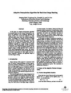
The essential difference between the AIDW algorithm and the standard IDW algorithm is that: in the standard IDW the parameter power α is specified to a constant value (e.g., 2 or 3.0) for all the interpolation points, while in contrast in the AIDW the power α is adaptively determined according to the distribution of the interpolated points and data points. In short, in IDW the power α is user-specified and constant before interpolating; but in AIDW the power α is no longer user-specified or constant but adaptively determined in the interpolating. The main steps of adaptive determining the power α in the AIDW have been listed in subsection 2.2. Among these steps, the most computationally intensive step is to find the k nearest neighbors (kNN) for each interpolated point. Several effective kNN algorithms have been developed by region partitioning using various data structures.20, 33–35 However, these algorithms are computationally complex in practice, and are not suitable to be used in implementing AIDW. This is because that in AIDW the kNN search has to be executed within a single CUDA thread rather than a thread block or grid. In this paper, we present a straightforward but suitable for the GPU parallelized algorithm to find the k nearest data points for each interpolated point. Assuming there are n interpolated points and m data points, for each interpolated point we carry out the following steps: Step 1: Calculate the first k distances between the first k data points and the interpolated points; for example, if the k is set to 10, then there are 10 distances needed to be calculated; see the row (A) in Figure 1. Step 2: Sort the first k distances in ascending order; see the row (B) in Figure 1. Step 3: For each of the rest (m − k) data points, 1) Calculate the distance dist, for example, the distance is 4.8 (dist = 4.8); 2) Compare the dist with the kth distance: if dist < the kth distance, then replace the kth distance with the dist (see row (C)) 3) Iteratively compare and swap the neighboring two distances from the kth distance to the 1st distance until all the k distances are newly sorted in ascending order; see the rows (C) ∼ (G) in Figure 1. Original
6.5
0.7
1.3
2.8
5.2
3.3
8.5
9.1
4.6
7.9
(A)
Sorted
0.7
1.3
2.8
3.3
4.6
5.2
6.5
7.9
8.5
9.1
(B)
Replaced
0.7
1.3
2.8
3.3
4.6
5.2
6.5
7.9
8.5
4.8
(C)
Swapped
0.7
1.3
2.8
3.3
4.6
5.2
6.5
7.9
4.8
8.5
(D)
Swapped
0.7
1.3
2.8
3.3
4.6
5.2
6.5
4.8
7.9
8.5
(E)
Swapped
0.7
1.3
2.8
3.3
4.6
5.2
4.8
6.5
7.9
8.5
(F)
Desired
0.7
1.3
2.8
3.3
4.6
4.8
5.2
6.5
7.9
8.5
(G)
Figure 1. Demonstration of the finding of k nearest neighbors (k = 10) 3.1.3 The Use of Different Data Layouts
Data layout is the form in which data should be organized and accessed in memory when operating on multi-valued data such as sets of 3D points. The selecting of appropriate data layout is a crucial issue in the development of GPU accelerated applications. The efficiency performance of the same GPU application may drastically differ due to the use of different types of data layout. Typically, there are two major choices of the data layout: the Array of Structures (AoS) and the Structure of Arrays (SoA);36 see Figure 2. Organizing data in AoS layout leads to coalescing issues as the data are interleaved. In contrast, the organizing of data according to the SoA layout can generally make full use of the memory bandwidth due to no data interleaving. In addition, global memory accesses based upon the SoA layout are always coalesced. 5/15
In practice, it is not always obvious which data layout will achieve better performance for a specific GPU application. A common solution is to implement a specific application using above two layouts separately and then compare the performance. In this work, we will evaluate the performance impact of the above two basic data layouts and other layouts that are derived from the above two layouts.
struct Pt { float x[N]; float y[N]; float z[N]; }; struct Pt myPts; (a) SoA
struct __align__(16) Pt { float x, y, z; /* plus hidden 32bit padding element */ }; struct Pt myPts[N]; (b) AoaS
Figure 2. Data Layouts SoA and AoaS
3.2 Implementation Details This subsection will present the details on implementing the GPU-accelerated AIDW interpolation algorithm. We have developed two versions: (1) the naive version that does not take advantage of the shared memory, and (2) the tiled version that exploits the use of shared memory. And for both of the above two versions, two implementations are separately developed according to the two data layouts SoA and AoaS. 3.2.1 Naive Version
In this naive version, only registers and global memory are used without profiting from the use of shared memory. The input data and the output data, i.e., the coordinates of the data points and the interpolated points, are stored in the global memory. Assuming that there are m data points used to evaluate the interpolated values for n prediction points, we allocate n threads to perform the parallelization. In other words, each thread within a grid is responsible to predict the desired interpolation value of one interpolated point. A complete CUDA kernel is listed in Figure 3. The coordinates of all data points and prediction points are stored in the arrays REAL dx[dnum], dy[dnum], dz[dnum], ix[inum],iy[inum], and iz[inum]. The word REAL is defined as float and double on single and double precision, respectively. Within each thread, we first find the k nearest data points to calculate the robs (see Equation (3)) according to the straightforward approach introduced in subsection 3.1.2 Method for Finding the Nearest Data Points; see the piece of code from line 11 to line 34 in Figure 3; then we compute the rexp and R (S0 ) according to Equations (2) and (4). After that, we normalize the R (S0 ) measure to µR such that µR is bounded by 0 and 1 by a fuzzy membership function; see Equation (5) and the code from line 38 to line 40 in Figure 3. Finally, we determine the distance-decay parameter α by mapping the µR values to a range of α by a triangular membership function; see Equation (6) and the code from line 42 to line 49. After adaptively determining the power parameterα , we calculate the distances to all the data points again; and then according to the distances and the determined power parameter α , all the m weights are obtained; finally, the desired interpolation value is achieved via the weighting average. This phase of calculating the weighting average is the same as that in the standard IDW method. Note that, in the naive version, it is needed to compute the distances from all data points to each prediction point twice. The first time is carried out to find the k nearest neighbors/data points, see the code from line 11 to line 32; and the second is to calculate the distance-inverse weights; see the code from line 52 to line 57. 6/15
� � � � � � � � � �� �� �� �� �� �� �� �� �� �� �� �� �� �� �� �� �� �� �� �� �� �� �� �� �� �� �� �� �� �� �� �� �� �� �� �� �� �� �� �� �� �� �� �� �� �� �� �� �� �� ��
BBJOREDOBB YRLG�$,':B.HUQHOB1DLYHB6R$�5($/� �G[��5($/� �G\��5($/� �G]��LQW�GQXP������'DWD�SRLQWV ���������������������������5($/� �L[��5($/� �L\��5($/� �L]��LQW�LQXP������,QWHUSODWHG�SRLQWV ���������������������������5($/�DHUDB$ �����������������������������������$UHD�RI�SODQDU�UHJLRQ ^ ����LQW�WLG� �EORFN,G[�[� �EORFN'LP�[���WKUHDG,G[�[� � LI�WLG���LQXP �^ ��������5($/�G>N11@��VXP� ����GLVW� ����W� ����]� ����DOSKD� ��������IRU�LQW�L� ����L���N11��L�� ����'LVWDQFHV�RI�WKH�ILUVW�N11�SRLQWV ������������G>L@� ��L[>WLG@���G[>L@ � ��L[>WLG@���G[>L@ �� ��������������������L\>WLG@���G\>L@ � ��L\>WLG@���G\>L@ �� ��������IRU�LQW�L� ����L���N11������L�� �����6RUW�LQ�DVFHQGLQJ�RUGHU ������������IRU��LQW�M� ����M���N11�������L��M�� � ����������������LI�G>M@�!�G>M����@ �^ ��������������������GLVW� �G>M@���G>M@� �G>M����@���G>M����@� �GLVW� ����������������` ��������IRU�LQW�L� �N11��L���GQXP��L�� �^����$OO�GLVWDQFHV ������������GLVW� ��L[>WLG@���G[>L@ � ��L[>WLG@���G[>L@ �� ��������������������L\>WLG@���G\>L@ � ��L\>WLG@���G\>L@ �� ������������LI�GLVW���G>N11��@ �^�����3RWHQWLDO�QHDUHVW�QHLJKERU ����������������G>N11��@� �GLVW�������5HSODFH�WKH�ODVW�GLVWDQFH ����������������IRU�LQW�M� ����M���N11������M�� �^�����6RUW�DJDLQ�E\�VZDSSLQJ ��������������������LI�G>M@�!�G>M����@ �^ ������������������������GLVW� �G>M@���G>M@� �G>M����@���G>M����@� �GLVW� ��������������������` � � � � ` ������������` ��������` ��������IRU�LQW�L� ����L���N11��L�� �VXP�� �VTUW�G>L@ � ��������5($/�UBREV� �VXP���N11� ��������5($/�UBH[S� ��������� VTUW�GQXP���DHUDB$ ��� ��������5($/�5B6��� �UBREV���UBH[S� ��������5($/�XB5� ��� � � LI�5B6��! �5BPLQ �XB5� ���������� FRV�����������5BPD[ �5B6��5BPLQ � ��������LI�5B6��! �5BPD[ �XB5� ����� � � ���$GDSWLYH�SRZHU�SDUDPHWHU��D��DOSKD ��������LI�XB5! ��� �XB5� ��� ��DOSKD� �D��� ��������LI�XB5!���� �XB5� ��� ��DOSKD� �D� ���� �XB5���� ���D� � �XB5���� � ��������LI�XB5!���� �XB5� ��� ��DOSKD� �D� � �XB5���� ���D� ���� �XB5���� � ��������LI�XB5!���� �XB5� ��� ��DOSKD� �D� ���� �XB5���� ���D� � �XB5���� � ��������LI�XB5!���� �XB5� ��� ��DOSKD� �D� � �XB5���� ���D� ���� �XB5���� � � ����LI�XB5!���� �XB5� ��� ��DOSKD� �D�� � � DOSKD� ���������+DOI�RI�WKH�SRZHU��WR�DYRLG�VTUW�GLVW � � ���:HLJKWHG�DYHUDJH ��������]� ����VXP� ��� ��������IRU�LQW�M� ����M���GQXP��M�� �^ ������������GLVW� ��L[>WLG@���G[>M@ � ��L[>WLG@���G[>M@ �� ��������������������L\>WLG@���G\>M@ � ��L\>WLG@���G\>M@ �� ������������W� ��������SRZ�GLVW��DOSKD ���VXP�� �W���]�� �G]>M@� �W� ��������` ��������L]>WLG@� �]���VXP� � ` `
Figure 3. A CUDA kernel of the naive version of GPU-accelerated AIDW
7/15
3.2.2 Tiled Version
The workflow of this tiled version is the same as that of the naive version. The major difference between the two versions is that: in this version, the shared memory is exploited to improve the computational efficiency. The basic ideas behind this tiled version are as follows. The CUDA kernel presented in Figure 3 is a straightforward implementation of the AIDW algorithm that does not take advantage of shared memory. Each thread needs to read the coordinates of all data points from global memory. Thus, the coordinates of all data points are needed to be read n times, where n is the number of interpolated points. In GPU computing, a quite commonly used optimization strategy is the “tiling,” which partitions the data stored in global memory into subsets called tiles so that each tile fits into the shared memory.14 This optimization strategy “tiling” is adopted to accelerate the AIDW interpolation: the coordinates of data points are first transferred from global memory to shared memory; then each thread within a thread block can access the coordinates stored in shared memory concurrently. In the tiled version, the tile size is directly set as the same as the block size (i.e., the number of threads per block). Each thread within a thread block takes the responsibilities to loading the coordinates of one data point from global memory to shared memory and then computing the distances and inverse weights to those data points stored in current shared memory. After all threads within a block finished computing these partial distances and weights, the next piece of data in global memory is loaded into shared memory and used to calculate current wave of partial distances and weights. It should be noted that: in the tiled version, it is needed to compute the distances from all data points to each prediction point twice. The first time is carried out to find the k nearest neighbors/data points; and the second is to calculate the distance-inverse weights. In this tiled version, both of the above two waves of calculating distances are optimized by employing the strategy “tiling”. By employing the strategy “tiling” and exploiting the shared memory, the global memory access can be significantly reduced since the coordinates of all data points are only read (n/threadsPerBlock) times rather than n times from global memory, where n is the number of predication points and threadsPerBlock denotes the number of threads per block. Furthermore, as stated above the strategy “tiling” is applied twice. After calculating each wave of partial distances and weights, each thread accumulates the results of all partial weights and all weighted values into two registers. Finally, the prediction value of each interpolated point can be obtained according to the sums of all partial weights and weighted values and then written into global memory.
4 Results To evaluate the performance of the GPU-accelerated AIDW method, we have carried out several groups of experimental tests on a personal laptop computer. The computer is featured with an Intel Core i7-4700MQ (2.40GHz) CPU, 4.0 GB RAM memory, and a graphics card GeForce GT 730M. All the experimental tests are run on OS Windows 7 Professional (64-bit), Visual Studio 2010, and CUDA v7.0. Two versions of the GPU-accelerated AIDW, i.e., the naive version and the tiled version, are implemented with the use of both the data layouts SoA and AoaS. These GPU implementations are evaluated on both the single precision and double precision. However, the CPU version of the AIDW implementation is only tested on double precision; and all results of this CPU version are employed as the baseline results for comparing computational efficiency. All the data points and prediction points are randomly created within a square. The numbers of predication points and the data points are equivalent. We use the following five groups of data size, i.e., 10K, 50K, 100K, 500K, and 1000K, where one K represents the number of 1024 (1 K = 1024). For the GPU implementations, the recorded execution time includes the cost spent on transferring the input data point from the host to the device and transferring the output data from the device back to the host; but it does not include time consumed in creating the test data. Similarly, for the CPU implementation, the time spent for generating test data is also not considered. 8/15
4.1 Single Precision The execution time of the CPU and GPU implementations of the AIDW on single precision is listed in Table 1. And the speedups of the GPU implementations over the baseline CPU implementation are illustrated in Figure 4. According to these testing results, we have observed that: (1) The speedup is about 100 ∼ 400; and the highest speedup is up to 400, which is achieved by the tiled version with the use of the data layout SoA; (2) The tiled version is about 1.45 times faster than the naive version; (3) The data layout SoA is slightly faster than the layout AoaS. In the experimental test when the number of the data points and interpolation points is about 1 million (1000K = 1024000), the execution time of the CPU version is more than 18 hours, while in contrast the tiled version only needs less than 3 minutes. Thus, to be used in practical applications, the tiled version of the GPU-accelerated AIDW method on single precision is strongly recommended. Version
Data Layout
CPU
SoA AoaS SoA AoaS
GPU Naive GPU Tiled
10K 6791 65.3 66.3 61.3 61.6
Data Size (1K = 1024) 50K 100K 500K 168234 673806 16852984 863 2884 63599 875 2933 64593 714 2242 43843 722 2276 44891
1000K 67471402 250574 254488 168189 172605
Table 1. Execution time (/ms) of CPU and GPU implementations of the AIDW method on single precision
500 384.39
400
401.16
Speedup
300.54 300 Naive SoA
235.62
Naive AoaS
200
Tiled SoA
110.78 100
Tiled AoaS
0 10K
50K
100K
500K
1000K
Data Size (1K = 1024)
Figure 4. Speedups of the GPU-accelerated AIDW method on single
4.2 Double Precision We also evaluate the computational efficiency of the naive version and the tiled version on double precision. It is widely known that the arithmetic operated on GPU architecture on double precision is inherently much slower than that on single precision. In our experimental tests, we also clearly observed this behavior: on double precision, the 9/15
speedup of the GPU version over the CPU version is only about 8 (see Figure 5), which is much lower than that achieved on single precision. We have also observed that: (1) there are no performance gains obtained from the tiled version against the naive version; and (2) the use of data layouts, i.e., SoA and AoaS, does not lead to significant differences in computational efficiency. As observed in our experimental tests, on double precision the speedup generated in most cases is approximately 8, which means the GPU implementations of the AIDW method are far from practical usage. Thus, we strongly recommend users to prefer the GPU implementations on single precision for practical applications. In the subsequent section, we will only discuss the experimental results obtained on single precision. 10
Speedup
9 8 Naive SoA Naive AoaS
7
Tiled SoA 6
Tiled AoaS
5 10K
50K
100K
500K
1000K
Data Size (1K = 1024)
Figure 5. Speedups of the GPU-accelerated AIDW method on double precision
5 Discussion 5.1 Impact of Data Layout on the Computational Efficiency In this work, we have implemented the naive version and the tiled version with the use of two data layouts SoA and AoaS. In our experimental tests, we have found that the SoA data layout can achieve better efficiency than the AoaS. However, there is no significant difference in the efficiency when using the above two data layouts. More specifically, the SoA layout is only about 1.015 times faster than the AoaS for both the naive version and the tiled version; see Figure 6. As stated in Section 3, organizing data in AoaS layout leads to coalescing issues as the data are interleaved. In contrast, the organizing of data according to the SoA layout can generally make full use of the memory bandwidth due to no data interleaving. In addition, global memory accesses based upon the SoA layout are always coalesced. This is perhaps the reason why the data layout SoA can achieve better performance than the AoaS in our experimental tests. However, it also should be noted that: it is not always obvious which data layout will achieve better performance for a specific application. In this work, we have observed that the layout SoA is preferred to be used, while in contrast the layout AoaS is suggested to be employed in our previous work.31 5.2 Performance Comparison of the Naive Version and Tiled Version In our experimental tests, we also observed that the tiled version is about 1.3 times faster than the naive version on average no matter which data layout is adopted; see Figure 7. This performance gain is due to the use of shared 10/15
Speedup of SoA Layout against AoaS Layout 1.030 1.025 1.026 Speedup
1.020
1.017 1.015
1.024 1.016
1.016
1.014
1.015 Naive
1.015 1.010
Tiled
1.011 1.005 1.005 1.000 10K
50K
100K
500K
1000K
Data Size (1K = 1024)
Figure 6. Performance comparison of the layouts SoA and AoaS memory according to the optimization strategy “tiling”. On GPU architecture, the shared memory is inherently much faster than the global memory; thus any opportunity to replace global memory access by shared memory access should therefore be exploited. In the tiled version, the coordinates of data points originally stored in global memory are divided into small pieces/tiles that fit the size of shared memory, and then loaded from slow global memory to fast shared memory. These coordinates stored in shared memory can be accessed quite fast by all threads within a thread block when calculating the distances. By blocking the computation this way, we take advantage of fast shared memory and significantly reduce the global memory accesses: the coordinates of data points are only read (n/threadsPerBlock) times from global memory, where n is the number of prediction points. This is the reason why the tiled version is faster than the naive version. Therefore, from the perspective of practical usage, we recommend the users to adopt the tiled version of the GPU implementations. 5.3 Comparison of GPU-accelerated AIDW, IDW, and Kriging Methods In the literature,32 Lu and Wong has analyzed the accuracy of sequential AIDW with the standard IDW and the Kriging method. They focused on illustrating the effectiveness of the proposed AIDW method. However, in this work, we intend to present a parallel AIDW with the use of the GPU; and here we focus on comparing the efficiency of the GPU-accelerated AIDW with the corresponding parallel version of IDW and Kriging method. 5.3.1 AIDW vs. IDW
First, we compare the GPU-accelerated AIDW with the standard IDW. The AIDW is obviously more computationally expensive than the IDW. The root cause of this behavior is also quite clear: in AIDW it is needed to dynamically determine the adaptive power parameter according to the spatial points’ distribution pattern during interpolating, while in IDW the power parameter is statically set before interpolating. Due to the above reason, in the GPU-accelerated AIDW, each thread needs to perform much more computation than that in the IDW. One of the obvious extra computational steps in the GPU-accelerated AIDW is to find some nearest neighbors, which needs to loop over all the data points. This means in the AIDW each thread needs to calculate the distances from all the data points to one interpolated point twice: the first time is to find the nearest neighbors and the second is to obtain the distance-inverse weights. In contrast, in the IDW each thread is only invoked to calculate the distances once. 11/15
Speedup of Tiled Version against Naive Version 1.6 1.490 1.451
1.5 Speedup
1.4 1.286 1.3 1.209
SoA
1.2 AoaS 1.1
1.065
1.0 10K
50K
100K
500K
1000K
Data Size (1K = 1024)
Figure 7. Performance comparison of the naive version and tiled version
5.3.2 AIDW vs. Kriging
Second, we compare the GPU-accelerated AIDW with the Kriging method. Although the AIDW is by nature computationally expensive than the IDW, it is still computationally inexpensive than the Kriging method. In Kriging, the desired prediction value of each interpolated point is also the weighted average of data points. The essential difference between the Kriging interpolation and the IDW and AIDW is that: in Kriging the weights are calculated by solving a linear system of equations, while in both IDW and AIDW the weights are computed according to a function in which the parameter is the distance between points. As stated above, in Kriging the weights are achieved by solving a linear system of equations, AV = B, where A is the matrix of the semivariance between points, V is the matrix of weights and B stands for the variogram. Thus, in fact, the Kriging method can be divided into three main steps: (1) the assembly of A, (2) the solving of AV = B, and (3) the weighting average. The third step is the same as those in both IDW and AIDW. The most computationally intensive steps are the assembly of A and the solving of AV = B. Each entry of the matrix A is calculated according to the so-called semivariance function. The input parameter of the semivariance function is the distance between data points. Thus, in GPU-accelerated Kriging method, when each thread is invoked to compute each row of the matrix A, it is needed to loop over all data points for each thread to first calculate the distances and then the semivariances. Obviously, the assembly of the matrix A can be performed in parallel by allocating m threads, where m is the number of data points. Another key issue in assembling the matrix A is the storage. In AIDW, the coordinates of all the data points and interpolated points are needed to be stored in global memory. There is no other demand for storing the large size of intermediate data during interpolating. However, in Kriging the matrix A needs to be additionally stored during interpolating. The matrix A is a square matrix with the size of at least (m+1)× (m+1), where m is the number of data points. Moreover, in general the A is dense rather than sparse, which means the matrix A cannot be stored in any compressed formats such as COO (COOrdinate) or CSR (Compressed Sparse Row). Thus, the global memory accesses in Kriging are much more than those in AIDW due to the storing of the matrix A. This will definitely increase the computational cost. As mentioned above, the vector of weights V can be obtained by solving the equations AV = B. But in fact the vector can be calculated according to V = A−1 B. This means the matrix A is only needed to be inverted once, 12/15
and then repeatedly used. However, to obtain the vector of weights V, first the inverse of the matrix A and then the matrix multiplication is needed to be carried out. The matrix inverse is only needed to be performed once; but the matrix multiplication has to be carried out for each interpolated point. In GPU-accelerated Kriging method, when a thread is invoked to predict the value of one interpolated point, then each thread needs to perform the matrix multiplication V = A−1 B. The classical matrix multiplication algorithm is computationally expensive in CPU as a consequence of having an O(n3 ) complexity. And, the complexity of the matrix multiplication algorithm in a GPU is still O(n2 ).18 This means in GPU-accelerated Kriging method, each thread needs to perform the computationally expensive step of matrix multiplication. In contrast, in GPUaccelerated AIDW, the most computationally expensive step is the finding of nearest neighbors, which only has the complexity of O(n).
6 Conclusions On a single GPU, we have developed two versions of the GPU-accelerated AIDW interpolation algorithm, the naive version that does not profit from shared memory and the tiled version that takes advantage of shared memory. We have also implemented the naive version and the tiled version with the use of two data layouts, AoS and AoaS, on both single precision and double precision. We have demonstrated that the naive version and the tiled version can approximately achieve the speedups of about 270 and 400 on single precision, respectively. In addition, on single precision the implementations using the layout SoA are always slightly faster than those using the layout AoaS. However, on double precision, the overall speedup is only about 8; and we have also observed that: (1) there are no performance gains obtained from the tiled version against the naive version; and (2) the use of data layouts, i.e., SoA and AoaS, does not lead to significant differences in computational efficiency. Therefore, the tiled version that is developed using the layout SoA on single precision is strongly recommended to be used in practical applications.
Acknowledgements This research was supported by the Natural Science Foundation of China (Grant No. 40602037 and 40872183), China Postdoctoral Science Foundation (2015M571081), and the Fundamental Research Funds for the Central Universities (2652015065).
References 1. Shepard, D. A two-dimensional interpolation function for irregularly-spaced data (1968). 2. Krige, D. G. A statistical approach to some basic mine valuation problems on the witwatersrand. Journal of the Chemical, Metallurgical and Mining Society of South Africa 52, 119–139 (1951). 3. Mallet, J. L. Discrete smooth interpolation. Acm Transactions on Graphics 8, 121–144 (1989). Times Cited: 86 0 101. 4. Mallet, J. L. Discrete smooth interpolation in geometric modeling. Computer-Aided Design 24, 178–191 (1992). Times Cited: 107 0 123. 5. Mei, G. Summary on several key techniques in 3d geological modeling. Scientific World Journal (2014). Times Cited: 1 Mei, Gang/0000-0003-0026-5423 0 1. 6. Falivene, O., Cabrera, L., Tolosana-Delgado, R. & Saez, A. Interpolation algorithm ranking using crossvalidation and the role of smoothing effect. a coal zone example. Computers & Geosciences 36, 512–519 (2010). Falivene, Oriol Cabrera, Lluis Tolosana-Delgado, Raimon Saez, Alberto Saez, Alberto/K-4269-2012 Saez, Alberto/0000-0003-4215-5038. 7. Armstrong, M. P. & Marciano, R. J. Inverse distance weighted spatial interpolation using a parallel supercomputer. Photogrammetric Engineering and Remote Sensing 60, 1097–1103 (1994). 8. Armstrong, M. P. & Marciano, R. J. Massively parallel strategies for local spatial interpolation. Computers & Geosciences 23, 859–867 (1997). Armstrong, MP Marciano, RJ. 13/15
9. Guan, X. F. & Wu, H. Y. Leveraging the power of multi-core platforms for large-scale geospatial data processing: Exemplified by generating dem from massive lidar point clouds. Computers & Geosciences 36, 1276–1282 (2010). Guan, Xuefeng Wu, Huayi. 10. Guan, Q. F., Kyriakidis, P. C. & Goodchild, M. F. A parallel computing approach to fast geostatistical areal interpolation. International Journal of Geographical Information Science 25, 1241–1267 (2011). Guan, Qingfeng Kyriakidis, Phaedon C. Goodchild, Michael F. SI. 11. Wang, S.-Q., Gao, X. & Yao, Z.-X. Accelerating pocs interpolation of 3d irregular seismic data with graphics processing units. Computers & Geosciences 36, 1292–1300 (2010). 12. Kerry, K. E. & Hawick, K. A. Kriging interpolation on high-performance computers, vol. 1401 of Lecture Notes in Computer Science, 429–438 (1998). Kerry, KE Hawick, KA International Conference and Exhibition on High-Performance Computing and Networking APR 21-23, 1998 AMSTERDAM, NETHERLANDS Hawick, Ken/E-1609-2013 Hawick, Ken/0000-0002-2447-3940.
13. Henneb¨ohl, K., Appel, M. & Pebesma, E. Spatial interpolation in massively parallel computing environments (2011). URL http://itcnt05.itc.nl/agile_old/Conference/2011-utrecht/contents/pdf/shortpapers/s 14. Pesquer, L., Cortes, A. & Pons, X. Parallel ordinary kriging interpolation incorporating automatic variogram fitting. Computers & Geosciences 37, 464–473 (2011). Pesquer, Lluis Cortes, Ana Pons, Xavier Cortes, Ana/J-6299-2014; Pons, Xavier/N-1202-2014 Cortes, Ana/0000-0003-1697-1293; Pons, Xavier/0000-00026924-1641. 15. Strzelczyk, J. & Porzycka, S. Parallel Kriging Algorithm for Unevenly Spaced Data, vol. 7133 of Lecture Notes in Computer Science, 204–212 (2012). Strzelczyk, Jacek Porzycka, Stanislawa 10th Nordic International Conference on Applied Parallel Computing - State of the Art in Scientific and Parallel Computing (PARA) JUN 06-09, 2010 Reykjavik, ICELAND CCP, Microsoft Islandi, Opin kerfi (Hewlett Packard Distributor Iceland). 16. Cheng, T. P. Accelerating universal kriging interpolation algorithm using cuda-enabled gpu. Computers & Geosciences 54, 178–183 (2013). Cheng, Tangpei. 17. Shi, X. & Ye, F. Kriging interpolation over heterogeneous computer architectures and systems. Giscience & Remote Sensing 50, 196–211 (2013). Shi, Xuan Ye, Fei. 18. de Rave, E. G., Jimenez-Hornero, F. J., Ariza-Villaverde, A. B. & Gomez-Lopez, J. M. Using general-purpose computing on graphics processing units (gpgpu) to accelerate the ordinary kriging algorithm. Computers & Geosciences 64, 1–6 (2014). Gutierrez de Rave, E. Jimenez-Hornero, F. J. Ariza-Villaverde, A. B. GomezLopez, J. M. Jimenez-Hornero, Francisco/K-8771-2014 Jimenez-Hornero, Francisco/0000-0003-4498-8797. 19. Hu, H. D. & Shu, H. An improved coarse-grained parallel algorithm for computational acceleration of ordinary kriging interpolation. Computers & Geosciences 78, 44–52 (2015). Hu, Hongda Shu, Hong. 20. Wei, H. T. et al. A k-d tree-based algorithm to parallelize kriging interpolation of big spatial data. Giscience & Remote Sensing 52, 40–57 (2015). Wei, Haitao Du, Yunyan Liang, Fuyuan Zhou, Chenghu Liu, Zhang Yi, Jiawei Xu, Kaihui Wu, Di. 21. Huang, F. et al. Explorations of the implementation of a parallel idw interpolation algorithm in a linux clusterbased parallel gis. Computers & Geosciences 37, 426–434 (2011). 22. Li, L. X., Losser, T., Yorke, C. & Piltner, R. Fast inverse distance weighting-based spatiotemporal interpolation: A web-based application of interpolating daily fine particulate matter pm2.5 in the contiguous u.s. using parallel programming and k-d tree. International Journal of Environmental Research and Public Health 11, 9101–9141 (2014). Li, Lixin Losser, Travis Yorke, Charles Piltner, Reinhard.
23. NVIDIA. Cuda c programming guide v7.0 (2015). URL http://docs.nvidia.com/cuda/cuda-c-programmin 24. Munshi, A. The opencl specification, version: 2.0 (2013). 14/15
25. Huraj, L., Sil´adi, V. & Sil´acˇ i, J. Comparison of design and performance of snow cover computing on gpus and multi-core processors. WSEAS Transactions on Information Science and Applications 7, 1284–1294 (2010). 26. Huraj, L., Sil´adi, V. & Sil´aci, J. Design and performance evaluation of snow cover computing on gpus (2010). 27. Hanzer, F. Spatial interpolation of scattered geoscientific data (2012). URL http://www.uni-graz.at/˜haasegu/Lectures/GPU_CUDA/WS11/hanzer_report.pdf. 28. Xia, Y., Kuang, L. & Li, X. Accelerating geospatial analysis on gpus using cuda. Journal of Zhejiang University SCIENCE C 12, 990–999 (2011). 29. Xia, Y., Shi, X., Kuang, L. & Xuan, J. Parallel geospatial analysis on windows hpc platform (2010). 30. Mei, G. Evaluating the power of gpu acceleration for idw interpolation algorithm. Scientific World Journal (2014). Mei, Gang Mei, Gang/0000-0003-0026-5423. 31. Mei, G. Impact of data layouts on the efficiency of gpu-accelerated idw interpolation. SpringerPlus (2015). 32. Lu, G. Y. & Wong, D. W. An adaptive inverse-distance weighting spatial interpolation technique. Computers & Geosciences 34, 1044–1055 (2008). Lu, George Y. Wong, David W. 33. Leite, P. et al. Nearest neighbor searches on the gpu a massively parallel approach for dynamic point clouds. International Journal of Parallel Programming 40, 313–330 (2012). Leite, Pedro Teixeira, Joao Marcelo Farias, Thiago Reis, Bernardo Teichrieb, Veronica Kelner, Judith SI. 34. Huang, H., Cui, C., Cheng, L., Liu, Q. & Wang, J. Grid interpolation algorithm based on nearest neighbor fast search. Earth Science Informatics 5, 181–187 (2012). 35. Dashti, A., Komarov, I. & D’Souza, R. M. Efficient computation of k-nearest neighbour graphs for large high-dimensional data sets on gpu clusters. Plos One 8 (2013). Dashti, Ali Komarov, Ivan D’Souza, Roshan M. 36. Farber, R. Chapter 6 - Efficiently Using GPU Memory, 133–156 (Morgan Kaufmann, Boston, 2011).
15/15