ACCOUNTABILITY AND ERROR IN ENSEMBLE FORECASTING ..... The last entry in the list above (denoted by a \ ") re ects the separate requirement, for a ...
ACCOUNTABILITY AND ERROR IN ENSEMBLE FORECASTING Leonard A Smith
Mathematical Institute, University of Oxford Oxford, England ABSTRACT Forecast evaluation based on single predictions, each determined from an imperfectly observed initial state, is incomplete; observational uncertainty implies that an ensemble of initial states of the system is consistent with a given observation. In a nonlinear system, this initial distribution will develop a non-Gaussian structure, even if the forecast model is perfect. A perfect prediction (that is, forecasting the future state of the system) from an uncertain initial observation, is not possible even with a perfect model. Yet this irreducible uncertainty is accountable, in that it is distinct from model error. Ensemble prediction of nonlinear systems reveals shortcomings in the traditional evaluation of forecast-veri cation pairs with least-squared error cost functions; an alternative evaluation of imperfect models through their ability to shadow uncertain observations is discussed. Di�culties surrounding the construction of an ensemble of initial conditions are considered, the implications of imperfect ensembles are noted, and the use of breeding vectors and singular vectors is contrasted in low-dimensional systems. 1.
INTRODUCTION
While predictions founded upon less than perfect observations will always be in error, we can strive to account for the origin of forecast errors. In particular, we can attempt to determine the extent to which shortcomings are due (1) to misinterpreting the accuracy of the observations, (2) to model error, or (3) to the limited computational resources available. To be self-consistent, nonlinear prediction schemes must account for observational uncertainty both when tuning the forecast model and when interpreting each observation from which a forecast is initiated. This may be done, for example, by considering an ensemble of initial conditions, each of which is consistent with a given observation (see, for example, Epstein, 1969, Leith, 1974, Ho�man and Kalnay, 1983, Murphy, 1988, Palmer, 1992, Tracton and Kalnay, 1993, Ehrendorfer, 1994 and references thereof). Item (3) in this list di�ers from the others in that it is primarily a technical (or at least, a technological) constraint. To the extent that the shortcoming of a forecasting system is due to (3), we shall say it is accountable; the frequency of occurrence of unanticipated events can be estimated, and reduced through the commitment of additional resources. To the extent that this is not the case, the forecast is in error, and improvement of the model and/or the interpretation of the observations is needed. Perfect models, given perfect ensembles (de ned below), are always accountable, although in regions of great sensitivity to initial condition, their forecasts may be of limited utility. The importance of the role played by uncertainty in the initial condition has been recognised in numerical weather forecasting for some time (e.g. Thompson, 1957). Below, we will restrict attention to low-order systems where the application of nonlinear dynamical systems theory can be put to the test using ensembles which are orders of magnitude larger than those practical in numerical weather forecasting models. Generally, we will plot a single observable, s, and consider an ensemble of initial conditions, each consistent with the uncertainty of an observation in state-space. Note that as long as digital computers are involved, the e�ects of observational uncertainty are unavoidable even in principle; at the very least, there will be truncation errors due to an analog-to-digital (A/D) conversion. As the initial uncertainty in the true value of s evolves with time, we can treat the evolution of the ensemble as a forecast by interpreting the distribution of the ensemble points as the probability density function (PDF) of s after time t, which we denote as (s). The evolution of (s) with time for several chaotic systems is shown in the rst three gures. When both the model dynamics and the ensemble are perfect, we have an optimal forecast for a given deterministic t
t
system; the statistical aspect is unavoidable. Our incomplete knowledge of the initial conditions forces the probabilistic interpretation even when we know the exact deterministic dynamics. For chaotic systems, (s) may, or may not, \quickly" spread over the full range of s; given a perfect model, it will eventually evolve toward an invariant PDF, 1 (s). In the absence of any knowledge of the current state of the system, our best prediction is summarized by 1 (s) (i.e. the climatological distribution or equivalently, the projection of the invariant measure (\the attractor") onto the variable we are observing). t
Initially, one may observe an exponential growth of uncertainty; while this must stop when the uncertainty is comparable with the diameter of the attractor, saturation may occur at any nite length scale (in particular, at arbitrarily small length scales) and persist for arbitrarily long times. The \average exponential growth" of chaotic systems is a globally averaged rate based on in nitesimal uncertainties; it places no a priori limits whatsoever upon operational predictability, or upon the local growth rates which can, and often do, correspond to decreasing uncertainty (for nite times) in chaotic systems. 2.
OPTIMAL FORECAST SCENARIO
To isolate the various limitations on predictability, rst consider the optimal forecast scenario: a perfect model of the dynamics, an exact understanding of the origin of observational uncertainty, and a perfect ensemble of initial conditions. The perfect model scenario is a common one: we will use, for example, the Lorenz equations (Lorenz, 1963) to predict data generated from the Lorenz equations. For simplicity, we take the observational uncertainty to be due only to nite accuracy - that is, we observe the true value of each variable, but only to a xed number of digits. The uncertainty is then due to truncation error. This e�ectively divides the state-space of the system into a mesh of hyper-cubes; our observation tells us which cube the system is in, but says nothing as to where within the cube it is. As we shall see, for systems evolving on attractors this is a serious limitation. We lift this constraint by considering a perfect ensemble; that is, an ensemble of initial conditions which are not only within the correct hyper-cube, but also on the attractor. To construct such an ensemble for a speci c initial condition, we follow the advice given in Lorenz (1963): we \simply" integrate the system of interest and collect exact analogs, exact that is, to within our measurement accuracy (points within the same hyper-cube, and also on the attractor). Armed with this ensemble of analogs (and observations of their future trajectories), we can make an optimal forecast for this initial observation. An example for the Lorenz 1963 system is given in Figure 1. Time increases from bottom to top, in the lower left we see the distribution of values of x at the initial time. All of the initial conditions which are consistent with the current observation lie within the same cube of state-space, hence the initial distribution in x is very sharp. Initially (0 < t < 0:2) the distribution spreads out as might be expected from linear prediction theory. The forecast ensemble then re-sharpens1 showing true \return of skill2 " until t � 0:5; the distribution then oscillates until t � 1:5, when it bifurcates and a substantial fraction of the initial conditions explore each lobe of the attractor. The symmetry of the system results in a false \return of skill" (i.e. at t � 2:3; t � 3:0; and so on) as noted by Palmer (1993). Na�vely, it might appear surprising that any structure should remain in the distribution at t = 12, given that the leading Lyapunov exponent �1 � 1:3 bits per unit time, and the initial conditions were known to only 8 bits. In order to avoid the complications arising from the symmetry and near- atness (the almost 2dimensional structure) of the Lorenz attractor, we shall also consider another three dimensional system of ordinary di�erential equations (Moore and Spiegel, 1966) . The equations, given in the This re ects a nite region of state-space within which all in nitesimal perturbations shrink with time, as established analytically by Ziehmann (1994) for the Lorenz (1963) system, and foreseen for nonlinear systems in general by Tong and Moeanaddin (1988). Also see Ziehmann et al. (1995), Smith (1994a,b) and Smith et al. (1996). 2 See, for example, Anderson and van den Dool (1994). 1
appendix, describe the motion of a parcel of ionized gas in the atmosphere of a star; for the parameters chosen, the system is chaotic with �1 � 0:22 bits per unit time. Figures 2 and 3 show the evolution of several perfect ensembles under a perfect model. In Figure 2, each initial PDF is followed for one unit of time, after which the true state of the system is observed and the PDF collapses onto the new observation3 . A new perfect ensemble is then formed for the t = 1 observation, and the process is repeated. Figure 3 is similar, however the PDF is evolved for 5 units of time between observations. For clarity, the time of each new observation is marked by a vertical gap. These gures show that there are extreme variations in predictability even in these simple lowdimensional models. In Figure 2, the ensembles starting at t = 0; 2 and 8 are broadly dispersed within �t = 1, those at t = 1; 3; 5 and 6 remain fairly tight. The ensemble initiated at t = 7 quickly bifurcates into two packets which remain distinct and fairly well-de ned. The initial ensemble at t = 11 in Figure 3 reveals intermittent return of skill, while the one initiated at t = 16 develops macroscopic structure (i.e. 17:5 < t < 18:5) while remaining fairly coherent until t = 21: On the additional assumption that the initial conditions are chosen uniformly from those in the cube which are on the attractor, the forecasts discussed above are optimal (perfect) in the sense that the future ensemble distribution approximates the true probability distribution function (PDF) of the system, given this initial observation. Unexpected events (deviations from the forecast PDF), are accountable in that their frequency shall decrease in the expected manner as the (perfect) ensemble size increases. Of course, if we knew the exact initial condition, then the PDF would remain a � function for all time; but as the initial observation corresponds to an in nite number of potential initial conditions, we must make probabilistic predictions for this deterministic system. The probabilistic aspect comes only from the uncertainty in observation (there is no inexact computation with analog forecasts). Optimal forecast scenarios are restricted either to systems which we construct, or to those for which observations over many Poincar�e return times are available. For most physical systems this is not possible, and it is interesting to see how a less-than-perfect model fails. The thermally driven, rotating
uid annulus of Read et al. (1992) provides an example of particular interest and relevance. A truly in nite dimensional system, it is believed to exhibit low dimensional, chaotic dynamics; time series of temperature measurements from a co-rotating probe are often analysed (see also R. Smith (1992) and L. Smith (1992)). Figures of ensemble forecasts for a radial basis function model of the thermally driven rotating-annulus are given in Smith (1995). These forecasts are not accountable, indicating variations in model error with initial condition in addition to variations in system sensitivity. In addition to ensemble forecasts which spread out quickly (reminiscent of the forecast from t = 0 to t = 1 at the bottom left panel of Figure 2), there are a signi cant number of forecasts for which the PDF remains coherent (as in the forecast from t = 5 to t = 6 at the bottom right panel of Figure 2), but which give zero probability to the next observed temperature of the annulus (unlike those of Figure 2). The key word here is, of course, \signi cant" which implies large given the number of elements in the ensemble. For the annulus model, the ensemble is not perfect (the initial conditions do not lie on the attractor), and thus it is not clear how to make this relation exact. Indeed, as illustrated in Smith (1995), there exist initial conditions consistent with the observations which lie in a di�erent basin of attraction! Using the annulus as a test case has signi cant advantages over both numerical models and meteorological observations; as a physical system, the same qualitative di�culties arise as in meteorological observations and cannot be circumvented as they often are in numerical studies, either on purpose or by accident; it is an in nite dimensional ( uid) system, imperfectly observed. Yet the physical time scales over which accurate observations can be made is much greater than the (equivalent) time scale for the atmosphere. Extensive ensemble forecasting experiments for this system are now underway This collapse is, of course, only in our uncertainty; the obvious analogy with quantum mechanics is useful but super cial, since in our case the observation does not e�ect the state of the system, it merely (attempts to) re ne our knowledge of it. 3
6.00
12.00
5.50
11.50
5.00
11.00
4.50
10.50
4.00
10.00
3.50
9.50
3.00
9.00
2.50
8.50
2.00
8.00
1.50
7.50
1.00
7.00
0.50
1.00 0.50 0.00
6.50
and shall be reported elsewhere. In the next section, we consider attempts to quantify predictability through the growth rates of in nitesimals, before returning to consider practical methods of forming ensembles in Section 4. 3.
LIMITATIONS OF INFINITESIMALS
It is commonly assumed that chaotic systems are practically unpredictable except in the very near future; in fact, they may be very predictable, except in the exceedingly remote future. The misperception usually arises from a misinterpretation of the constraints implied by a positive Lyapunov exponent. Lyapunov exponents can be understood in terms of the tangent propagator discussed in Section 4. The largest Lyapunov exponent, �1, quanti es the growth rate of almost any in nitesimal uncertainty averaged over the attractor; while it is commonly said that an uncertainty �(t) will grow as �(t) � �(0) exp(�1t), this need be true only as both � ! 0 and t ! 1. In very simple systems we may nd uniform exponential growth, but in general, non-uniformity is the rule on strange attractors, as noted by Benzi et al. (1989). The Lyapunov exponents of a system describe the \e�ective" growth rate of an in nitesimal perturbation, their application to de ning a \limit of predictability" is hampered by two facts: rst, no matter how large an in nitesimal gets, as long as it remains in nitesimal it places no limits on predictability, and as soon as it becomes nite, the Lyapunov exponents cease to describe its evolution. Second, Lyapunov exponents, whether global or nite-time4 , are average rates, and estimating an average time by the inverse of an average rate is somewhat hazardous! Knowing the average velocity of a journey from Oxford to central London via Reading may tell us little about the time required to reach Reading. 3.1
Lyapunov exponents
In practice, it is easy to demonstrate that Lyapunov exponents do not restrict predictability; the Baker's Apprentice Maps presented in Smith (1994a), all have �1 > 1 bit per unit time, while the majority of initial conditions may be predicted with much greater accuracy than the standard Baker's Map for which �1 = 1. It is the inhomogeneity of the Apprentice Maps which gives rise to the enhanced predictability. Similarly, the intuition that an attractor with no positive Lyapunov exponents implies predictability is unfounded; attractors for which in nitesimal uncertainties shrink, may have complicated macroscopic structure within which almost all nite uncertainties grow, sometimes exponentially, for the majority of initial conditions in state-space. As a global averaged rate, �1 need say nothing about the evolution of any nite uncertainty or any xed time. 3.2
Uncertainty Doubling Times
An alternative approach to quantifying predictability is to estimate uncertainty doubling times, �2 (x), or more generally � (x), where � is the time required for an in nitesimal uncertainty to increase by a factor of q . We shall assume that the initial orientation of each in nitesimal uncertainty has been determined by the ow, that is, it is directed in the local orientation of the rst global Lyapunov vector, de ned in Section 4.1 below. The distribution of �2 for the Lorenz attractor is shown in Smith (1994a) and Ziehmann (1994), revealing a banded structure reminiscent of the distribution of the Baker's Apprentice Maps. q
q
There are a variety of con icting de nitions for nite-time or so-called \local" Lyapunov exponents. Our meaning is made clear in Section 4. Alternative points of view may be found in Eckmann et al. (1986), Abarbanel et al. (1991), McCa�rey et al. (1992), Toth and Kalnay, (1995) and the references therein. Note that, as stressed by Wolf et al. (1985) and Oseledec (1968), Lyapunov exponents cannot be de ned in terms of local properties of a dynamical system. 4
5.00
10.00
4.50
9.50
4.00
9.00
3.50
8.50
3.00
8.00
2.50
7.50
2.00
7.00
1.50
6.50
1.00
6.00
0.50
5.50 1.00 0.50 0.00
16.00
21.00
15.50
20.50
15.00
20.00
14.50
19.50
14.00
19.00
13.50
18.50
13.00
18.00
12.50
17.50
12.00
17.00
11.50
16.50 1.00 0.50 0.00
b b b bb bb b b b b b b bb bb bbb b bb b b b bb bb bb bbbbbbb bb b b b bbbbb bbb b b bb b b b bb bb b b b b b bbbb b bbbbbb b b b bbb bbb b bb b b bbb bb bbb bb bb bb b bbbbbb bbbbbbbbbbbbbbbbb b b b b b 40 b b b bb b b b b bbb b b b b b b b bb b bbbb bbbb b b b b b b b b b b b b bbbbb b b bbbbbbbbbbbbbbbbb bb b b b bb bbbbbbbbbbbb bb bbbbbbbbbbbbbbbbb b bb bbbb bbbbbbbb bbbbbbbbbbbb b b b b bbbbbbbb b b b b b b b bbbbbbbbbbb bbbbbbbbbbbbbbbbb b bb bbbb bbbbbbb b bb bbbbbbb bbb bbbbb b bb bbbbb bb bb bbb bbbbb bb bbbbbbbbbbbbb bbbb b b bbbbbbbbbbbbbbbbbbbbbb b b b b b b bbbb b bb + bbbbbbbbbbbbbbbbbbbbbbbbbbbbb b bbbbb bbbbbb b bbb+bbbbbbb b bb bb bbbbbbbbbbbbbb bbbbbbbbbbbbbb bbb bbbb bb bb b b b bbbbbbbbbbbbbb b b b b b bb b b 20 bbbbbbbbbbbbb b b+bbbbbb b b +b bb bbb+b bb bbbb+bbb+b bbbbbb bbb +bb + + + b +bbbb b bb +bbbb++bbbb++bb +bbbbbbbbbb +b b b +b b+bb b +bb++ ++++ + b b b bbbbb b b b + + bb + b bb++bbb bb bb b b ++bbbb bb+b+bbbb b+ ++++b++b+++ + b b +++bbbb++bbb+++bbbbb+bbbb+bbb + + ++bb++++bb++++ ++bbb +bbbb+bbb b ++++++b+++b++b +bbbbbb+b+++bb b b +b+ b+++b+b++ +bbbbbb ++b+++b++b++bbb ++b++bbbbb bb +++++b++ ++bbbbbb++b++++bb+++++++bb++++bb+++b+b++b+++ b + + + + + 0 0 10 20 30 q-pling time
2
q -pling time
60
b
Figure 4. The variation in the uncertainty doubling time as shown by plotting �2 against �4 as `+'; also shown is �32 against �1024 (as `x'). If stretching along the attractor was e�ectively uniform at these time scales, the points should fall along the line y = 2x; which is shown for comparison. Inasmuch as the � directly re ect the time it takes an in nitesimal uncertainty to grow, they are more useful than Lyapunov exponents which de ne average rates over xed periods of time. But the � can be misleading as well. A common motivation for computing the doubling time is to obtain a benchmark for other q ?pling times: if the doubling time is 3 days, one might expect an eight fold increase in 9 days. Such a generalization implicitly assumes a time scale exists on which � 2 (x) � 2� (x). Figure 4 shows that, for the Moore-Spiegel system, this is not the case. This gure plots �2 against �4 , and also �32 against �1024, for a number of initial conditions. The observation that these points do not lie on the line above implies that we cannot generalize from � unless q > 32 (at least), which in turn, requires that our uncertainty can still be considered small after we have lost an additional 5 bits. In short, the consecutive doubling times along a particular trajectory are not independent. If we wish to know a quadrupling time, we must measure �4 directly, as it is not well estimated by 2�2. For su�ciently long q -pling times we expect � 2 (x) � 2� (x); Figure 4 illustrates that for this simple system, �32 is not su�ciently long. This poses a fundamental limitation on the use of in nitesimal uncertainties arising from the non-uniformity of the attractor. q
q
q
q
q
q
3.3
q
Limits of Predictability
In these simple low dimensional systems, we can quantify a true limit of prediction by observing the evolution of perfect ensembles under perfect models. Eventually, any ensemble becomes indistinguishable from the climatology (i.e. the limiting distribution of all observed values corresponding to the variable in question5 ). Once this occurs, the prediction is useless, as it retains no information regarding the particular observation from which it was initiated: it tells us nothing more than drawing a value at random from the climatology (invariant measure). This limiting time will depend, among other things, on the initial condition and the size of the ensemble. The time at which this prediction loses all value, while always prior to this limiting time, will, of course, depend on the particular application, as stressed by Murphy (1993). We quantify the onset of uselessness by determining the time at which we can no longer reject the null hypothesis that the evolved ensemble di�ers from the climatological distribution, by, for example, a Kolmogorov-Smirnov test. For most initial conditions, this time is much greater than the time scale 5
More precisely, from the projection of the invariant measure under this measurement function.
inferred by dividing the initial uncertainty by the rst Lyapunov exponent. For the systems we have considered, we have found no strong correlation between any time scale based upon in nitesimals and the limit of predictability due to uselessness. Observing the behavior of the ensembles in Figures 1, 2, and 3 suggests that this is to be expected. Macroscopic structure in the PDF usually develops fairly soon after the initial time (e.g. t � 17:5 in Figure 3). Once this occurs, it is inconceivable that the future evolution (for better or for worse) could be governed by a local linearization about a reference trajectory in any but the simplest, homogeneous systems. Practical limits of predictability must consider nite uncertainties, and it appears that these can only be determined through ensemble forecasts. 3.4
The inappropriateness of least squares
The complexity of the PDF's also holds implications for model evaluation. Typically (e.g. Weigend and Gershenfeld, 1993), nonlinear forecasting models have been evaluated by contrasting the rootmean-square (RMS) error of their predictions. As an extreme example, consider Figure 1 at t � 4:2 where the PDF is roughly symmetrically distributed about zero; although there is no chance of observing x = 0 at this time, x = 0 is the best prediction in the RMS error sense. While perfectly viable when the goal is simply to minimize the RMS prediction error, one might prefer a di�erent metric for judging between models, particularly in the development of more realistic model simulations. We return to this point in Section 5, after considering methods of ensemble formation. 4.
ENSEMBLE FORMATION
The value of ensemble forecasting in meteorology, is re ected in its adoption by both European and American weather forecasting centers (see, for example Toth and Kalnay (1993), Palmer et al. (1994) and references thereof). Yet the long recurrence time of both the atmosphere, and state-of-theart Numerical Weather Prediction (NWP) models makes the analog approach of perfect ensembles discussed in Section 2 unrealistic. Indeed, in the case of the atmosphere, the recurrence time appears long compared to the lifetime of the system, or for that matter, the lifetime of the Universe (see Lorenz, 1969, van den Dool, 1994); this can hardly be considered a technical constraint. In the absence of perfect ensembles, there remains some disagreement regarding how best to proceed. Given the high dimensionality of the state-space and the computational complexity of the models, a Monte Carlo approach with uniformly distributed initial conditions is not feasible; nor would it be desirable, if the (true) potential initial conditions were distributed upon an attractor of dimension less than that of the state-space. In this case, one could systematically compute over-optimistic estimates of predictability due to transient behavior of ensemble points collapsing onto the attractor. The solution chosen will depend on the precise goal of the ensemble forecaster: whether the objective is to obtain an unbiased estimate of the PDF, to improve the forecast, to bound the forecast, to predict the forecast skill, to estimate the probability of a particular event, or otherwise. In practice, the problem is complicated by the desire to over-sample the more rapidly growing directions in state-space in order to avoid under estimating model sensitivity. It has been deemed desirable when selecting ensemble members, to preferentially sample relevant directions in state-space which are likely to be the fastest growing. Note in passing that, whatever method is adopted, failing to take initial conditions at random on the attractor will obscure the interpretation of the predicted PDF. Ideally, ensemble members are weighted by the percentage of the nearby points on the attractor which they represent (that is, the relevant fraction of the local measure); in practice, this is, of course, unknown.
1
0.9
ⓕⓕⓕⓕⓕ ⓕ ⓕⓕⓕⓕⓕ ⓕ ⓕⓕ ⓕⓕⓕⓕⓕⓕⓕⓕⓕⓕⓕⓕⓕⓕⓕ ⓕⓕⓕⓕ ⓕⓕ ⓕⓕⓕⓕⓕⓕⓕⓕⓕⓕⓕⓕ ⓕ ⓕⓕⓕ ⓕⓕⓕⓕⓕⓕ ⓕ ⓕ ⓕ ⓕⓕⓕⓕ ⓕⓕ ⓕ ⓕⓕⓕⓕⓕⓕⓕⓕⓕⓕⓕⓕⓕⓕⓕⓕⓕⓕ ⓕⓕⓕⓕ ⓕⓕⓕⓕⓕⓕⓕⓕⓕⓕⓕⓕⓕ ⓕⓕⓕ ⓕⓕⓕⓕⓕⓕⓕⓕⓕⓕ ⓕⓕⓕⓕⓕⓕⓕ ⓕⓕⓕⓕⓕ ⓕ ⓕ ⓕⓕ ⓕⓕ ⓕⓕⓕⓕⓕⓕⓕⓕ ⓕⓕⓕ ⓕⓕⓕ ⓕⓕⓕⓕ ⓕⓕⓕⓕⓕⓕ ⓕⓕ ⓕⓕⓕⓕ ⓕ ⓕ ⓕ ⓕ ⓕⓕ ⓕⓕ ⓕⓕⓕ ⓕⓕⓕⓕⓕⓕⓕ ⓕ ⓕⓕ ⓕⓕⓕⓕⓕⓕ ⓕⓕ ⓕⓕⓕⓕⓕⓕ ⓕ ⓕⓕ ⓕⓕⓕ ⓕ ⓕⓕⓕⓕ ⓕⓕⓕⓕ ⓕⓕⓕⓕ ⓕⓕ ⓕⓕⓕ ⓕⓕⓕⓕⓕⓕⓕ ⓕⓕⓕ ⓕⓕⓕ ⓕⓕⓕⓕⓕ ⓕⓕ ⓕⓕⓕ ⓕⓕⓕⓕⓕⓕ ⓕⓕⓕⓕ ⓕⓕ ⓕⓕ ⓕⓕⓕⓕ ⓕⓕ ⓕⓕⓕⓕⓕ ⓕⓕ ⓕ ⓕ ⓕⓕ ⓕⓕⓕⓕⓕⓕ ⓕ ⓕⓕⓕⓕⓕⓕ ⓕ ⓕⓕ ⓕⓕⓕⓕⓕ ⓕⓕⓕ ⓕⓕⓕⓕⓕⓕ ⓕⓕⓕⓕⓕⓕⓕⓕⓕ ⓕⓕⓕⓕⓕ ⓕ ⓕ ⓕⓕ ⓕⓕ ⓕⓕⓕⓕ ⓕⓕ ⓕⓕⓕⓕⓕ ⓕ ⓕⓕ ⓕⓕ ⓕⓕⓕⓕⓕⓕ ⓕ ⓕⓕⓕⓕ ⓕ ⓕⓕ ⓕⓕⓕⓕⓕⓕⓕⓕⓕⓕⓕ ⓕ ⓕⓕⓕⓕ ⓕⓕ ⓕⓕⓕⓕⓕ ⓕⓕⓕⓕⓕⓕ ⓕⓕⓕⓕⓕ ⓕⓕ ⓕ ⓕⓕⓕⓕ ⓕ ⓕⓕⓕⓕ ⓕⓕ ⓕⓕⓕⓕⓕⓕⓕ ⓕ ⓕ ⓕ ⓕ ⓕⓕⓕ ⓕ ⓕ ⓕ ⓕ ⓕ ⓕ ⓕ ⓕ ⓕⓕⓕⓕⓕ ⓕⓕⓕⓕⓕ ⓕⓕ ⓕⓕⓕ ⓕⓕ ⓕⓕⓕ ⓕ ⓕⓕⓕⓕ ⓕⓕⓕⓕ ⓕ ⓕⓕ ⓕⓕⓕⓕⓕ ⓕⓕⓕⓕⓕⓕⓕⓕⓕⓕⓕⓕ ⓕ ⓕⓕ ⓕⓕⓕⓕⓕⓕⓕⓕⓕ ⓕⓕⓕⓕⓕⓕ ⓕ ⓕ ⓕ ⓕ ⓕ ⓕⓕⓕⓕ ⓕ ⓕⓕⓕⓕⓕⓕ ⓕ ⓕⓕⓕⓕⓕⓕ ⓕⓕⓕⓕ ⓕⓕⓕⓕⓕⓕⓕⓕ ⓕⓕ ⓕⓕⓕ ⓕ ⓕ ⓕ ⓕⓕⓕ ⓕ ⓕ ⓕ ⓕ ⓕ ⓕ ⓕⓕⓕⓕ ⓕⓕⓕ ⓕⓕ ⓕⓕⓕⓕ ⓕⓕⓕⓕⓕ ⓕⓕⓕⓕⓕⓕ ⓕⓕⓕⓕⓕⓕ ⓕⓕⓕ ⓕⓕ ⓕⓕ ⓕⓕⓕⓕⓕⓕⓕⓕⓕⓕⓕⓕⓕⓕⓕⓕⓕⓕⓕⓕⓕⓕⓕⓕⓕⓕⓕⓕⓕⓕⓕⓕⓕⓕⓕⓕⓕ ⓕ ⓕ ⓕ ⓕ ⓕ ⓕ ⓕ ⓕ ⓕ ⓕ ⓕ ⓕⓕⓕ ⓕ ⓕⓕ ⓕ ⓕⓕⓕⓕⓕ ⓕ ⓕ ⓕⓕⓕⓕⓕ ⓕⓕⓕⓕⓕⓕⓕⓕ ⓕ ⓕⓕⓕⓕⓕⓕⓕⓕⓕⓕⓕⓕⓕⓕⓕⓕⓕⓕⓕⓕⓕⓕⓕⓕⓕⓕⓕⓕⓕⓕⓕⓕⓕⓕⓕⓕⓕⓕⓕⓕⓕⓕⓕ ⓕ ⓕ ⓕ ⓕ ⓕ ⓕ ⓕ ⓕ ⓕ ⓕ ⓕ ⓕ ⓕ ⓕ ⓕ ⓕ ⓕ ⓕ ⓕ ⓕ ⓕⓕ ⓕⓕⓕ ⓕⓕⓕⓕⓕⓕⓕ ⓕⓕⓕ ⓕ ⓕ ⓕⓕⓕⓕⓕⓕⓕⓕⓕⓕⓕ ⓕⓕⓕ ⓕⓕ ⓕ ⓕⓕⓕⓕⓕⓕⓕⓕ ⓕⓕⓕⓕⓕⓕⓕⓕⓕⓕⓕⓕⓕⓕⓕⓕⓕ ⓕⓕⓕⓕⓕⓕⓕⓕⓕⓕⓕⓕⓕⓕⓕⓕ ⓕ ⓕ ⓕ ⓕⓕⓕⓕⓕ ⓕ ⓕ ⓕ ⓕ ⓕ ⓕ ⓕ ⓕ ⓕ ⓕ ⓕ ⓕⓕⓕⓕⓕⓕⓕⓕ ⓕⓕⓕ ⓕⓕⓕ ⓕⓕⓕⓕ ⓕ ⓕⓕ ⓕⓕⓕⓕⓕⓕⓕⓕⓕⓕⓕⓕⓕⓕ ⓕ ⓕⓕ ⓕ ⓕⓕⓕⓕⓕⓕⓕⓕⓕ ⓕⓕⓕⓕⓕⓕⓕⓕⓕⓕⓕⓕⓕⓕⓕⓕⓕⓕ ⓕ ⓕⓕ ⓕⓕⓕⓕⓕ ⓕⓕ ⓕⓕⓕⓕⓕⓕⓕⓕⓕⓕⓕⓕⓕⓕⓕⓕⓕⓕⓕ ⓕⓕⓕⓕ ⓕ ⓕⓕⓕⓕⓕⓕⓕⓕⓕⓕⓕⓕⓕⓕⓕⓕⓕⓕⓕ ⓕⓕ ⓕⓕⓕ ⓕⓕ ⓕⓕ ⓕ ⓕ ⓕⓕⓕⓕⓕⓕⓕ ⓕ ⓕ ⓕⓕⓕⓕⓕⓕⓕⓕ ⓕⓕ ⓕⓕⓕ ⓕ ⓕⓕ ⓕⓕⓕⓕ ⓕ ⓕ ⓕ ⓕⓕ ⓕⓕ ⓕⓕ ⓕⓕ ⓕⓕⓕⓕⓕⓕⓕⓕ ⓕ ⓕⓕⓕⓕⓕⓕⓕ ⓕ ⓕ ⓕⓕⓕⓕⓕⓕ ⓕⓕⓕⓕⓕⓕⓕ ⓕⓕⓕⓕⓕⓕⓕⓕⓕⓕⓕⓕ ⓕⓕⓕⓕⓕⓕ ⓕ ⓕ ⓕ ⓕ ⓕ ⓕⓕ ⓕⓕⓕ ⓕ ⓕⓕ ⓕⓕⓕ ⓕ ⓕⓕⓕⓕⓕⓕⓕⓕⓕ ⓕⓕⓕⓕⓕ ⓕⓕⓕ ⓕⓕⓕⓕ ⓕⓕⓕ ⓕⓕ ⓕⓕⓕⓕⓕⓕⓕⓕ ⓕⓕⓕⓕ ⓕⓕⓕⓕⓕⓕⓕⓕ ⓕ ⓕⓕⓕ ⓕⓕⓕ ⓕⓕⓕⓕ ⓕⓕⓕⓕⓕⓕⓕⓕⓕⓕⓕⓕⓕ ⓕ ⓕ ⓕ ⓕⓕⓕ ⓕⓕⓕⓕⓕ ⓕⓕⓕⓕⓕⓕⓕⓕⓕⓕⓕⓕⓕⓕⓕⓕⓕ ⓕⓕⓕⓕⓕⓕⓕⓕ ⓕ ⓕⓕⓕ ⓕⓕⓕⓕⓕ ⓕⓕⓕⓕⓕⓕⓕⓕ ⓕⓕⓕ ⓕⓕⓕ ⓕⓕⓕⓕⓕⓕⓕⓕⓕⓕ ⓕⓕⓕⓕⓕⓕⓕⓕⓕⓕ ⓕⓕⓕ ⓕ ⓕⓕⓕⓕⓕⓕⓕ ⓕ ⓕⓕⓕⓕⓕ ⓕⓕⓕⓕⓕ ⓕ ⓕⓕⓕⓕ ⓕⓕⓕⓕⓕⓕⓕ ⓕⓕⓕⓕⓕⓕⓕⓕ ⓕⓕⓕ ⓕⓕⓕⓕⓕⓕ ⓕⓕⓕ ⓕⓕⓕⓕⓕ ⓕⓕⓕⓕⓕ ⓕⓕ ⓕ ⓕⓕ ⓕ ⓕⓕⓕ ⓕⓕⓕⓕⓕⓕ ⓕⓕ ⓕⓕ ⓕⓕⓕ ⓕ ⓕⓕⓕⓕⓕⓕⓕⓕⓕⓕⓕⓕⓕⓕⓕⓕⓕⓕⓕⓕⓕⓕⓕⓕⓕⓕⓕ ⓕⓕⓕⓕ ⓕ ⓕⓕ ⓕⓕ ⓕⓕⓕⓕⓕⓕⓕⓕ ⓕⓕⓕ ⓕ ⓕ ⓕ ⓕ ⓕ ⓕ ⓕ ⓕ ⓕ ⓕ ⓕⓕⓕⓕⓕⓕⓕⓕⓕⓕ ⓕⓕⓕⓕ ⓕⓕ ⓕⓕⓕⓕ ⓕⓕ ⓕⓕⓕⓕⓕ ⓕⓕ ⓕⓕⓕⓕⓕⓕⓕⓕⓕⓕⓕⓕⓕⓕⓕⓕ ⓕⓕⓕ ⓕ ⓕⓕⓕ ⓕ ⓕⓕ ⓕ ⓕ ⓕ ⓕ ⓕ ⓕ ⓕⓕⓕⓕⓕ ⓕⓕ ⓕ ⓕ ⓕⓕⓕⓕ ⓕⓕⓕⓕⓕⓕⓕⓕ ⓕ ⓕ ⓕⓕⓕ ⓕⓕⓕⓕⓕⓕⓕⓕⓕⓕⓕ ⓕⓕⓕⓕⓕⓕⓕⓕ ⓕⓕⓕ ⓕⓕ ⓕⓕ ⓕⓕⓕ ⓕ ⓕⓕ ⓕⓕ ⓕⓕⓕ ⓕⓕⓕⓕⓕⓕⓕⓕⓕⓕⓕⓕⓕⓕⓕⓕⓕⓕ ⓕⓕⓕⓕⓕⓕⓕⓕ ⓕ ⓕⓕⓕⓕⓕⓕⓕⓕ ⓕⓕⓕⓕⓕⓕ ⓕⓕⓕⓕⓕⓕⓕ ⓕⓕⓕⓕ ⓕⓕⓕⓕⓕ ⓕ ⓕⓕ ⓕⓕⓕ ⓕⓕⓕⓕⓕⓕⓕ ⓕⓕⓕⓕ ⓕ ⓕ ⓕⓕⓕⓕⓕⓕ ⓕⓕⓕ ⓕⓕ ⓕⓕ ⓕⓕⓕ ⓕ ⓕⓕ ⓕⓕ ⓕ ⓕⓕ ⓕⓕ ⓕⓕⓕ ⓕ ⓕⓕ ⓕⓕ ⓕⓕⓕ ⓕⓕ ⓕⓕ ⓕ ⓕⓕⓕⓕⓕⓕⓕⓕⓕⓕⓕⓕⓕ ⓕⓕⓕⓕ ⓕⓕⓕ ⓕⓕ ⓕ ⓕⓕⓕ ⓕⓕⓕⓕⓕⓕⓕⓕⓕ ⓕⓕ ⓕⓕⓕⓕ ⓕⓕⓕⓕ ⓕ ⓕ ⓕⓕⓕⓕ ⓕⓕⓕⓕⓕⓕⓕⓕⓕⓕⓕⓕⓕ ⓕⓕ ⓕⓕⓕⓕⓕⓕ ⓕⓕ ⓕⓕ ⓕⓕ ⓕⓕⓕⓕⓕ ⓕⓕⓕ ⓕ ⓕ ⓕⓕⓕⓕⓕⓕⓕ ⓕ ⓕ ⓕⓕⓕⓕⓕⓕⓕ ⓕⓕⓕⓕ ⓕ ⓕⓕ ⓕⓕ ⓕⓕⓕⓕⓕⓕⓕ ⓕⓕⓕⓕ ⓕ ⓕ ⓕⓕ ⓕⓕⓕⓕⓕⓕⓕ ⓕⓕⓕⓕⓕⓕⓕⓕⓕ ⓕ ⓕ ⓕ ⓕⓕⓕⓕⓕⓕⓕⓕ ⓕ ⓕⓕⓕ ⓕ ⓕⓕⓕⓕⓕ ⓕⓕⓕⓕⓕ ⓕ ⓕⓕⓕⓕ ⓕⓕⓕ ⓕⓕⓕⓕ ⓕⓕⓕⓕⓕⓕ ⓕ ⓕ ⓕ ⓕ ⓕ ⓕ ⓕ ⓕ ⓕ ⓕ ⓕ ⓕⓕ ⓕ ⓕⓕⓕ ⓕⓕⓕ ⓕⓕⓕⓕⓕⓕ ⓕⓕⓕ ⓕ ⓕⓕⓕⓕⓕ ⓕⓕⓕⓕ ⓕⓕⓕⓕ ⓕⓕⓕ ⓕⓕⓕⓕⓕ ⓕⓕⓕⓕⓕⓕ ⓕ ⓕⓕ ⓕⓕ ⓕⓕⓕⓕ ⓕ ⓕⓕ ⓕ ⓕ ⓕ ⓕ ⓕ ⓕ ⓕ ⓕ ⓕ ⓕ ⓕ ⓕⓕ ⓕⓕ ⓕ ⓕ ⓕ ⓕ ⓕⓕⓕ ⓕⓕ ⓕⓕⓕⓕⓕⓕⓕ ⓕⓕⓕⓕⓕ ⓕ ⓕ ⓕⓕⓕⓕⓕⓕⓕ ⓕⓕⓕ ⓕⓕⓕⓕ ⓕⓕⓕⓕ ⓕⓕ ⓕⓕⓕⓕⓕⓕⓕⓕⓕⓕⓕⓕⓕⓕⓕⓕⓕⓕⓕⓕⓕⓕⓕⓕⓕ ⓕⓕ ⓕ ⓕⓕⓕⓕⓕⓕⓕⓕⓕ ⓕ ⓕ ⓕ ⓕ ⓕ ⓕ ⓕ ⓕ ⓕ ⓕ ⓕ ⓕ ⓕ ⓕ ⓕ ⓕⓕⓕⓕⓕ ⓕ ⓕ ⓕⓕⓕ ⓕ ⓕⓕⓕⓕ ⓕ ⓕⓕⓕ ⓕⓕⓕⓕ ⓕⓕ ⓕⓕ ⓕ ⓕⓕⓕⓕⓕⓕⓕⓕⓕⓕⓕⓕⓕⓕⓕⓕⓕⓕⓕⓕⓕⓕⓕⓕⓕⓕⓕⓕⓕⓕⓕⓕ ⓕ ⓕⓕⓕⓕⓕⓕⓕⓕ ⓕ ⓕⓕ ⓕⓕⓕⓕⓕⓕ ⓕⓕⓕⓕⓕⓕ ⓕ ⓕ ⓕⓕ ⓕ ⓕ ⓕ ⓕ ⓕ ⓕ ⓕ ⓕ ⓕ ⓕ ⓕ ⓕ ⓕ ⓕ ⓕ ⓕ ⓕ ⓕ ⓕ ⓕ ⓕⓕⓕⓕⓕ ⓕⓕ ⓕⓕⓕ ⓕⓕ ⓕⓕⓕⓕⓕⓕⓕⓕⓕⓕ ⓕⓕ ⓕⓕⓕⓕⓕⓕ ⓕⓕⓕⓕⓕⓕⓕ ⓕⓕⓕⓕⓕ ⓕ ⓕ ⓕⓕⓕⓕⓕ ⓕⓕⓕⓕⓕⓕ ⓕⓕⓕⓕ ⓕⓕⓕⓕⓕ ⓕⓕ ⓕ ⓕⓕ ⓕⓕⓕⓕⓕⓕ ⓕ ⓕ ⓕⓕⓕⓕ ⓕ ⓕ ⓕ ⓕ ⓕ ⓕ ⓕ ⓕ ⓕ ⓕⓕ ⓕⓕⓕⓕ ⓕ ⓕ ⓕ ⓕ ⓕ ⓕⓕ ⓕ ⓕⓕ ⓕⓕ ⓕⓕ ⓕⓕⓕ ⓕⓕⓕⓕⓕⓕ ⓕⓕⓕ ⓕⓕ ⓕ ⓕⓕⓕⓕⓕⓕ ⓕⓕ ⓕⓕ ⓕⓕⓕⓕⓕⓕⓕⓕⓕ ⓕⓕ ⓕⓕⓕⓕ ⓕⓕⓕⓕⓕⓕⓕⓕⓕⓕⓕ ⓕ ⓕⓕ ⓕ ⓕ ⓕ ⓕ ⓕ ⓕ ⓕ ⓕ ⓕ ⓕ ⓕ ⓕ ⓕⓕⓕⓕ ⓕ ⓕ ⓕⓕⓕⓕ ⓕⓕⓕⓕⓕⓕⓕ ⓕ ⓕⓕ ⓕⓕⓕⓕⓕⓕⓕ ⓕ ⓕⓕⓕⓕ ⓕⓕⓕ ⓕⓕ ⓕⓕⓕ ⓕ ⓕⓕ ⓕⓕ ⓕⓕⓕ ⓕⓕ ⓕⓕⓕⓕⓕⓕⓕⓕ ⓕⓕ ⓕ ⓕ ⓕ ⓕ ⓕ ⓕ ⓕ ⓕ ⓕⓕⓕ ⓕ ⓕ ⓕ ⓕ ⓕ ⓕ ⓕ ⓕ ⓕ ⓕ ⓕ ⓕⓕⓕⓕ ⓕⓕⓕ ⓕⓕⓕ ⓕⓕⓕⓕⓕⓕⓕ ⓕⓕⓕⓕⓕ ⓕⓕⓕⓕⓕⓕⓕⓕⓕ ⓕ ⓕⓕⓕⓕⓕⓕⓕ ⓕⓕⓕⓕ ⓕⓕⓕ ⓕⓕ ⓕⓕ ⓕ ⓕ ⓕ ⓕ ⓕ ⓕ ⓕ ⓕ ⓕ ⓕ ⓕ ⓕ ⓕ ⓕ ⓕ ⓕ ⓕⓕ ⓕ ⓕⓕⓕⓕⓕⓕⓕ ⓕ ⓕ ⓕⓕ ⓕⓕ ⓕⓕⓕⓕⓕⓕⓕ ⓕⓕⓕⓕⓕⓕⓕⓕ ⓕ ⓕⓕ ⓕⓕⓕⓕ ⓕⓕ ⓕⓕⓕⓕ ⓕ ⓕⓕⓕ ⓕⓕⓕⓕ ⓕ ⓕⓕⓕⓕ ⓕⓕⓕ ⓕⓕ ⓕⓕ ⓕ ⓕⓕ ⓕⓕⓕⓕ ⓕ ⓕ ⓕ ⓕ ⓕ ⓕ ⓕ ⓕ ⓕ ⓕ ⓕ ⓕ ⓕ ⓕ ⓕⓕ ⓕⓕ ⓕⓕⓕⓕⓕⓕⓕ ⓕⓕⓕⓕⓕⓕ ⓕ ⓕⓕⓕⓕ ⓕⓕⓕ ⓕⓕⓕⓕ ⓕⓕⓕⓕⓕⓕ ⓕⓕ ⓕ ⓕⓕ ⓕ ⓕⓕⓕ ⓕⓕⓕⓕⓕⓕⓕⓕⓕⓕⓕ ⓕⓕ ⓕ ⓕ ⓕ ⓕⓕ ⓕ ⓕⓕ ⓕⓕ ⓕ ⓕⓕⓕⓕⓕⓕⓕ ⓕ ⓕ ⓕ ⓕ ⓕ ⓕ ⓕ ⓕ ⓕ ⓕ ⓕⓕ ⓕⓕⓕ ⓕⓕⓕⓕⓕⓕⓕⓕⓕⓕⓕ ⓕⓕⓕⓕⓕⓕ ⓕ ⓕⓕ ⓕⓕⓕ ⓕ ⓕ ⓕⓕⓕⓕⓕ ⓕⓕⓕⓕⓕⓕⓕⓕ ⓕⓕⓕⓕ ⓕⓕⓕ ⓕⓕⓕⓕⓕⓕⓕⓕ ⓕ ⓕ ⓕⓕⓕ ⓕ ⓕ ⓕ ⓕ ⓕⓕⓕⓕ ⓕ ⓕ ⓕⓕⓕⓕⓕⓕ ⓕ ⓕ ⓕ ⓕⓕⓕⓕⓕⓕ ⓕⓕⓕⓕⓕ ⓕ ⓕ ⓕⓕⓕⓕⓕⓕ ⓕⓕ ⓕⓕⓕ ⓕ ⓕⓕⓕⓕ ⓕⓕⓕ ⓕⓕ ⓕⓕⓕⓕⓕⓕ ⓕ ⓕⓕⓕⓕⓕⓕⓕⓕⓕⓕ ⓕⓕⓕⓕ ⓕⓕⓕ ⓕⓕⓕⓕⓕⓕ ⓕⓕⓕⓕⓕⓕ ⓕ ⓕ ⓕ ⓕ ⓕ ⓕⓕ ⓕ ⓕⓕ ⓕⓕⓕⓕ ⓕ ⓕⓕ ⓕⓕⓕⓕⓕⓕⓕⓕⓕⓕⓕⓕⓕⓕ ⓕⓕⓕⓕ ⓕⓕ ⓕ ⓕ ⓕⓕ ⓕⓕⓕⓕⓕⓕⓕⓕⓕⓕⓕ ⓕ ⓕⓕⓕ ⓕⓕ ⓕ ⓕⓕⓕ ⓕⓕ ⓕⓕⓕⓕⓕⓕⓕⓕ ⓕⓕ ⓕ ⓕⓕⓕ ⓕ ⓕ ⓕ ⓕ ⓕⓕ ⓕ ⓕⓕ ⓕⓕⓕⓕⓕⓕⓕⓕⓕ ⓕ ⓕⓕⓕⓕ ⓕⓕ ⓕⓕⓕⓕⓕⓕⓕⓕ ⓕ ⓕ ⓕ ⓕ ⓕ ⓕ ⓕ ⓕ ⓕ ⓕ ⓕ ⓕ ⓕ ⓕ ⓕ ⓕ ⓕ ⓕ ⓕ ⓕ ⓕ ⓕ ⓕ ⓕⓕⓕⓕⓕⓕ ⓕⓕ ⓕⓕⓕ ⓕ ⓕ ⓕ ⓕⓕⓕ ⓕ ⓕⓕ ⓕⓕⓕⓕⓕⓕⓕ ⓕ ⓕ ⓕⓕ ⓕ ⓕⓕⓕⓕⓕⓕ ⓕⓕⓕⓕⓕⓕⓕ ⓕ ⓕ ⓕ ⓕ ⓕ ⓕⓕⓕⓕⓕⓕ ⓕⓕ ⓕⓕⓕ ⓕⓕ ⓕ ⓕⓕ ⓕⓕ ⓕⓕⓕⓕⓕ ⓕⓕⓕⓕⓕⓕⓕⓕⓕⓕⓕⓕ ⓕ ⓕⓕ ⓕⓕⓕ ⓕ ⓕⓕ ⓕⓕ ⓕⓕ ⓕⓕⓕⓕ ⓕ ⓕ ⓕ ⓕ ⓕ ⓕ ⓕ ⓕ ⓕⓕ ⓕⓕ ⓕ ⓕⓕⓕⓕ ⓕⓕⓕ ⓕⓕⓕⓕ ⓕⓕ ⓕ ⓕⓕⓕ ⓕⓕⓕⓕ ⓕⓕ ⓕⓕⓕⓕⓕⓕⓕⓕⓕ ⓕⓕ ⓕⓕⓕⓕ ⓕⓕ ⓕ ⓕ ⓕ ⓕ ⓕ ⓕ ⓕ ⓕ ⓕ ⓕ ⓕⓕⓕ ⓕⓕ ⓕⓕⓕⓕ ⓕ ⓕ ⓕⓕⓕⓕⓕ ⓕⓕⓕⓕⓕ ⓕⓕ ⓕ ⓕⓕ
-1
-0.9
Figure 5. Schematic illustration of the impossibility of determining the probability of an initial condition, given only an observation and a perfect description of the noise process. Consider the noise to be uniformly distributed with a maximum value re ected by the diameter of the circle and the observation at its center. This would imply that all points within the circle were equally likely; but they are not. Only the points on the attractor are conceivable as true initial conditions, and without additional information these cannot be identi ed; thus a perfect ensemble cannot be obtained in this way. Potential orientations of initial uncertainty include: 1 2 3 4 5 6
Most likely static uncertainty (local distribution of points on the attractor). Fastest growing in nitesimal displacement (instantaneous). Local orientation of globally fastest growing uncertainty (in nite past). Fastest growing in nitesimal displacement ( xed nite time). First in nitesimal displacement past a threshold (variable nite time). Most likely observational uncertainty. � One of the above, but also consistent with the long-term dynamics ( \on the attractor").
The basic di�culty is that while we can compute the probability of an observation x~ given both the true state x and the statistics of the observational uncertainty (or \noise" process), we cannot compute the probability of the true state being x given only the observation and the noise process, since we do not know the local structure of the attractor. This is illustrated in Figure 5; the covariance matrix tells us the probability that the true state lies within the circle; it cannot tell us which points within the circle are consistent with the long term dynamics (i.e. lie on the attractor). Option 1 depends on the local structure of the attractor near the true initial condition, as shown schematically in Figure 5; treating the points on the attractor as identical point masses, this option may be interpreted as re ecting the moments of inertia of the local distribution of mass. For example, in Figure 5 the macroscopic structure of the attractor means there are simply more points on the attractor with displacements to the upper left and lower right of the center of the circle: for fractal attractors, we cannot assume the probability density of the true state is uniform at any
length scale. Option 2 re ects the instantaneous growth rates, as quanti ed by the local Jacobian of the full nonlinear dynamical system. Options 3 and 4 describe breeding vectors (BV) and xed optimization time singular vectors (SV), respectively, which are de ned by the tangent propagator of the system. These are discussed in the next section, as is Option 5, which is equivalent to the xed time singular vectors, as long as the dynamics of a typical uncertainty remain well described by the linear approximation for the entire optimization time. Option 6 takes variation in the level of uncertainty in the measurement of di�erent variables into account; returning to Figure 5, interpreting the circle as a contour of equal uncertainty implies that the two variables are measured with equal accuracy. If, for example, the variable plotted along the vertical axis were more reliably known than the other, contours of equal uncertainty would be horizontally elongated ellipses, not circles. The last entry in the list above (denoted by a \�") re ects the separate requirement, for a perfect ensemble, that the points chosen lie on the attractor. The construction of a real ensemble will re ect the uses of a forecast, for example whether the forecaster wishes the best approximation of the true PDF, or seeks to quantify the behaviour \worst case" perturbations by intentionally oversampling the tails of the true PDF. The forecaster's desire will determine which of the six options snhe chooses, but its ful lment will depend upon a consistency between the initial perturbations chosen and the local structure of the attractor. 4.1
Breeding Vectors and Fixed Time Singular Vectors
The two methods of ensemble formation most discussed during the Seminar are based on breeding vector ensembles (BV) and nite-time (right) singular vector ensembles (SV); they are presented in detail elsewhere in this volume. We note that the breeding vectors used by the NMC are constructed using nite magnitude perturbations, while the SV employed by ECMWF consider in nitesimal perturbations. For the simpler systems considered in this paper, we shall treat BV as based upon in nitesimals as well. In this case, note that the both SV and BV arise from the singular value decomposition (SVD) of M(x(t); �t), the forward tangent propagator (or linear propagator) of the nonlinear system F (x; t). In what follows, we consider a particular nonlinear trajectory x(t); ?1 < t < +1; given point x� = x(t�), F (x; t) de nes the trajectory while M(x(t); �t) maps (i.e. evolves) any in nitesimal displacement y about x(t) to an (in nitesimal) displacement, y0 about x(t +�t), that is, forward for a time �t along the fully non-linear trajectory passing through x(t) at time t. In equations, the SVD of M y0 = M(x(t); �t)y = U �V y (1) T
shows that if we map v1 , the rst right singular vector of M, forward then its image at t +�t will be in the direction of the rst left singular vector, u1 magni ed (or diminished) by the corresponding singular value, �1 . The SV at x(t), as used by ECMWF, consider the right singular vectors of M(x(t); � ), where � is the optimization time; while for chaotic ows, the (in nitesimal) BV at x(t) approximate the left singular vectors of M(x(t ? �t); �t), where �t is the duration over which the perturbations are bred. Note that both depend on an optimization time. opt
opt
Oseledec (1968) proved a rather remarkable result6 . Assume the system of interest contains a unique ergodic attractor: for almost any point xo on the attractor the trajectory will eventually return arbitrarily close to the point xo . Denote such Poincar�e recurrence times by t (i = 1; 2; : : :). Consider the forward tangent propagator M(xo; �t), evaluated along the nonlinear trajectory which returns arbitrarily close to xo after a (potentially very very long) return time �t = t . This does not imply that xo is on a periodic orbit; we will drop the subscript i below for clarity, but stress that the t are not equally spaced in time. In the limit �t ! 1, there exist (many) arbitrarily close near returns, Oseledec's Theorem tells us that at these times, the SVD of M(xo; t ) provides a unique decomposition of the state-space at the point xo which re ects the local orientation of ret;i
ret;i
ret;i
ret;i
6
I am grateful to W. Jansen for clarifying this point to me.
the globally de ned Lyapunov decomposition7 regardless of the particular intermediate path taken between returns. Multiplicative-Ergodicity yields this apparently teleological connection. At �t = t the right singular vectors of M correspond to the SV at xo , the left singular vectors of M (which by construction, also correspond to a trajectory arriving at x(t + t ) ! xo) represent the BV at xo . To the extent that the rst breeding vector represents the orientation it (the rst BV) would take on at xo at the limit t ! 1, it re ects the local orientation of the rst \Lyapunov ret
o
ret
ret;i
Vector" or LV. If the rst BV were equal to the rst Lyapunov Vector, then it would be an eigenvector of M(xo; t ), in which case the rst BV and rst SV (its pre-image) would both coincide with the rst eigenvector of M. Similarly, the last right singular vector of M approximates the last Lyapunov vector (equivalently, the rst LV in reversed time7 ). Again, if the last SV equals the last LV, then it is an eigenvector of M and is equal to its image: the last BV. The eigenvectors of M provide a basis which is preserved under the ow, while the right singular vectors provide an orthogonal basis which maps into a second orthogonal basis (the left singular vectors); when M is symmetric, the three coincide. ret
For the meteorological systems of interest, these Poincar�e recurrence times are (more than) astronomical, and lie well out of reach. As matrix multiplication does not commute, the entire trajectory would be required in order to compute M(x; t ). And if such trajectories were available, then forming perfect ensembles would become an option. Physically, the BV (or SV) relevant for nite uncertainties can only depend on the nite past (or future), and may be far from the long-time limit of LV. ret
But is it these long time scales which are of interest? The motivation for these decompositions was to understand the dynamics of nite uncertainties; as the linear dynamics are relevant for a time very very short compared to t , the LV are not particularly relevant. We return to the question of time scales in the next subsection, but rst contrast nite time BV and SV. ret
What is clear is that \ nite-time" breeding vectors represent those directions which have grown most over time since initialization (i.e. M(x(t ? �t); �t)); the singular vectors represent those directions in which an in nitesimal perturbation will have grown the most at the optimization time (i.e. M(x(t); � )). The emphasis is intended to stress that both re ect the e�ective growth over an interval of time, the BV in the near past, the SV in the near future: they give no information on the manner in which this growth came about at intermediate times. The vector which has grown the most over the interval �t need not have been the vector growing the \fastest" at any time within the period �t; a similar statement holds for the Lyapunov vectors. opt
To say that a random in nitesimal vector \rotates toward" the (image of) the breeding vectors is misleading, as the most magni ed component of almost every in nitesimal vector (at optimization time) will be its projection onto the rst singular vector, by de nition. In this sense, the local breeding vectors \rotate toward" the rst singular vectors as well. In the rare case that they do not, (i.e. the case that the rst breeding vector is orthogonal to the rst singular vector), it is the rst breeding vector which ceases to be of relevance8 . The breeding vectors have two apparent advantages; rst they appear more well de ned than the SV, which, for example, are more obviously a function of t ; second there is an intuitive feeling that the breeding vectors will better describe the local structure of the attractor (the local distribution of the measure), while the SV may point \o� the attractor." We will return to the question of optimization opt
For a discussion of Oseledec's Theorem and this local decomposition, see Eckmann and Ruelle (1985). The term \Lyapunov Vectors" (LV) has many con icting de nitions. We will consider only two well de ned local orientations, the rst LV which re ects growth as t ! 1, and the last LV which re ects growth as t ! ?1. 8 Clearly in the rather extreme case where the rst BV at xo is orthogonal to the subspace spanned by the singular vectors with positive growth rates, then this BV will not have grown at all at the optimization time. In the even more extreme case where this holds as topt ! 1, then this estimated rst breeding vector did not correspond to the rst Lyapunov vector at xo . 7
time below. First note that as both coordinate systems apply only to in nitesimal displacements, their relationship to the distribution of the measure at nite distances is unclear, and, in any event, would depend both on xo and the neighbourhood size (see Broomhead et al. 1987, 1991); results will vary with the system considered. To test this intuition in a small number of very special cases, breeding vectors, singular vectors and the local structure of the attractor were considered for several points in the Lorenz, Moore-Spiegel and Rossler hyper-chaos systems (equations for each system are given in the Appendix). The points were chosen such that an estimate of the rst breeding vector was known; the rst singular vector was then calculated for several optimization times. Finally, a long integration of the system provided an ensemble of initial conditions within either a 6-bit or 8-bit box centered upon the point of interest. This provided an estimate of the local structure of the attractor. Thus at each point we could compare BV, SV, and a perfect ensemble (for a given uncertainty-radius). At the initial time, it was often the case that distribution of points on the attractor was better described by the rst breeding vector than by the rst singular vector (as quanti ed by the dot product of the rst moment of the mass distribution9 with the rst BV and with the rst SV). This was particularly true for the Moore-Spiegel system. At optimization time, however, this was no longer the case, particularly when the rst singular value was large. For the test cases, the BV's represent the initial distribution better than the SV; nevertheless the perfect ensembles have su�cient projection upon the SV so that the SV tend to indicate the direction of ensemble growth. These preliminary results are, for the most part, inconclusive and a larger numerical experiment is underway; yet the high degree to which the details of these initial results are system dependent (even in these low-dimensional models), suggests that this approach may have only limited utility in NWP. More important, perhaps, is the dependence upon the macroscopic structure of the attractor, and thus the magnitude of the uncertainty - glancing again at Figure 5 shows how the most likely orientation of a nite uncertainty depends much more on the magnitude of the observational uncertainty (indicated by the diameter of the circle) than on the orientations of either local BV or SV. 4.2
The Limit of Linearity
We now return to the question of optimization time of the SV. As is clear from Figure 4, the uncertainty doubling time varies signi cantly with initial condition. This suggests that, for initial uncertainties of a given magnitude, the time over which the linearization holds will vary as well; in terms of SV ensembles, it is crucial that the linearization remains relevant at least until optimization time, otherwise the calculated singular vectors will not re ect the directions in which higher order terms will rst become important. This does not imply one should increase the standard optimization time; but there may be initial conditions for which a smaller optimization time must be employed; this could be detected operationally, for example, by evaluating the quality of the forward tangent propagator as a predictor of nonlinear trajectories for t < t . If these predictions are poor, a new set of SV, based on a shorter optimization time, should be employed. Ideally, one would monitor the local importance of higher-order terms explicitly, and adjust the optimization time accordingly. For NWP models, this approach may prove too computationally intensive, although simpler nonlinear models may be able to exploit it. opt
9 Speci cally, the rst moment of the distribution of points on the attractor and within the hyper-cube de ned by the observation. See Broomhead et al. (1987, 1991) and King et al. (1987) for discussions of this point.
5.
SHADOWING AND IMPERFECT MODELS
We conclude by considering how one might choose between competing nonlinear models, and question our knowledge of the current \limit of predictability" of atmosphere. We saw above that the optimal ensemble forecast PDF quickly becomes highly structured, thus the evaluation of model quality through RMS error may be far from optimal. Minimum error criteria will select models which asymptote to the mean of the distribution of whatever quantity is being predicted, while all \realistic" models continue to oscillate. Indeed, as soon as the uncertainty re ected by the PDF becomes complicated, a least error criterion would reject the Lorenz equations as a good model of the Lorenz equations! To see this, consider Figure 1 at t � 4:2, a perfect model will tend to predict a value in one or the other of the two lobes of the PDF; it will be incorrect about half the time. Let the separation of the lobes be 2� , then the RMS penalty for the perfect model will average 21 (2� )2, this is greater than that of the unphysical model which achieves � 2 by predicting the mean of the distribution (which has zero chance of being correct, but a lower expected RMS error). Averaged over predictions based on many di�erent (uncertain) observations, this will lead to RMS rejection of the perfect model in favour of the unphysical model. In practice, we have a series of uncertain observations of a system, represented schematically by the circles in Figure 6. Typically, low order nonlinear models are evaluated by starting on the initial observations (the solid line in Figure 6), and considering average RMS prediction error as a function of forecast time, but having taken observational uncertainty into account in tuning the model, we should take it into account in the initial condition as well. This suggests the following experiment. Given a series of uncertain observations (the circles), construct a good RMS predictor (the dash-dot trajectory) and a realistic model (the solid line) both of which start from the initial observation: can we nd an initial condition within the observational uncertainty, such that the model trajectory passes to within the observational uncertainty of the remainder of the series (the dashed line in Figure 6)? Or, more quantitatively, what is the distribution of times (over di�erent initial conditions) for which a model can shadow the observations to within the observational uncertainty? Clearly, under this criteria the Lorenz equations will provide an optimal model for the Lorenz equations, while the optimal RMS predictor for a given observational uncertainty would be rejected early on. In a mathematical context, the term shadowing has been used to re ect the extent to which there exists some exact solution of a given set of equations which resembles a digital-solution from a digital computer. The term (and Theorem) is also invoked in studies of parameter estimation for perfect parametric models (see, for example, Jansen and Kriegel, 1985 and the references therein). What we are interested in here is quantifying how well imperfect models re ect the behaviour of physical systems given operational observational uncertainties: the shadowing of physical observations by imperfect models. And its use in choosing between, re ning, and combining the forecasts of distinct, operational nonlinear forecasting systems (Smith and Gilmour, 1996). And for the weather? It would be interesting to determine the distribution of maximum times which operational models could shadow the ( xed) analysis.10 Inasmuch as determining the \correct" initial condition requires a knowledge of the future weather, such an approach would not necessarily improve real-time forecasts. On the other hand, if the perturbations required to shift the operational initial condition to the \model-correct" value contained some systematic structure, this structure could be employed to improve future forecasts. In addition, projecting these \shadowing perturbations" in terms of SV and BV might help to resolve the question of the best operational ensemble. In any event, the experiment would provide an estimate of the true limit of predictability of current operational models. By xed we mean after any variational data assimilation has been applied to the observations (Talagrand and Courtier, 1987 and references thereof). Shadowing in our case is concerned with the behaviour of the model over long time-scales (weeks, months or more) not the interaction between the model and the raw data, which is usually dynamic over shorter time scales. 10
temperature
1
0
-1 0
0.1
0.2
time
Figure 6. The shadowing dilemma. Given a series of uncertain observations, indicated by the circles, the dot-dashed line indicates the forecast with minimizes the RMS error. It clearly out performs the more realistic model started from the initial observation (the solid line). What we want to determine is whether there exists another initial condition (e.g. the dashed line), consistent with the initial observation, for which the trajectory of the realistic model passes within the uncertainty radius of a series of observations. 6.
CONCLUSIONS
Ensemble forecasting provides a new paradigm for deterministic prediction of nonlinear systems, a paradigm which carries many practical implications. To distinguish the complications arising from an imperfect model and those from an inexact knowledge of the initial state, we have considered ensemble forecasts in an optimal forecast scenario and discussed the importance of a perfect (\on the attractor") ensemble of initial conditions. Given observations from a strange attractor subject only to truncation error, one may construct an ensemble uniformly distributed over the quantization hyper-cube, but this ensemble is awed in that the true states of the system will not be uniformly distributed. The selection of initial conditions consistent with the model is a nontrivial problem, even when the noise process is known. As expected from the non-uniformity of strange attractors (e.g. Nicolis et al. (1983), Benzi et al. (1989), Neze (1989), Doerner et al. (1991), Smith (1994a) and references therein), both the predictability and the model forecast skill vary widely between di�erent initial states in chaotic systems. For systems of physical interest, the macroscopic structure of the attractor limits the utility of statistics based upon in nitesimals: the uncertainty doubling time may tell us little about the time it takes an in nitesimal to increase by a factor of four. An \e�ective" (average) growth rate applied to a speci c, short time (Lyapunov exponents) tells us even less. Neither quantity need re ect limitations to prediction of nite uncertainties: as long as an uncertainty remains in nitesimal it poses no limit to prediction! The ensembles considered thus far have consisted of a set of similar initial conditions evolved under the same model. The method employed to construct such ensembles should re ect the goals of the forecaster; the properties of (right) Singular Vector ensembles and (in nitesimal) Breeding Vector ensembles have been discussed. Constraints due to the in nitesimals upon which these methods are based were noted, as was the importance of variations in the relevant optimization times for each. Finite perturbations from either method may be unphysical; if the system evolves on an attractor of dimension less than that of the state-space, then initial conditions in all (save analog) ensembles will lie \o� the attractor" with probability one; both the size of the perturbation and its orientation are important.
The distinction between \bad" forecasts due to high sensitivity of the system and \bad" forecasts due to modelling error (each depending upon the location of the initial condition) has been stressed. In the former case the forecasts are accountable, the latter case indicates model error. Ensemble forecasts are accountable to the extent that the PDF re ects the evolution of a particular initial observation: if the PDF appears to be \in error", (for example, if the veri cation trajectory moves to a region of zero probability density), we can account for this event as due to the nite size of our ensemble. Increasing the size of the ensemble should reduce the frequency of such events. Outside the optimal forecast scenario this need not occur; in which case we have evidence that, in addition to uncertainty, a source of error exists, either within the model or within the selection of the initial conditions. Accounting for such errors, in particular distinguishing system sensitivity from model error, remains a major challenge to ensemble prediction. If a perfect model is not available, one may also make ensembles over di�erent types of models, or ensembles of models over uncertain parameter values using the same model structure (see Beven and Binley, 1992). In this case, uncertainty in the initial condition combines with variation in the sensitivity of di�erent models (and the system) in a manner which complicates the choice of a \best" model. In particular, minimum RMS error criteria can be discredited (as they will consistently fail to choose the perfect model). An alternative approach is to contrast how well various imperfect models can shadow the observations. Whether the ensembles are formed over initial conditions, or models, or both, the time at which the probability density function of the ensemble, (s), becomes indistinguishable from its asymptotic distribution, 1 (s) de nes the true \limit of predictability" given this triplet of observation, model and ensemble size. The ensemble forecast can contain usable information as long as it is distinguishable from 1 (s), but the question of whether or not a given forecast is \useful" is a complicated one, dependent upon the goals of the user of the forecast. What we can be sure of is that once the image of the ensemble remains indistinguishable from 1 (s), then the forecast is useless. Yet the time scales for the onset of uselessness are signi cantly greater than those suggested by simple error growth models. The very important question as to how long is \the very-long-range," remains with us. t
APPENDIX
LOW DIMENSIONAL SYSTEMS
The numerical results discussed above were based on calculation from three low dimensional chaotic dynamical systems: (a) The Lorenz (1963) system dx dt dy dt dz
= ?�x + �y
(2)
= ?xz + rx ? y
(3)
? bz
(4)
=
dt
xy
with the parameters � = 10, r = 28 and b = 38 . (b) The Moore-Spiegel (1966) system, which describes the motion of a parcel of ionized gas in the atmosphere of a star: dx dt dy dt
=
y
(5)
=
z
(6)
dz dt
= ?z ? (t ? r + rx2)y ? tx
(7)
with parameters t = 26 and r = 100. And (c) The Rossler \hyper-chaos" system: dw dt dx dt dy dt dz dt
= ?(x + y )
(8)
=
w + ax + z
(9)
=
b + wy
=
cz
? dy
(10) (11)
with the parameters a = 0:25, b = 3:00, c = 0:05 and d = 0:50.
References 1. 2. 3. 4. 5. 6. 7. 8. 9. 10. 11. 12. 13. 14. 15. 16. 17. 18. 19. 20.
H.D.I. Abarbanel, R. Brown, and M. B. Kennel. Variation of Lyapunov exponents on a strange attractor. J. of Nonlinear Sci., 1:175{199, 1991. J.L. Anderson and H.M. van den Dool. Skill and return of skill in dynamic extended-range forecasts. Monthly Weather Review, 122:507{516, 1994. R. Benzi and G.F. Carnevale. A possible measure of local predictability. J. Atmos. Sci., 46:3595{ 3598, 1989. K. Beven and A. Binley. The future of distributed models: Model calibration and uncertainty prediction. Hydrological Processes, 6, 1992. D.S. Broomhead, R. Indik, A.C. Newell, and D. A. Rand. Local adaptive Galerkin bases. Nonlinearity, 4(2):159{197, 1991. D.S. Broomhead, R. Jones, and G. King. Topological dimension and local coordinates from time-series data. J. Phys. A, 20(9):L 563 { L 569, 1987. R. Doerner, B. Hubinger, W. Martiensen, S. Grossmann, and S. Thomae. Predictability portraits for chaotic motions. Chaos, Solitons and Fractals, 1:553{571, 1991. J. P. Eckmann, S. O. Kamphorst, D. Ruelle, and S. Ciliberto. Liapunov exponents from timeseries. Phys. Rev. A, 34(6):4971{4979, 1986. J.-P. Eckmann and D. Ruelle. Ergodic theory of chaos and strange attractors. Reviews of Modern Physics, 57:617{656, 1985. M. Ehrendorfer. The Liouville equation and its potential usefulness for the prediction of forecast skill. Monthly Weather Review, 122:714{728, 1994. E.S. Epstein. Stochastic dynamic prediction. Tellus, 21(6):739{759, 1969. R. Ho�man and E.Kalnay. Lagged average forecasting, an alternative to Monte Carlo forecasting. Tellus, 35A:100{118, 1983. W. Jansen and U. Kriegel. Some problems of the parameter estimation of strange atractors. In W. Ebeling and M. Peschel, editors, Lotka-Volterra-Approach to Cooperation and Competition in Dynamic Systems, pages 114{122, Berlin, 1985. Akademie-Verlag. G. King, R. Jones, and D.S. Broomhead. Phase portraits from a time series: a singular system approach. Nuclear Physics B (Proc. Suppl.), 2:379, 1987. C. E. Leith. Theoretical skill of Monte Carlo forecasts. Monthly Weather Review, 102(6):409{418, December 1974. E. N. Lorenz. Atmospheric predictability as revealed by naturally occurring analogues. J. Atmos. Sci., 26:636{646, 1969. E.N. Lorenz. Deterministic nonperiodic ow. J. Atmos. Sci., 20:130{141, 1963. D.F. McCa�rey, S. Ellner, A.R. Gallant, and D.W. Nychka. Estimating the Lyapunov exponent of a chaotic system with nonparametric regression. J. American Statistical Association, 87(419):682{695, September 1992. D. W. Moore and E. A Spiegel. A thermally excited nonlinear oscillator. Astrophys. J., 143(3):871{887, 1966. A. H. Murphy. What is a \good" forecast? Weather and Forecasting, 8:281{293, 1993.
21. 22. 23. 24. 25. 26. 27. 28. 29. 30. 31. 32. 33. 34. 35. 36. 37. 38. 39. 40. 41. 42. 43. 44. 45. 46. 47.
J. M. Murphy. The impact of ensemble forecasts on predictability. Q. J. R. Meteorol. Soc., 114:463{493, 1988. J.M. Nese. Quantifying local predictability in phase space. Physica D, 35:237{250, 1989. J.S. Nicolis, G. Meyer-Kress, and G. Haubs. Non- uniform chaotic dynamics with implications to information processing. Zeitschrift fur Naturforschung, 38 a:1157{1169, 1983. V.I. Oseledec. A Multiplicative Ergodic Theorem. Ljapunov characteristic numbers for dynamical systems. Trans. Moscow Math. Soc., 19:197{231, 1968. T. N. Palmer. Ensemble prediction. Meteorological, (58):5{15, June 1992. T. N. Palmer, R. Buizza, F. Molteni, Y.-C Chen, and S. Corti. Singular vectors and the predictability of weather and climate. Phil. Trans. R. Soc. Lond., A 348(1688):459{475, 1994. T.N. Palmer. Extended-range atmospheric prediction and the lorenz model. Bulletin American Meteorological Society, 74:49{65, 1993. P. Read, M. J. Bell, D. W. Johnson, and R. M. Small. Quasi-periodic and chaotic ow regimes in a thermally driven, rotating uid annulus. J. Fluid Mech., 238:599{632, 1992. O.E. Rossler. An equation for hyperchaos. Physics Letters A, 71(2,3):155{157, April 1979. L. A. Smith. Identi cation and prediction of low-dimensional dynamics. Physica D, 58:50{76, 1992. L. A. Smith. Local optimal prediction. Phil. Trans. R. Soc. Lond., A 348:371{381, 1994a. L. A. Smith. Visualising predictability with chaotic ensembles. In F.T. Luk, editor, Advanced Signal Processing: Algorithms, Architectures and Implementations, volume 2296, pages 293{304, SPIE. Bellingham, WA, 1994b. L.A. Smith. Ensemble predictions and chaotic systems. In I.O. Muircheartaigh, editor, Proceedings of the 6 International Meeting on Statistical Climatology, pages 599{602, University College. Galway, Ireland, 1995. L.A. Smith and I. Gilmore. On eeting shadows, optimal ensembles and model realism. Annales Geophysicae, 14, 1996. L.A. Smith, C. Ziehmann-Schlumbohm, and K. Fraedrich. The limits of predictility: The decrease of uncertainty and return of skill in the Lorenz System. preprint, 1996. R. L. Smith. Estimating dimension in noisy chaotic time series. J. R. Statist. Soc. B, 54(2):329{ 352, 1992. O. Talagrand and P. Courtier. Variational assimilation of meteorological observations with the adjoint vorticity equation: Part I: Theory. Q. J. R. Met. Soc., 113:1311{1328, 1987. P. D. Thompson. Uncertainty of initial state as a factor in the predictability of large-scale atmospheric ow patterns. Tellus, 9:275{295, 1957. H. Tong and R. Moeanaddin. On multi-step non-linear least squares prediction. The Statistician, 37:101{110, 1988. Z. Toth and E. Kalnay. Ensemble forecasting at NMC. Bulletin American Meteorological Society, 74(12):2317{2330, 1993. Z. Toth and E. Kalnay. Ensemble forecasting at NMC and the breeding method. 1995. NMC O�ce Note 407; April 7, 1995. M.S. Tracton and E.Kalnay. Operational ensemble prediction at the national meteorological center: Practical aspects. Weather and Forecasting, 8:379{398, 1993. H. M. van den Dool. Searching for analogues, how long must we wait? Tellus, 46 A(3):314{324, 1994. A. Weigend and N. Gershenfeld, editors. Predicting the Future and Understanding the Past: A Comparison of Approaches, volume XV of SFI Studies in Complexity. Addison-Wesley, New York, 1993. A. Wolf, J. Swift, H. L. Swinney, and J. A. Vasrano. Determining Lyapunov exponents from a time series. Physica, 16 D:285, 1985. C. Ziehmann-Schlumbohm. Vorhersagestudien in chaotischen Systemen und in der Praxis. PhD thesis, Freie Universitat Berlin. Meteorologische Abhandlungen. Neue Folge Serie A. Band 8 Heft 3, 1994. C. Ziehmann-Schlumbohm, K. Fraedrich, and L.A. Smith. Ein internes vorhersagbarkeitsexperiment im Lorenz-modell. Meteorologiosche Rundschau, N.F., 4:16{21, 1995. th
Figure 1. An optimal forecast of the evolution of a perfect ensemble of initial conditions on the Lorenz attractor and indistinguishable under an 8-bit observation. Each horizontal curve re ects (x) at a time t, the left column for times 0 < t < 6, the right for 6 < t < 12. The scale for is given just to the right of the left column.
Figure 2. A series of optimal ensemble forecasts for the Moore-Spiegel system. Each horizontal curve re ects (x) at a time t, the left column for times 0 < t < 6, the right for 6 < t < 12. The gaps indicate that the true trajectory has been observed, and a fresh perfect ensemble has been chosen about the new observed state. Observations are made every 2 time steps. The scale for is given just to the right of the left column.
Figure 3. As in Figure 2, but this time the system is evolved for an extended time between observations.