in simulation models means that fault zones are commonly modelled as surfaces that explicitly ... grid (stars). zig-zag .... The new feature of our fault modelling is.
ACCURATE MODELLING OF FAULTS BY MULTIPOINT, MIMETIC, AND MIXED METHODS HALVOR MØLL NILSEN, KNUT–ANDREAS LIE, JOSTEIN R. NATVIG, AND STEIN KROGSTAD Abstract. Traditional flow simulators based on two-point discretizations are not able to incorporate fault geometry and transmissibilities in a satisfactory way. Modellers are forced to either make errors by adapting faults to a grid that is almost K-orthogonal or to adapt the grid to the faults and hence introduce discretization errors because of the lack of K-orthogonality. We propose a new method based on a hybridized mixed or mimetic discretization, which also includes the MPFA-O method. The new method represents faults as internal boundaries and calculates fault transmissibilities directly instead of using multipliers to modify grid-dependent transmissibilities. The resulting method is geology-driven and consistent for cells with planar surfaces and thereby avoids the grid errors inherent in the two-point method. We also propose a method to translate fault transmissibility multipliers into fault transmissibilities. This makes the new method readily applicable to reservoir models that contain fault multipliers.
1. Introduction Faults can either act as conduits for fluid flow in subsurface reservoirs or create flow barriers and introduce compartmentalisation that severely affects fluid distribution and/or reduces recovery. To make flow simulations reliable and predictive, it is crucial to understand and accurately account for the impact that faults have on fluid flow. On a reservoir scale, faults are generally volumetric objects [18] that can be described in terms of displacement and petrophysical alteration of the surrounding host rock. However, lack of geological resolution in simulation models means that fault zones are commonly modelled as surfaces that explicitly approximate the faults’ geometrical properties. The modelling of faults can be divided into two subtasks: geometrical representation and modelling of hydraulic properties. This modelling has traditionally been dictated by two key technologies within subsurface modelling: stratigraphic grids (corner-point, PEBI, etc) and discretization schemes based on two-point flux approximations (TPFA). Stratigraphic grids are built by extruding 2D tessellations of geological horizons in the vertical direction or in a direction following major fault surfaces to form volumetric cells. Such a gridding strategy usually requires huge simplifications in the fault description. In the subsequent gridding process, one is faced with two choices: The extrusion direction and the cell faces in the grid can be set to follow major fault surfaces, which gives grid cells that are not Korthogonal and hence susceptible to large discretization errors when used together with a traditional two-point method. These discretization errors can be reduced by using a more accurate discretization, like a multipoint flux-approximation (MPFA) scheme [4], mixed finite elements [6], or a mimetic method [7]. Alternatively, one can choose a vertical extrusion direction and replace the fault surfaces by stair-stepped approximations so that the faults The research was funded by the Research Council of Norway under grants no. 175962 and 178013. 1
2
H. M. NILSEN, K.–A. LIE, J. R. NATVIG, AND S. KROGSTAD 4
0.12
3
0.1
2
0.08
1
0.06 0
0.04 −1
0.02 −2
0
−3
−4 −5
−4
−3
−2
−1
0
1
2
3
4
5
0
0.1
0.2
0.3
0.4
0.5
0.6
0.7
0.8
0.9
1
Figure 1. Flow over a fault in 2D channel (left plot) computed by a straightforward
application of the corresponding multiplier values in a mimetic method (solid lines) and in an MPFA method (dotted lines). The right plot shows the error as a function of the fault multiplier for a 32 × 32 orthogonal grid (squares) and a 32 × 32 distorted grid (stars).
zig-zag in directions not aligned with the grid. This will create cells that are mostly Korthogonal and hence limit the two-point discretization errors. Unstructured grids have also become more popular in recent years, because they are easier to adapt to a complex fault networks. This again, requires the development of flexible and robust discretizations that are capable of handling (irregular) polyhedral cells. The flow between two adjacent cells in a standard flow simulator is determined by the transmissibility that represents the volume-weighed average permeability. Faults affect the transmissibilities geometrically by introducing new cell-to-cell connections and by changing the contact areas between two cells that are juxtaposed over a fault surface. Similarly, the effective transmissibility is changed by fault-zone material interposed between cross-fault juxtaposed cells. To capture these effects, it is common to introduce transmissibility multipliers that account for the reduced or increased permeability for each cross-fault connection. Fault multipliers are typically calculated as empirical functions of the fault displacement, the fault thickness (as a function of displacement), and the clay fraction of the sequence that has moved past each point on the fault, see e.g., Manzocchi et al. [14], Sperrevik et al. [17], Yielding et al. [19]. These multipliers are highly grid dependent and strictly associated with a connection between two grid cells rather than with the fault itself. Hence, if one wants to refine the grid, fault permeabilities must generally be recalculated and then translated back to new multiplier values. Fault multipliers are not a good solution from a modelling point of view because any given multiplier value will be tied to a particular discretization and introducing these values into another consistent scheme will produce large pointwise errors. We will illustrate this by an example: Consider a two-dimensional homogeneous channel with a vertical fault in the middle having a prescribed multiplier value corresponding to a TPFA scheme. A straightforward way of introducing the multiplier for the mixed or mimetic method is to divide the diagonal of the mass matrix with the multiplier value. Similarly, for the MPFA method we multiply the row of the transmissibility matrix associated with a particular grid face with the corresponding multiplier. Figure 1 shows the corresponding errors in the overall flux for two grids, an orthogonal grid and a distorted grid, as a function of multiplier values. We see that the
ACCURATE MODELLING OF FAULTS BY MULTIPOINT, MIMETIC, AND MIXED METHODS
3
straightforward implementation of multipliers for these two methods introduces errors for non-orthogonal grids. For the mimetic, there is also an error for the orthogonal grid that can be characterized exactly as (1)
E(m) =
m(m − 1)(1/C − 1) , (1/C − 1)m + 1
where m is the ratio between the transmissibility with and without a fault multiplier and C is the ratio between the TPFA transmissibility and the inverse of the diagonal of the mass matrix of the mimetic (or mixed) method. A similar expression will be valid for any simple method to incorporate multipliers which associate the flow in the direction of the fault only with the faulted face because the key to a consistent method is to use pressure values at points not only associated with the cell and faulted face. Motivated by the above example, we propose to model faults as internal boundaries in the reservoir domain so that they are given a geological meaningful form and represented as separate entities that can be assigned physical properties like width and permeability. Flow through each fault can then be incorporated using physical principles (Darcy’s law and flux continuity) and not through a grid-dependent manipulation of (two-point) transmissibilities. This way, one may hopefully contribute to a stronger recognition of the heterogeneity implicit in faults and discourage the widespread misuse of fault multipliers in reservoir modelling. Indeed, reservoir engineers tend to manually manipulate fault multipliers to history match the simulation model to observed production data, which typically leads to geologically unrealistic fault descriptions whose only purpose is to compensate for errors in the geological modelling. A number of papers have proposed to treat faults and fractures as internal boundaries, see [10] and references therein. In a majority of these papers, one is primarily interested in the flow along the fracture. In [15], a well-posed model for Darcy-type flow near thin permeable layers was derived by averaging across the layer, and a mixed finite-element method was used to compute flow around and across fractures and faults. Herein, we consider the limiting case of no flow along the fault and a (significant) pressure-drop across the fault aperture. To discretize the flow equations with internal boundaries, we propose two simple algorithms, one suited for methods formulated on a mixed form and one for methods formulated on hybridized mixed form. The basic unknowns in a hybrid formulation are the face pressures. If we allow these face pressures to take one-sided values at the internal boundaries, flow through faults can easily be incorporated by specifying fault transmissibilities that can be calculated directly based transmissibility multipliers. The method for mixed discretizations is similar, but needs to single out closed faults as a geometrical property. We also propose a simple formula to calculate fault transmissibilities from a given set of multipliers, following Manzocchi et al. [14]. 2. Flow Equations and Hybrid Discretization To keep technical details at a minimum, we will in the following consider a simplified set of single-phase flow equations, (2)
∇ · ~v = q,
~v = −K∇p,
in Ω.
Here ~v denotes the Darcy velocity, p pressure, and K permeability. All external boundaries ∂Ω are equipped with either prescribed pressure (Dirichlet) or prescribed flux (Neumann) boundary conditions.
4
H. M. NILSEN, K.–A. LIE, J. R. NATVIG, AND S. KROGSTAD
As stated in the introduction, we propose to model all interior faults as internal boundaries, over which we prescribe a set of jump conditions, � (3) (~v · ~n)+ = (~v · ~n)− , ~v · ~n = tf p+ − p− , at Γ, where Γ denotes the fault surface, ~n is the surface normal, and the superscripts ± denote the one-sided values on opposite sides of the surface. The new feature of our fault modelling is the scalar fault transmissibility density tf defined on Γ, which we will come back to later. Together, (2) and (3) give a Laplace equation with coupled boundaries, which will be our starting point for deriving a consistent and convergent set of discrete flow equations for grids with planar faces. We start by assuming no internal boundaries and divide the computational domain Ω into a set {Ωi } of N non-overlapping polyhedral cells, where each cell i can have a varying number of ni planar faces that match the faces of the cells neighbours. Now, let ui be the vector of outward fluxes of the faces of Ωi and let pi denote the pressure at the cell centre and π i the face pressures. Discretization methods used for reservoir simulation are constructed to be locally conservative and exact for linear solutions. Such schemes can be written in a form that relates these three quantities through a matrix T i of half-transmissibilities, (4)
ui = T i (ei pi − π i ),
ei = (1, . . . , 1)T .
Examples include the two-point flux-approximation method [5], the lowest-order mixed finiteelement methods [6], multipoint flux approximation schemes [2, 3, 9], and recent mimetic finite-difference methods [7]. Two-point discretizations give diagonal T i and are not convergent for general grids. Mixed, multipoint, and mimetic methods lead to full matrices T i . To ease the presentation, we only consider schemes that may be written in hybridized mixed form. Note that this restriction, which excludes some multipoint schemes, is only necessary to give a uniform formulation of the schemes below. The underlying principles may be applied to any reasonable scheme. To be precise, we consider a standard two-point scheme with half-transmissibilities (5)
Tif = ~cif · K~nf Af /|~cif |2 ,
where Af is the face area, ~nf is the normal of the face, and ~cif is the vector from the centroid of cell i to the centroid of the f th face, see Figure 2. Moreover, we use a local-flux mimetic formulation [13] for the MPFA-O method and a mimetic method with half-transmissibilities [1], (6)
T = N KN T + 3 tr(K)A(I − QQT )A.
Here each row in N is the cell outer normal to each face, A is the diagonal matrix of face areas and the matrix I − QQT spans the null space of the matrix of centroid differences. See Figure 2. Augmenting (4) with flux and pressure continuity across cell faces, we get the following linear system B C D 0 u C T 0 0 −p = q , (7) π 0 DT 0 0 where the first row in the block-matrix equation corresponds to (4) for all grid cells. Thus, u denotes the outward face fluxes ordered cell-wise (fluxes over interior faces and faults appear twice with opposite signs), p denotes the cell pressures, and π the face pressures, where each
ACCURATE MODELLING OF FAULTS BY MULTIPOINT, MIMETIC, AND MIXED METHODS
5
Kf pi
Ti
vf−
vf+
πf−
πf+
Tj
pj
pE
~c
Ai ~n πi
df
Figure 2. The left plot shows two cells on each side of a fault zone (dark grey) with
permeability Kf and width df . The width of the fault zone is highly exaggerated to show the entities used to derive the corresponding fault transmissibility multipliers. The right plot shows the quantities used to define half-transmissibilities.
side of a fault is consider as separate faces. The matrices B and C are block diagonal with each block corresponding to a cell. For the two matrices, the i’th blocks are given as T −1 i and ei , respectively. Similarly, each column of D corresponds to a unique face and has one (for boundary faces) or two (for interior faces) unit entries corresponding to the index(s) of the face in the cell-wise ordering. In the following, we will show that the correct way to treat transmissibilities Tf (or more correctly, transmissibility densities) associated with internal boundaries such as faults or shale layer is to replace (4) by � �−1 (8) ui = T −1 + F (ei pi − π i ), ei = (1, . . . , 1)T , i −1 if there is a transmissibility Tf,k associated with face where F is diagonal with Kkk = 12 Tf,k k (zero otherwise). It is apparent from this equation that it is impossible to introduce the effect of fault transmissibilities Tf,k through a multiplicative factor such as a fault multiplier. To show this, we first introduce the jump conditions (3) at the internal boundaries as extra equations in (7). The jump conditions are discretized as follows,
(9)
− + u+ f = Tf (πf − πf ),
+ − u− f = Tf (πf − πf ),
where the fault transmissibility is defined as (see Figure 2) (10)
Tf = AKf /df = Akf .
To incorporate the jump conditions into (7), we extend π by the one-sided face pressures π ± along Γ and split each column of D that corresponds to a face on Γ into two columns, ˜ and vector π each having a single nonzero entry. This gives a slightly enlarged matrix D ˜. Moreover, we introduce a symmetric block-diagonal matrix E containing a 2×2-block of fault transmissibilities for each internal boundary condition (9). Then, the extended mixed hybrid system reads ˜ u 0 B C D C T 0 0 (11) −p = q . T π ˜ 0 ˜ D 0 E
6
H. M. NILSEN, K.–A. LIE, J. R. NATVIG, AND S. KROGSTAD
The system can be solved using the standard Schur complement approach. Alternatively, we can introduce a unique fault pressure π = (π + + π − )/2 that can be used to eliminate the one-sided pressures from (11). Inserting π ± = 2π − π ∓ into (9), we obtain (12)
πf+ =
u+ f 2Tf
πf− =
+ πf ,
u− f 2Tf
+ πf .
˜π Then, writing (12) as D ˜ = Dπ + F u, where F is a diagonal matrix of inverse fault transmissibilities (divided by two), imposing flux continuity across the faults explicitly, we get the following system ˜ C D B u 0 C T 0 0 −p = q , (13) π 0 DT 0 0 ˜ = B + F . Note that if (13) is a two-point flux discretization, then B −1 is a diagonal where B ˜ −1 is the harmonic average of half-transmissibilities matrix of half-transmissibilities, and B and fault transmissibilities. Hence, we see that the correct way to treat fault transmissibilities Tf is to replace (4) by (8). In the discussion above, we have used a very simple flow model. However, it is straightforward to extend our formulation to models including wells and more advanced flow physics, given that one can formulate an appropriate hybrid discretization. Such a discretization is for instance presented by Krogstad et al. [11] for a compressible three-phase black-oil model. 3. Fault Multipliers and Fault Transmissibilities In the previous section, we assumed that the fault transmissibility could be computed from knowledge of the fault permeability Kf and the fault width df , or from the fault transmissibility density kf . Unfortunately, these quantities are not available in most industry-standard models given, e.g., on the corner-point grid format. In this section, we will therefore show how fault transmissibilities can be constructed from a set of prescribed two-point multipliers, which are the predominant way of representing the hydraulic properties of faults. We will follow Manzocchi et al. [14], who formulated a method for calculating fault transmissibilities from known fault permeabilities with the help of the underlying physical properties of the faults. We consider a pair of polyhedral cells with a semi-permeable fault between them, as illustrated in Figure 2. We assume that the fault thickness is so small that it does not effect the geometry of the original grid. This assumption is correct if the fault is so narrow that it is not represented by a volumetric cell. The transmissibility between cell centres i and j now becomes, (14)
Tij =
1 Ti−1 + Tj−1 + Tf−1
=
1 (Tijtp )−1 + Tf−1
=
Tijtp = mij Tijtp , 1 + Tijtp /Tf
where we have used the definition of two-point transmissibilities and the well-know multiplier mij = (1 + (Tijtp /Tf ))−1 . As pointed out in the introduction, one should note that the multiplier is a quantity that is grid specific and not associated with the fault itself. (The fault permeability Kf and the fault transmissibility density kf , on the other hand, are not grid specific.) Now, we can use the relation (15)
Tf = T tp mij (1 − mij )−1
ACCURATE MODELLING OF FAULTS BY MULTIPOINT, MIMETIC, AND MIXED METHODS
7
to calculate the fault transmissibility. From a numerical point of view, fault multipliers near unity will introduce large condition numbers in the discretization matrix. However, this problem can be avoided by using static condensation to eliminate certain faces where the multipliers exceed a prescribed threshold. In our experience, however, this is not necessary for practical models, because fault multipliers are usually so far from unity that they do not dominate the condition number. Fault multipliers are also used to model shales that are often present in real-field models. From a computational and physical point of view, shales are equal to a sealing fault, i.e., they represent barriers of small dimension with a transmissibility of relevance for the macroscopic flow. If information about shale permeability and thickness is available, we suggest to calculate the transmissibility in the same way as for sealing faults. For models with sealing faults or shales, for which the multipliers are between zero and one, our overall method, presented in this and the previous section, gives a consistent and convergent discretization of a continuous problem defined by the tensor field K on a domain Ω limited by outer boundaries ∂Ω and internal fault surfaces Γ with prescribed physical properties. However, some models can contain history-matched fault multipliers that are larger than unity. The physical interpretation of these is that the fault has caused fractures that increase the permeability in a direction perpendicular to the fault in the connecting cells. Such multipliers should be treated as a modification of the permeability of the cell in the given direction. For a mimetic method, one can alternatively modify the inner-product for the connecting cell, which would be equivalent to the normal method of handling multipliers for inner-products that become equivalent with the two-point method on a Cartesian grid. 4. Numerical Examples In this section, we use three numerical examples to investigate the numerical properties of our new method for representing and discretizing interior faults. The purpose of the first example is to compare the accuracy of three different discretizations for a 2D problem where we know the analytical solution: the two-point scheme (TPFA), the MPFA-O method [4] (which for η = 0 is identical to the TPFA method on a K-orthogonal grid), and a mimetic method (MFD) [1, 7]. The second example compares the performance of the three methods for a range of fault multipliers for a vertical, an inclined, and a curved fault. In the third example, we consider a realistic grid derived by simplifying the simulation model of a North Sea field. Case 1: Vertical fault. We consider the rectangular domain [−5, 5] × [−4, 4] with a single vertical fault at x = 0, y ∈ [−2, 2] that is either fully open to flow or completely sealing. In both cases, one can find analytical solutions. For the open fault, we simply use a solution with linear pressure drop from left to right. For the sealing fault, the pressure solution of a flow at an angle α to the fault is given in terms of a complex function [8] p � z = −i(x + iy) p(x, y) = < f (z) , f (z) = z cos(α) − i z 2 − 4 sin(α) using the branch cut p √ z 2 − 4 = r1 r2 exp z − 2 = r1 exp(iθ1 ),
1 2 i(θ1
� + θ2 ) ,
z + 2 = r2 exp(iθ2 ),
θ1 , θ2 ∈ [0, 2π].
In both cases, we prescribe Dirichlet boundary conditions given by the analytical pressure solution.
8
H. M. NILSEN, K.–A. LIE, J. R. NATVIG, AND S. KROGSTAD
We consider two grids, a regular Cartesian grid, and a distorted grid transformed with � 2xπ � � yπ �h � 2x �2 i x = x + 0.1y sin , y = y + 0.9x cos 1− . 10 8 10 Figure 3 shows the result for linear flow with distorted grid and flow past the sealing fault for the Cartesian and the distorted grid. The two-point method is inconsistent on the distorted grid and hence exhibits a large error for the linear flow. The mimetic method is constructed to reproduce linear flow independent of the grid and hence has negligible error. For the sealing fault with Cartesian grid, the accuracy is approximately the same for all three methods. With a distorted grid, the main source of error for the two-point scheme comes from the grid-orientation effects (inconsistency), whereas the mimetic and the MPFA methods keep the error local around the fault also for distorted grid, as any consistent method should. Case 2: Varying multipliers. In the second test, we investigate the accuracy of three numerical schemes—TPFA, MPFA-O, and MFD—for a range of fault multipliers less than one. We consider three different types of faults: a vertical fault, an inclined fault, and a curved fault, see Figure 4. In all three cases, we prescribe pressures at the left and right boundaries with a pressure drop of ten, which would have given a unit Darcy velocity if the faults were not there. At the top and the bottom, we use no-flow conditions. The flux over the right boundary is computed using different 16 × 16 grids. For the vertical fault, we use a Cartesian and a curvilinear grid as shown in the second row in Figure 3; for the inclined fault, we use a grid in which the angle of inclination of the grid lines in the y-direction varies from vertical to that of the fault and back again (upper-middle plot in Figure 4); and for the curved fault, we use a curvilinear grid in which the grid lines in x-direction are almost perpendicular to the fault (upper-left plot in Figure 4). The plots in the lower row of Figure 4 show the discrepancies in flux compared with a fine-grid reference solution. The accuracy is comparable for the three schemes for the vertical fault with Cartesian grid, with MFD being the most accurate. For the curvilinear grid, however, we see that the TPFA method gives completely wrong results, whereas the other two schemes retain their accuracy. For the second fault configuration, the distortion is less severe than in the previous case, and cancellations in errors because of symmetry give the somewhat surprising result that TPFA is more accurate than the other two schemes for multiplier values less than 0.65. On the other hand, the TPFA scheme fails to compute a correct flux for all multiplier values for the curved fault. Figure 5 reports the result of a grid-refinement study on the three fault configurations. We see that whereas the mimetic scheme converges on all grids, the TPFA scheme only converges regularly on the Cartesian grid for the vertical fault. The convergence for the MPFA scheme is similar as for the mimetic scheme and thus not reported. Case 3: Norwegian Sea reservoir. We consider a single layer from a simulation model of a reservoir from the Norwegian Sea, for which we have modified the geometry so that the thickness of the layer is constant and all pillars in the corner-point description are vertical. Wells are assigned by keeping one perforation for some of the original wells. For the TPFA and MPFA methods, we use the standard Peacemann well index, whereas for the mimetic method, we use numerically calculated well indexes [12]. For reference, we first illustrate the errors arising from not using a consistent discretization. To this end, we use a homogeneous permeability and prescribe boundary conditions according
ACCURATE MODELLING OF FAULTS BY MULTIPOINT, MIMETIC, AND MIXED METHODS
open fault
sealing fault
4
sealing fault
4
5
Analytic solution
4
Grid
2
2
1
1
0
0
0
−1
−1
−2
−2
−2
−2
−3
−3
−4
−2
0
2
−4
4
4
2 1 0
−2 −2
−5 −4
−2
0
2
4
2
2
2
0
0
0
−2
−2
−2
−2
0
2
−4
4 0.4
−3 −4
−4
4
−4
0 −1
4
4
3
2
4
−4
5
−4
−4 −4
Error, two-point
3
2
0
4
4
3 2
9
−4
−2
0
2
−4
4
−5 −4
−2
−4
0
−2
2
0
4
2
4
4
4
0.4
0.15
0.3 0.3 0.2
2
0.1
2
0.1
2
0.2 0.1
0.05
0
0
0 −0.1
0
0
−0.2 −0.3
−2
0 −0.1 −0.2
−0.05 −2
−0.1
−0.3
−2
−0.4
−0.4
−4
−4
−2
0
2
−4
4
−0.5
−0.15
−0.5 −4
−2
0
2
−4
4
−4
−2
0
2
4
−0.6
−15
x 10 12
4
4
4
0.2
0.15
Error, MPFA
10
0.15
8
2
0.1
2
2
0.1
6
0.05
0.05
4 0
0
2
0
0
0
0
−0.05
−0.05
−2
−2
−2
−0.1
−4
−0.15
−6 −4
−4
−2
0
2
−0.1
−2
−0.15 −4
4
−4
−2
0
2
−0.2 −4
4
−4
−2
0
2
4
−14
x 10 4
Error, mimetic
4
4
0.1
4
0.08
3
0.1
0.06 2
2
2
2 0.04
1 0
0
0
0
−2
0
0
−0.02
−1
−2
0.05
0.02
−0.05
−0.04 −2
−2 −0.06
−3
−0.1 −0.08
−4 −4
−4
−2
0
2
4
−4
−0.1 −4
−2
0
2
4
−4
−4
−2
0
2
Figure 3. Numerical study of fully open and sealing faults. The first row shows
the analytical pressure solutions, the second row shows the grids, and the next three rows the pointwise L∞ discretization errors.
4
10
H. M. NILSEN, K.–A. LIE, J. R. NATVIG, AND S. KROGSTAD
Grid
vertical fault
inclined fault 4
4
3
3
3
2
2
2
1
1
1
0
0
0
−1
−1
−1
−2
−2
−2
−3
−3
−3
−4 −5
−4 −5
0
5
0.5
Flux error
curved fault
4
0
5
0.2
TPFA
0.15
MFD
0
−1
5
0 −0.2 −0.4
0.05
−0.6
0 −0.05
−1.5
0
MPFA
0.1
TPFA cartesian TPFA non−cartesian MFD cartesian MFD non−cartesian MPFA cartesian MPFA non−cartesian
−0.5
−4 −5 0.2
0.25
TPFA MFD
−0.8
−0.1
MPFA
−1
−0.15
−2
−1.2
−0.2
−2.5 0
0.2
0.4
0.6
0.8
−0.25 0
1
0.2
0.4
0.6
0.8
1
−1.4 0
0.2
0.4
0.6
0.8
1
Figure 4. Numerical study of varying fault multipliers. The upper row shows the three different fault cases. The lower row shows the discrepancy in flux compared with a fine-grid reference solution as a function of multiplier value. vertical fault
inclined fault
curved fault
1
10
100 0
10
0
10
10−1 −1
TPFA
10
10−2
16 cartesian
−2
10
32 cartesian −3
10
64 cartesian
−3
10
16 non cartesian 10−4
32 non cartesian
−4
10
16
16
32
32 64
64
64 non cartesian
−1
0
0.1
0.2
0.3
0.4
0.5
0.6
0.7
0.8
0.9
1
0
0.1
0.2
0.3
0.4
0.5
0.6
0.7
0.8
0.9
1
0
10
0
0.1
0.2
0.3
0.4
0.5
0.6
0.7
0.8
0.9
1
0
10
10
−1
10
−1
−1
MFD
10
10
16 cartesian −2
10
32 cartesian 64 cartesian
−2
0
10
4
32 non cartesian
8
8
64 non cartesian
16
16
−3
10
−2
10
16 non cartesian
4
−3
0.2
0.4
0.6
0.8
10
1
0
−3
0.2
0.4
0.6
0.8
1
10
0
0.2
0.4
0.6
0.8
Figure 5. Grid convergence study for the three fault cases in Figure 4. to the analytical solution obtained for the prescribed well pattern in an infinite reservoir, �p � X qi p(x, y) = ln (x − xi )2 + (y − yi )2 . 2πK/µ i
1
ACCURATE MODELLING OF FAULTS BY MULTIPOINT, MIMETIC, AND MIXED METHODS
F-1H
F-1H F-2H
E-3H
E-3H
B-3H
B-3H
B-2H
−0.6
−0.4
−0.2
F-2H
F-3H
F-3H
C-3H
11
C-1H
B-2H
C-3H
0
0.2
−0.1
0.4
−0.08
−0.06
−0.04
−0.02
C-1H
0
0.02
0.04
0.06
0.08
0.1
F-1H E-3H
F-2H
F-3H B-3H
−0.1
C-1H
B-2H
C-3H
−0.05
0
0.05
0.1
Figure 6. Errors for the TPFA, MPFA, and the mimetic method on a modified 2D slice of a real reservoir with uniform permeability and no fault multipliers. Figure 6 shows that the errors are small and local in the mimetic and MPFA methods, while they are of the order 10 % and distributed all over the computational domain for the two-point method. These errors would most likely have been larger for the original model, which has a rougher grid with degeneracies and skewed pillars. If we had used a regular Cartesian grid, the TPFA errors would also have been local and could have been completely adjusted for by the well index as first noted by Peaceman [16]. We therefore expect that the local errors for MPFA and the mimetic method on the unstructured grid could have been corrected for by a proper calculation of well indexes for these methods (i.e., so that the error is reduced to that of a Laplace flow with no wells). Next, we introduce the heterogeneous permeability and the fault multipliers from the original model, see Figure 7, and consider flow under closed boundary conditions. The effect of the multipliers can clearly be seen for the fault that starts between wells F-1H and F-2H and ends up around F-3H. The cell-wise discrepancies between MPFA and the mimetic method are less than 2–3 % of the pressure drop, whereas the discrepancies between the TPFA method and the other two methods are up to 10 %. 5. Conclusion We have presented a new method for modelling faults for hybridized mixed and mimetic methods and validated it for two simple cases having analytical solutions. We have shown how
12
H. M. NILSEN, K.–A. LIE, J. R. NATVIG, AND S. KROGSTAD
F-1H
F-1H
E-3H
F-2H E-3H
F-2H
F-3H
F-3H
B-3H B-3H
C-3H
C-1H
C-1H
B-2H
B-2H
C-3H
210
−6
−5
−4
−3
−2
−1
0
−1.9
−1.8
220
−1.7
230
−1.6
240
−1.5
250
−1.4
−1.3
260
−1.2
270
−1.1
280
−1
Figure 7. The upper-left plot shows wells and faults for a 2D slice of a real reservoir
with heterogeneous permeability and fault multipliers. The upper-right plot shows the absolute pressure calculated by the mimetic method. The lower row shows the difference in pressure between the TPFA and the mimetic method (left) and between the mimetic and the MPFA method (right).
to incorporate fault multipliers and have validated the new method against the traditional two-point method on grids where this method is correct. For all cases, the new method was more accurate than the two-point method and, being consistent, it exhibited significantly less grid-orientation errors. Such errors are important for realistic reservoirs where the geology is dictated by complex fault networks, which must be modelled by strongly distorted grids. Our new method not only reduces grid-orientation effects, but is also readily applicable to general polyhedral grids and gives a more geology-driven way of representing faults that facilitates new ways of generating grids that reduce the errors in the geological representation.
ACCURATE MODELLING OF FAULTS BY MULTIPOINT, MIMETIC, AND MIXED METHODS
13
Nomenclature Physical quantities: p = pressure π = face pressure K = absolute permeability tf = fault transmissibility density uf = flux over face f ~v = total Darcy velocity µ = fluid viscosity q = volumetric rate Domain and grid: Γ = fault surface Ω = entire physical domain ∂Ω = boundary of Ω A = area of face ~c = vector: cell to face centre ~n = normal vector to face
Vectors and matrices: A = matrix of face areas B = inner product of velocity basis functions C = integral of the divergence of velocity b.f. D = map from local to global face numbering E = matrix with fault transmissibilities e = identity vector F = inverse fault transmissibilities N = matrix of outer normal vectors Q = orthogonal decomposition of C T = half transmissibilities Sub- and superscripts: i, f = cell/face number ± = one-sided face values tp = two-point scheme
References [1] J. E. Aarnes, S. Krogstad, and K.-A. Lie. Multiscale mixed/mimetic methods on cornerpoint grids. Comput. Geosci., 12(3):297–315, 2008. ISSN 1420-0597. doi: 10.1007/s10596007-9072-8. [2] I. Aavatsmark. An introduction to multipoint flux approximations for quadrilateral grids. Comput. Geosci., 6:405–432, 2002. doi: 10.1023/A:1021291114475. [3] I. Aavatsmark, T. Barkve, Ø. Bøe, and T. Mannseth. Discretization on non-orthogonal, curvilinear grids for multi-phase flow. Proc. of the 4th European Conf. on the Mathematics of Oil Recovery, 1994. [4] I. Aavatsmark, E. Reiso, and R. Teigland. Control-volume discretization method for quadrilateral grids with faults and local refinements. Comput. Geosci., 5:1–23, 2001. doi: 10.1023/A:1011601700328. [5] K. Aziz and A. Settari. Petroleum Reservoir Simulation. Elsevier Applied Science Publishers, London and New York, 1979. [6] F. Brezzi and M. Fortin. Mixed and Hybrid Finite Element Methods, volume 15 of Springer Series in Computational Mathematics. Springer-Verlag, New York, 1991. [7] F. Brezzi, K. Lipnikov, and V. Simoncini. A family of mimetic finite difference methods on polygonial and polyhedral meshes. Math. Models Methods Appl. Sci., 15:1533–1553, 2005. doi: 10.1142/S0218202505000832. [8] R. V. Churchill and J. W. Brown. Complex variables and applications. McGraw-Hill Book Co., New York, fourth edition, 1984. [9] M. G. Edwards and C. F. Rogers. A flux continuous scheme for the full tensor pressure equation. Proc. of the 4th European Conf. on the Mathematics of Oil Recovery, 1994. [10] H. Hoteit and A. Firoozabadi. An efficient numerical model for incompressible two-phase flow in fractured media. Adv. Water Resources, 31:891–905, 2008. [11] S. Krogstad, K.-A. Lie, H. M. Nilsen, J. R. Natvig, B. Skaflestad, and J. E. Aarnes. A multiscale mixed finite-element solver for three-phase black-oil flow. In SPE Reservoir Simulation Symposium, The Woodlands,
14
H. M. NILSEN, K.–A. LIE, J. R. NATVIG, AND S. KROGSTAD
[12] [13] [14] [15] [16] [17]
[18] [19]
TX, USA, 2–4 February 2009, 2009. doi: 10.2118/118993-MS. URL http://www.onepetro.org/mslib/app/Preview.do?paperNumber=SPE-118993-MS. I. S. Ligaarden. Well models for mimetic finite difference methods and improved representation of wells inmultiscale methods. Master’s thesis, University of Oslo, 2008. URL http://www.duo.uio.no/sok/work.html?WORKID=77236. K. Lipnikov, M. Shashkov, and I. Yotov. Local flux mimetic finite difference methods. Numer. Math., 112(1):115–152, 2009. ISSN 0029-599X. doi: 10.1007/s00211-008-0203-5. T. Manzocchi, J. J. Walsh, P. Nell, and G. Yielding. Fault transmissiliblity multipliers for flow simulation models. Petrol. Geosci., 5:53–63, 1999. V. Martin, J. Jaffr´e, and J. Roberts. Modelling fractures and barriers as interfaces for flow in porous media. SIAM, 26:1667–1691, 2005. D. Peaceman. Interpretation of well-block pressures in numerical reservoir simulation with nonsquare grid blocks and anisotropic permeability. SPE J., 23(3):531–543, 1983. doi: 10.2118/10528-PA. SPE 10528-PA. S. Sperrevik, P. A. Gillespie, Q. J. Fisher, T. Halverson, and R. J. Knipe. Empirical estimation of fault rock properties. In A. G. Koestler and R. Hunsdale, editors, Hydrocarbon seal quantification: papers presented at the Norwegian Petroleum Society Conference, 16-18 October 2000, Stavanger, Norway, volume 11 of Norsk Petroleumsforening Special Publication, pages 109–125. Elsvier, 2002. A. R. Syversveen, A. Skorstad, H. H. Soleng, P. Røe, and J. Tveranger. Facies modelling in fault zones. In Proceedings of the 10th European Conference on the Mathematics of Oil Recovery. EAGE, 2006. URL http://www.earthdoc.org/detail.php?pubid=5496. G. Yielding, B. Freeman, and D. T. Needham. Quantitative fault seal prediction. AAPG Bull, 81(6):897–917, 1997.
SINTEF ICT, Applied Mathematics, P.O. Box 124 Blindern, N–0314 Oslo, Norway E-mail address: {Halvor.M.Nilsen,Knut-Andreas.Lie,Jostein.R.Natvig,Stein.Krogstad}@sintef.no