Acoustical source mapping based on deconvolution approaches for circular microphone arrays Elisabet Tiana-Roig1 and Finn Jacobsen2 1,2
Acoustic Technology, Department of Electrical Engineering, Technical University of Denmark (DTU) Ørsteds Plads 352, DK-2800 Kgs. Lyngby, Denmark
ABSTRACT Recently, the aeroacoustic community has examined various methods based on deconvolution to improve the visualization of acoustic fields scanned with planar arrays of microphones. These methods are based on the assumption that the beamforming map in an observation plane parallel to the array can be approximated by a convolution of the actual sources and the beamformer’s point spread-function, i.e., the beamformer’s response to a point source. By deconvolving the resulting map, the resolution is improved and the side-lobes effect is reduced or even eliminated compared to conventional beamforming. Even though these methods are originally designed for planar sparse arrays, they can be adapted to uniform circular arrays for mapping the sound over 360º. Such geometry has the advantage that the beamforming response has always the same shape around the focusing direction, or in other words, that the beamformer’s point-spread function is shift-invariant, which makes it possible to apply spectral procedures on the entire region of interest so that the deconvolution algorithm becomes computationally more efficient. This investigation examines the matter by means of computer simulations and experimental measurements. Keywords: Beamforming, Uniform circular arrays, Deconvolution methods
1. INTRODUCTION Beamforming with phased arrays of microphones is a well established method for visualization of acoustic sound fields. However, beamforming techniques present intrinsic limitations, namely the frequency dependence of the array resolution and the appearance of side lobes which contaminate the beamforming map with unexpected results [1]. These two factors make it difficult to interpret the mapping and therefore to visualize the actual sound field accurately. To overcome this, the aeroacoustic array community has suggested various methods that rely on the fact that the beamforming map is a convolution of the acoustic sources and the beamformer’s point-spread function (PSF), which is defined as the response of the beamformer to a point source. By means of deconvolution procedures the beamforming map can be cleaned and the sources can be recovered [2-6]. The main problem is that these methods require a high computational effort since they are based on iterative algorithms. In order to improve the efficiency certain deconvolution methods use spectral procedures for the deconvolution, but these can only be applied when the beamformer’s PSF is shift-invariant, which means that the response of the beamformer to a point source depends only on the distance between the focusing point of the beamformer and the position of the point source. Originally, deconvolution methods based on spectral procedures were implemented for 2D imaging using planar sparse arrays to map the sound field in a region parallel to the plane of the array. However, for this type of arrays the assumption that the PSF is shift-invariant is only a good approximation if the source region is small compared with the distance between the array and the source. Therefore, the use of deconvolution approaches is restricted to a small region in space, unless it is expanded to a larger (and 3D) region by use of a coordinate transformation [4, 6]. Contrary to the case of planar sparse arrays for which the PSF is shift-variant per se, beamformers based on uniform circular arrays (UCA) for mapping the sound field over 360º around the array have 1 2
[email protected] [email protected]
1
a shift-invariant PSF along the region of interest, and consequently this scenario seems particularly adequate for the use of deconvolution methods based on spectral procedures. The adaptation of these methods for UCA appears to be interesting for those cases where this geometry is used, for instance for environmental noise purposes or for conferencing.
2. CONVOLUTIONAL FORMULATION FOR UNIFORM CIRCULAR ARRAYS A beamformer based on a UCA of microphones is capable of mapping the sound field over 360º in the plane of the array to find the direction of sound sources located in that plane. When the sources are placed sufficiently far from the array position, the waves captured by the array can be regarded to be planar. By electronically steering the beamformer, the sound field is scanned at a grid of azimuth angles φ, from 0 to 360º, to detect the propagating acoustic plane waves that impinge on the array and consequently identify the direction of the sound sources that emit them. When a single source is present, the beamformer output exhibits a main lobe around the azimuth of the source, whereas other directions are contaminated with side lobes; see Fig. 1 (a).
(b) PSF of a UCA for different looking directions
(a) Beamforming with a UCA
Figure 1 – Beamforming with a circular array for localizing the direction of a distant sound source. The characteristics of the beampattern, i.e., the shape of the main lobe and the side lobes, are given by the beamformer’s PSF. This function has originally been defined as the beamformer response to a point source with unit strength at an arbitrary position of a grid located in a plane parallel to the array plane [3-6]. However, this definition needs to be reformulated for a UCA, because the goal is to look into all possible azimuth angles around the beamformer instead of looking to a plane parallel to it. Besides this the main concern is the detection of the direction of sound sources rather than their strength or the distance to them. In this sense, the PSF can be redefined as the beamformer response to a plane wave of unit amplitude created by a source in the far field of the array. Then, in the presence of incoherent sources, the beamformer output is related to the PSF as b(ϕ ) = ∑ q(ϕ ' ) ⋅ psf (ϕ | ϕ ' ), ϕ'
(1)
where q(φ') contains information regarding the direction and the strength of a plane wave created by a source located at an angle φ' contained on the grid, whereas psf(φ|φ') is the PSF due to a source at φ'. From this expression it becomes apparent that the information regarding sound sources can be recovered from the measured beamformer map and the beamforming’s PSF. This can be done with a deconvolution procedure, imposing that sound sources must be non-negative (q(φ') ≥ 0). This is an inverse problem, which in matrix notation can be rewritten as b = Aq, (2) where the vectors b and q contain the information about beamforming output and the sound source, whereas A is a matrix that at each of its columns contains the PSF for one source located at an angle φ' of the grid. Often the matrix A is singular, which implies that there may be infinite many solutions for
2
q [5]. For a beamformer based on a UCA, the focusing direction can be steered to any position in the plane where the array lies without changing the beampattern significantly due to the symmetry of the array [7]. This implies that the overall shape of the beamformer’s PSF remains practically the same independently of its looking direction as shown in Fig. 1(b). A PSF that satisfies this condition is called shift-invariant because it depends only on the difference of actual focus point φ and the azimuth of a source φ', psf (ϕ | ϕ ' ) = psf (ϕ − ϕ ' ). (3) Inserting this property into Eq. (1) yields b(ϕ ) = ∑ q(ϕ ' ) ⋅ psf (ϕ − ϕ ' ),
(4)
ϕ'
which corresponds to a discrete circular convolution of q(φ) and psf(φ). Making use of the convolution theorem, Eq. (4) can be expressed with the discrete Fourier transform and thus one can take advantage of the computational efficiency of this operation, b(ϕ ) = F −1 [F [q (ϕ )] ⋅ F [ psf (ϕ )]], (5) where the operators F and F -1 stand for the direct and the inverse Fourier transforms respectively. This relation is a key issue for deconvolution methods based on spectral approaches.
3. DECONVOLUTION METHODS From the mid 2000s the aeroacoustic array community has suggested various methods that clean the output of a beamformer and thus visualize sound sources with accuracy, such as the DAMAS family of algorithms [3-6, 8] or NNLS algorithms [5]. These use iterative deconvolution procedures to solve the inverse problem expressed by Eq. (1) [2-5]. Two of the existing methods, the DAMAS2 algorithm [4] and the FFT-NNLS algorithm [5], are especially attractive for beamformer procedures based on a UCA to map the sound field over 360º, since they rely on a shift-invariant PSF. By assuming this, they solve the deconvolution problem by means of spectral procedures as formulated in Eq. (5), which speeds up the numerical computations. While DAMAS2 is based on solving the inverse problem as stated in Eq. (5), FFT-NNLS approaches the problem by means of minimizing the square sum of the residuals, that is, Aq − b 2 .
(6)
The iterative schemes for these two methods are presented in the following: DAMAS2
FFT-NNLS
[[
]
]
r ( i ) (ϕ ) = F −1 F q~ (i ) (ϕ ) ⋅ F [ psf (ϕ )] − b(ϕ )
[[
] [
]]
w(i ) (ϕ ) = − F −1 F r (i ) (ϕ ) ⋅ F psf (ϕ ) T
[[
]
]
(
(
)
~ q~ (i +1) (ϕ ) = max q~ (i ) (ϕ ) + b(ϕ ) − b (i ) (ϕ ) / α
, 0
if w (i ) (ϕ ) < 0 and q~ (i ) (ϕ ) = 0 otherwise
0 w (i ) (ϕ ) = (i ) w (ϕ )
~ b (ϕ ) = F −1 F q~ ( i ) (ϕ ) ⋅ F [ psf (ϕ )]
)
[[
]
] ∑ (g (ϕ ))
g (i ) (ϕ ) = F −1 F w (i ) (ϕ ) F [ psf (ϕ )]
λ = − ∑ g (i ) (ϕ ) ⋅ r (i ) (ϕ ) ϕ
(
(i )
2
ϕ
q~ (i +1) (ϕ ) = max q~ (i ) (ϕ ) + λw (i ) (ϕ ) , 0
)
~ In these algorithms q~ (ϕ ) represents an estimation of the sound sources q (φ), whereas b (ϕ ) is the ~ estimate of the actual beamformer output b (φ). For both algorithms q (ϕ ) needs to be initialized before starting the iterative procedure, typically by setting it to zero. Besides this, DAMAS2 also
3
requires to compute the value α,
α = ∑ psf (ϕ − ϕ ' ).
(7)
ϕ
These iterative procedures seek for an estimate of the sources, q~ (ϕ ) , subject to the constraint that it ~ has to be non-negative. At each iteration an estimation of the beamformer output, b (ϕ ) , is recalculated and compared to the actual beamformer output b(φ). The iterative procedure can be terminated after a certain number of iterations when the difference between these two values, i.e., the residual (r (i) ), has converged to zero, ~ r (i ) (ϕ ) = b (i ) (ϕ ) − b(ϕ ) → 0. (8) ~ The quantity q (ϕ ) , which is also recalculated at each iteration, achieves the best approximate of the actual sound sources, q (ϕ ) , when the algorithm has converged.
4. COMPUTER SIMULATIONS AND EXPERIMENTAL MESUREMENTS 4.1 Beamforming techniques In this section DAMAS2 and FFT-NNLS algorithms are examined by means of computer simulations and experimental results. The techniques used for the beamforming procedure are the classical delay-and-sum (DS) beamforming and a more recent technique called circular harmonics (CH) beamforming that is especially conceived for UCAs [9]. DS is based on delaying the signals captured at each of the microphones of the array and adding them up to focus the main beam to a specific direction that depends on the applied delay. Instead CH is based on decomposing the sound field into a summation of harmonics as in a Fourier series. These techniques are implemented to localize the direction of sound sources that lay in the plane of the array, or close to it, but sufficiently far so that the generated waves are regarded to be planar at the array position; see Fig. 1. Note that the beamforming procedures with such array geometry provide information about the azimuth of the source position φ, but does not account for elevation, meaning that the sources are always localized in the plane of the array. Examples of UCAs are shown in Fig. 2.
Figure 2 – UCA suspended in free space (left) and mounted on a rigid sphere (right). Assuming a UCA of radius R and M microphones, the output of a CH beamformer focused towards φ is given in the frequency domain by M
bCH ( kR,ϕ ) = ( A / M ) ∑ ~ pm (kR) m =1
N
∑e
2 − jn (ϕ m −ϕ )
n=− N
(9)
Qn (kR) ,
where k is the wave number of the frequency of interest, A is a scaling factor, ~ pm is the sound pressure captured by the m’th microphone placed at an angle φm and N is the maximum number of harmonics used for the algorithm. This value should follow N = ceil(kR), where ceil(· ) refers to the ceiling function, up to a maximum equal to M/2, to obtain the optimal map (higher orders would amplify dramatically the influence of noise) [9]. The function Q n (kR) depends on the geometry of the UCA, so in case that the microphones are suspended in the free space as shown in the left side of Fig. 2, Qn (kR) = (− j ) n J n (kR), (10) where J n is a Bessel function of order n. If the UCA is mounted on the equator of a rigid sphere as in the right side of Fig. 2, Qn (kR) =
∞
∑ (2q + 1)(− j ) n ( jq (kR) − jq ' (kR)hq (kR)
q= n
4
)
n
n
hq ' (kR) (q − n )! (q + n )!Pq (0) Pq (0),
(11)
where jq and h q are spherical Bessel and spherical Hankel functions of order q, jq ' and h q ' are their n derivatives with respect to the radial direction r evaluated at r=R and Pq is a Lagrange function of degree q and order n. On the other hand, for a UCA suspended in free space DS beamforming follows 2
M
bDS (kR,ϕ ) = ( A M ) ∑ ~ pm (kR)e jkR cos(ϕ m −ϕ ) ,
(12)
m =1
or in case of mounting it on the equator of a rigid sphere, M
bDS (kR,ϕ ) = ( A M ) ∑ ~ pm (kR) m =1
N
Qn* (kR)e − jn (ϕm −ϕ ) n=− N
∑
2
,
(13)
where Q n (kR) is given by Eq. (11). The value of N should be in this case at least N = ceil(kR)+1, up to a maximum equal to M/2 [9]. Independently of the beamforming technique, it should be kept in mind that since the sound field is sampled at discrete positions with the array, aliasing occurs at those frequencies whose wavelength is less than twice the distance between two consecutive microphones, i.e., λ < 2d. When aliasing occurs side lobes increase dramatically, becoming replicas of the main lobe in the worst case.
4.2 Test case Let us assume that a plane wave with frequency 1.8 kHz and amplitude 2 is captured by a DS beamformer that consists of a UCA with radius 10 and 10 microphones suspended in free space. The wave is generated by a source at an azimuth 60º. The beamformer map obtained with a simulation is postprocessed with DAMAS2 and FFT-NNLS. For these processes, a grid of azimuth angles from 0º to 359.5º with a resolution of 0.5º has been used. The real beamformer output and the estimated outputs obtained through the deconvolution algorithms after 400 iterations are shown in the left panel of Fig. 3, where the PSF is also displayed. As can be seen the estimated outputs are in agreement with the real one and just very small deviations are present at the side lobes.
Figure 3 – PSF, real beamforming output and estimated beamforming output with DAMAS2 and FFT-NNLS (left), estimated sources (middle) and standard deviation of the residuals (right). The panel in the middle of Fig. 3 shows the sources recovered with DAMAS2 and FFT-NNLS. They reveal a clean map since the direction of the source is pointed out with a narrow main lobe and the effect of side lobes is practically removed. Among the two methods, FFT-NNLS is more accurate, although it requires more calculations in the iterative process. Regarding the amplitude of the sources a value of 2 would be expected, but neither method provides this result. However, this is not a problem if the main concern is not the detection of the source strength but its direction; this is successfully achieved. In any case, the standard deviation of the residuals of the algorithms converges as expected to a value close to zero when the number of iterations increases. This can be seen at the right panel of Fig. 3. FFT-NNLS converges after about 100 iterations, whereas DAMAS2 needs about 200. It can be shown that similar results are obtained with CH beamforming.
5
4.3 Measurement results The deconvolution methods DAMAS2 and FFT-NNLS have been tested experimentally and compared to computer simulations. For this purpose, measurements with a UCA have been carried out in an anechoic room of about 1000 m3. The array consisted of sixteen 1/4 in. microphones, Brüel & Kjær (B&K) Type 4958, mounted on the equator of a rigid sphere with a radius of 9.75 cm; corresponding to a microphone for every 22.5º. With this configuration, the array is capable of operating up to about 4.5 kHz without aliasing. The array and the source, a loudspeaker, were controlled by a B&K PULSE Analyzer. The loudspeaker was driven by a signal from the generator, pseudorandom noise of 1 s of period, 6.4 kHz of bandwidth, and 1 Hz of resolution. The microphone signals were recorded with the analyzer and postprocessed with the CH and DS beamforming in the frequency range from 50 Hz to 5.5 kHz. These procedures scanned directions from 0º to 359.5º with a resolution of 0.5º. Subsequently the obtained beamforming maps were processed with the DAMAS2 and FFT-NNLS algorithms, using 200 iterations. The left side of Fig. 4 shows the output obtained with CH beamforming and the resulting maps after deconvolution, when a source is placed 4 m away from the array but at the very same height and at an azimuth φ=180º. The predictions made with computer simulations are also depicted on the right side of the figure.
(a) Measurements
(b) Simulations
Figure 4 – Normalized output obtained with CH beamforming (top row) and resulting maps after applying the DAMAS2 algorithm (mid row) and the FFT-NNLS algorithm (bottom row).
6
To account for the background noise present in the measurements, the simulations were carried out with a signal-to-noise ratio (SNR) of 30 dB at the input of each microphone, due to uniformly distributed noise. At first sight it can be seen that measurements and simulations yield very similar results. The beamformer procedure (top row) reveals the direction of the main source (at 180º) in all the frequency range, but the fact that the main lobe is rather broad, specially at low frequencies, and that side lobes appear along the map can lead to confusion. However, the map is satisfactory improved after applying DAMAS2 (mid row) and FFT-NNLS (bottom row), since the main lobe has become more directive and side lobes have been reduced significantly. Among the two deconvolution methods FFT-NNLS provides slightly better results as observed in the previous section. Besides this, note that these procedures can still visualize the source clearly at those frequencies where aliasing in the beamforming map occurs. This effect could be of interest for those applications dealing with broad band sources. The results obtained with DS beamforming as well as the recovered images after deconvolution are shown in Fig. 5.
(a) Measurements
(b) Simulations
Figure 5 – Normalized output obtained with DS beamforming (top row) and resulting maps after applying the DAMAS2 algorithm (mid row) and the FFT-NNLS algorithm (bottom row).
7
In this case there is also a very good agreement between measurements and simulations. Similarly to the results obtained with CH, the deconvolution algorithms yield an improved version of the beamforming map. Furthermore, the deconvolution process is capable of unveiling the direction of the source at very low frequencies where the DS beamformer is omnidirectional.
5. CONCLUSIONS A uniform circular array can be used for scanning the sound field over 360º and detect sound sources located in the array plane. By means of a beamforming procedure the direction of the existing incoherent sound sources can be found, but these procedures give rise to a blurred map. An investigation for improving the visualization of the beamforming map has been carried out by applying deconvolution procedures, which are capable to clean the beamforming map from effects of side lobes and recover the information of the actual sources with more precision. Since these methods were initially suggested for planar sparse arrays, they have been adapted to the circular geometry. Beamformers based on these types of arrays have the advantage that they can be deblurred very efficiently with deconvolution methods based on spectral procedures. The performance of these procedures has been examined for two beamforming techniques, delay-and-sum and circular harmonics beamforming, with computer simulations and experimental results. For both techniques, the resulting maps are qualitatively improved after the deconvolution procedures.
ACKNOWLEDGEMENTS The authors would like to thank Angeliki Xenaki and Antoni Torras-Rosell for the help and fruitful discussions during the preparation of this article.
REFERENCES [1] D.H. Johnson and D.E, Dudgeon, Array Signal Processing (Prentice Hall, Englewood Cliffs, New Jersey, 1993). [2] R.P. Dougherty and R.W. Stoker, “Sidelobe suppression for phased array aeroacoustic measurements,” AIAA Paper 1998-2242 (1998). [3] T.F. Brooks and W.M. Humphreys, “A deconvolution approach for the mapping of acoustic sources (DAMAS) determined from phased microphone arrays,” AAIA Paper 2004-2954 (2004). [4] R.P. Dougherty, “Extension of DAMAS and benefits and limitations of deconvolution in beamforming,” Proc. 11th AIAA/CEAS Aeroacoustics Conference, Vol. 3, 2036-2048 (2005). [5] K. Ehrenfried and L. Koop, “Comparison of iterative deconvolution algorithms for the mapping of acoustic sources,” AAIA Journal, 45, 1584-1595 (2007). [6] A. Xenaki, F. Jacobsen, E. Tiana-Roig and E. Fernandez-Grande, “Improving the resolution of beamforming measurements on wind turbines,” Proc. 20th International Congress of Acoustics (2010). [7] J. Meyer, “Beamforming for a circular microphone array mounted on spherically shaped objects,” J. Acoust. Soc. Am., 109(1), 185-193 (2001). [8] T. Yardibi, Jian Li, P. Stoica and L.N. Cattafesta III, “Sparsity constrained deconvolution approaches for acoustic source mapping,” J. Acoust. Soc. Am., 123(5), 2631-2624 (2008). [9] E. Tiana-Roig, F. Jacobsen and E. Fernandez-Grande, “Beamforming with a circular microphone array for localization of environmental noise sources,” J. Acoust. Soc. Am., 128(6), 3535-3542 (2010).
8