demand is more flexible. The design language Tangram [22], developed in Philips Research Laborator- ... The variables v are initialized by the action I. Then, repeatedly, an enabled action from A1;:::;Am ...... Tangram manual. Technical Report ...
Action Systems Synthesis of DI Circuits Juha Plosila University of Turku, Department of Applied Physics Laboratory of Electronics and Information Technology FIN-20014 Turku, Finland
Rimvydas Rukš˙enas Turku Centre for Computer Science (TUCS) Åbo Akademi University, Department of Computer Science Lemminkäisenkatu 14, FIN-20520 Turku, Finland
Kaisa Sere Åbo Akademi University, Department of Computer Science Lemminkäisenkatu 14, FIN-20520 Turku, Finland
Turku Centre for Computer Science TUCS Technical Report No 149 December 1997 ISBN 952-12-0121-5 ISSN 1239-1891
Abstract A sub-class of action systems has recently been shown to model the behaviour of asynchronous delay-insensitive circuits. Hence, the action systems formalism can be used to design such circuits. The set of action systems belonging to this subclass is, however, rather limited and therefore it might be difficult to find such a system directly. In this paper we introduce a design method for delay-insensitive circuits. We show how an arbitrary action system can be stepwise transformed into a delay-insensitive form that allows a mapping to digital circuit elements. The transformations are correctness preserving and based on the Refinement Calculus.
Keywords: action systems, asynchronous circuits, refinement, handshaking expansion, circuit extraction
TUCS Research Group Programming Methodology Research Group
1 Introduction Delay-insensitive (DI) circuits are devices, whose timing and correctness does not depend on delays in circuit elements [11]. This property relies on the strict acknowledgment requirement: every transition on each boolean circuit variable must be acknowledged by a transition on some other circuit variable. Since the set of DI circuits is extremely limited, we rely on a weaker acknowledgment requirement by assuming [18] that the forks are isochronic. A transition on an isochronic fork is considered acknowledged, when a transition on one of its branches has been acknowledged. DI circuits under such assumption are called quasi delay-insensitive (QDI) circuits [11]. The action systems formalism [4] has been recently extended so that it can be used to model the behavior of (Q)DI circuits [18]. In this paper, we continue on this subject by introducing a design method for (Q)DI circuits. We will show how to transform an arbitrary, abstract action system description stepwise into the delayinsensitive form which can be directly mapped into a network of digital circuit elements. The transformations are based on the Refinement Calculus [2] which guarantees the correctness of the design steps and hence, the correctness of the designed circuit with respect to the high-level action system description of the intended behaviour of the circuit. The design process consists of four main phases: initial derivation, handshaking expansion, circuit extraction, and physical implementation. The design steps separate the most essential transformations from each other structuring the derivation process into manageable parts. In the initial derivation the description of a circuit is regarded as a parallel composition of action systems each describing some functional aspect of the target circuit. The reactive components communicate initially using shared variables. The handshaking expansion, where all communication variables needed in delay-insensitive interaction are introduced, brings the description closer to the circuit level. The abstract shared variable model of the initial derivation is transformed into an implementable communication protocol. We make a careful analysis of the different types of communication channels in the systems and propose transformations for each of them. The circuit extraction is then the design step, where an action system is transformed into the (quasi) delayinsensitive form. Here the circuit elements are brought about while respecting the communication protocol introduced in the previous step. The purpose of the last design step, physical implementation, is to find the most advantageous realization for the target circuit based on the different sets of basic circuit elements available for the circuit designer. There are many formalisms described in the literature [1, 7, 9, 13, 15, 26] for asynchronous circuit design. Our synthesis method is based on the idea of using methods familiar from the design of parallel systems when deriving circuits. This idea of reasoning about circuits in a framework for parallel processes is not new. Our research is mainly inspired by the work of Martin [17, 16] who develops a CSP-based language, the communicating hardware processes, for the synthesis of 1
asynchronous delay-insensitive circuits. The design phases basically follow those proposed by Martin. The main novelty in our approach is a fully formal basis, the Refinement Calculus, used in our synthesis method. The Refinement Calculus allows to carry out synthesis of the circuit simultaneously with the proof of its correctness using a tool [14] based on HOL theorem prover. Smith and Zwarico [24] have also given a correctness proof for the Martin’s method. However, we feel that an approach like ours which allows to prove required transformation rules on demand is more flexible. The design language Tangram [22], developed in Philips Research Laboratories, is based on CSP and OCCAM. A Tangram program is automatically compiled into an intermediate form, a network of handshake circuits [6], which is then implemented on silicon as a (quasi) delay-insensitive circuit. Our way of modelling the communication channels between two action systems at the handshaking expansion has been inspired by the handshake circuits. Synchronized transitions [25], a UNITY-based [8] design framework, contains a refinement concept and a methodology to prove correctness of refinement steps. Eventhough action systems are closely related to UNITY programs, these two formalisms differ in the sense that action systems are derived within the refinement calculus using program-transformation rules rather than using temporal logic reasoning about specifications as done in UNITY. Overview of the paper The paper is organized as follows. In section 2, we describe the action systems formalism to an extent needed in this paper. We also define a sub-class of action systems, the (quasi) delay-insensitive action systems which have been shown to correspond to delay-insensitive circuits. Moreover, the basic concepts for the derivation of provably correct action systems within the Refinement Calculus are introduced. Sections 3-6 describe the proposed synthesis method. In section 3, we discuss the initial derivation phase of our method. Here as well as in section 4, we concentrate on the communication structure in a parallel composition of action systems. In section 4 we show how a four-phase handshaking protocol between a pair of action systems is introduced as a program refinement step. Section 5 shows how an arbitrary handshake-expanded action system can be stepwise turned into a (quasi) delay-insensitive action system. Finally, in section 6 we discuss the circuit level implementation of (quasi) delay-insensitive action systems. We end in section 7 with some concluding remarks.
2 Action systems In this section we give a brief overview of the action systems formalism and define a specific sub-class of action systems that can be compiled into circuits, the (quasi) delay-insensitive action systems. Finally, we show how action systems are refined within the Refinement Calculus framework. 2
2.1 Action systems The action systems formalism is based on Dijkstra’s language of guarded commands [12]. This language includes assignment, sequential composition, conditional choice, and iteration. Actions An action is a guarded command, i.e. construction of the form
g!S where g is a boolean condition, the guard, and S is a program statement, the body. An action is said to be enabled when its guard is true. The guard of an action A often is written as gA and the body of A as sA. Furthermore, vA denotes the set of all variables accessed by the action A. The program statements are defined using weakest precondition [12] predicate transformers in the usual manner. For an action A, the weakest precondition is defined as follows:
A; q)
wp(
Total correctness of an action defined as
= ^
gA ) wp(sA; q):
A wrt a precondition p and a postcondition q is then
p hAi q
= ^
p ) wp(A; q):
In the above definitions, p and q are predicates. Total correctness means that holds after the execution of an action A in the initial state satisfying p. Properties of actions
q
An action is said to disable itself, if the condition
true hAi :gA
):
holds. Two actions, A and B , exclude each other, if gA gB . If an action does not change the program state it is called a stuttering action. Namely, A is a stuttering action, if (v = V ) A (v = V ) holds for any V , where v represents the state variables and V values of these. An action is called a change action, if it is not stuttering one.
h i
Action systems
An action system is a statement of the form
A :: j[ var v � I ; do A1 [] : : : [] Am od ]j : z The identifiers v are the variables declared in A, whereas z are the variables referenced, but not declared, in A. Variables in v are called exported and superscripted by an asterisk � , if they are accessible outside A. Otherwise, they are local variables. The variables z are called imported variables. The global variables of A 3
consist of exported and imported ones. Within the loop, A1 ; : : : ; Am are the actions of . The behaviour of the action system is the following. The variables v are initialized by the action I . Then, repeatedly, an enabled action from A1 ; : : : ; Am is nondeterministically selected and executed. If two actions are independent, i.e., they do not have any variables in common, they can be executed in parallel [4]. Their parallel execution is then equivalent to executing the actions one after the other, in either order.
A
A
Hiding Let x be an exported variable of the action system
A :: j[ var x�; v � I ; do A1 [] : : : [] Am od ]j : z The variable x is hidden (made local) in the system j[ var x � A ]j, defined as j[ var x � A ]j =^ j[ var x; v � I ; do A1 [] : : : [] Am od ]j : z : Notation We often want to indicate that actions in an action system have to be executed sequentially. The notation of sequential action systems is introduced for such cases:
A :: j[ do A1; : : : Ai; : : : Am od ]j : z The notation hides a local variable the following action system:
A :: j[
pc in the actions of A and actually stands for
�
var p pc := 0; do pc = 0 gA1
^ ! sA1; pc := 1 : : : [] pc = i ? 1 ^ gAi ! sAi ; pc := i : : : [] pc = m ? 1 ^ gAm ! sAm; pc := 0
od
jz
]:
The hidden variable pc is referred to as the program counter. Later on we will need a more abstract way to describe the control flow in action systems. Thus for an action system, , and a boolean condition, b, we define atA (b) to be the smallest set of program counter values K such that the predicate b (pc K ) is (pc atA (b)) is a local a local invariant of . By the definition, we have that b invariant of . We also use the notation v (v ) to represent an assignment of the value true (false ) to the variable (variables) v .
A
A
A
)
2
" #
Composition of action systems
Consider two action systems,
A :: j[ var v � I ; do A1 [] : : : [] Am od ]j : x B :: j[ var w � J ; do B1 [] : : : [] Bn od ]j : y 4
)
2
\
;
where v w = . We define the parallel composition of to be the following action system :
C :: j[
C
�
var v; w I ; J ; do A1 [] : : : [] Am
j x [ y) n (v [ w)
]:(
[]
A and B, written A k B,
B1 [] : : : [] Bn od
The parallel composition operator is also used to decompose one action system into a number of those. The behaviour of a parallel composition of action systems is dependent on how the individual action systems interact with each other via the shared global variables. We have for instance that a reactive component does not terminate by itself: termination is a global property of the composed action system. More on these topics can be found elsewhere [4]. (Q)DI action systems form
An elementary action,
Ev , is a guarded command of the
b1 ! v := V Vn Vn where v = v1 ; : : : ; vn , and V = V1 ; : : : ; Vn are such that either ( Vi ) or ( :Vi ) i=1
i=1
holds. In sequential action systems, an elementary action may also contain an assignment to the program counter. The elementary action
b2 ! v := :V
:
:
:
where V is defined to be V1 ; : : : ; Vn , is denoted E v and called the complement of Ev (vice versa, Ev is the complement of E v ). A pair, consisting of an action and its complement, is called an element. If n = 1 then (Ev ; E v ) is called a singleoutput element, otherwise it is a multi-output element. The element (Ev ; E v ) is stable, if neither of the actions disables itself. The element is non-interfering, if the action Ev excludes its complement E v , i.e. b1 b2 . Note that actions are non-interfering but unstable in sequential action systems. An element is called a (quasi) delay-insensitive element (a (Q)DI element), if it is both stable and noninterfering, and refers to boolean variables only. Consider an action system of the form:
):
E :: j[ var w � J ; do Ew1 [] E w1 [] � � � [] Ewm [] E wm od ]j : z where the imported variables z are read-only in E , w = w1 ; : : : ; wm , and wi ,
i = 1; : : : ; m, denote pairwise disjoint sets of boolean variables initialized by the action J . If each pair (Ewi ; E wi ) is a (Q)DI element, then the system is called a (quasi) delay-insensitive action system (a (Q)DI system). Hence, if we have a parallel composition of two (Q)DI systems : z and : u, they communicate via the shared variables z and u. Observe that these variables are accessed in a read-only manner in the importing action system.
E
E
5
F
In our earlier work [18] we have shown that (Q)DI systems model the behaviour of asynchronous delay-insensitive circuits. In the rest of the paper we develop a method for the stepwise derivation of provably correct (Q)DI systems from arbitrary action systems. Later in section 6 we show how (Q)DI action systems are related to the circuit gate-level constructs.
2.2 Refinement of action systems A formal basis for the stepwise development of action systems is the Refinement Calculus. In the Refinement Calculus, program statements are identified with their weakest precondition predicate transformers. However, the predicate transformer framework is not sufficient to reason about reactive systems. An extension (trace refinement) of the framework to capture the reactive behaviour is described by Back and von Wright [5]. Our treatment of the action system refinement is based on the theory presented there. Trace refinement The reactive behaviour of an action system is described in terms of traces (observable behaviours). For an action system, a trace t is a sequence of global states encountered during the execution of the action system: t = u0 ; u1 ; : : : . Traces can be finite or infinite. If ui = ui+1 , then the state ui+1 is a stuttering state. All finite subsequences of stuttering states are removed from traces. A sequence with infinitely many stuttering states, u0 ; : : : ; un ; un ; : : : , gives an aborted trace, denoted u0 ; : : : ; un ? . The set of all traces of an action system is written as tr ( ). We define an approximation relation on traces as follows: t approximates t0 , denoted t t0 , if one of the following conditions hold:
h
i
A
A
h
i
h
i
�
(a) (b)
t is aborted and t is a prefix of t0 , or t = t0 .
A and C , the trace refinement is then defined as follows: A v C =^ (8� 2 tr(C ) � 9� 2 tr(A) � � � � ) The system A is usually referred to as the abstract and C as the concrete action For action systems
system.
Local data refinement Data refinement is a technique for proving trace refinement of action systems. Let S be a statement on program variables a and u, and let S 0 be a statement on variables c and u. Assume that R(a; c) is a relation between the variables a and c. Since R(a; c) does not refer to the global variables u, it is a local relation. Then the abstract statement S is data-refined by the concrete statement S 0 using the abstraction relation R(a; c), denoted S R S 0 , if for any predicate q
�
R ^ wp(S; q) ) wp(S 0 ; 9a � R ^ q): 6
9 � ^
Note that ( a R q ) is a predicate on the program variables c and u. From the action definition, we have that an action A is data-refined by an action A0 using the relation R(a; c), denoted A R A0 , if the following two conditions hold for any predicate q :
�
(i) Guard: (ii) Body:
R ^ gA0 ) gA,
R ^ gA0 ^ wp(sA; q) ) wp(sA0; 9a � R ^ q):
Refinement of action systems
Consider action systems
A :: j[ var a � a := a0;
do A1
C :: j[ var c � c := c0 ;
do C1 []
[]
: : : [] An od ]j : u : : : [] Cn [] X1 [] : : : [] Xm od ]j : u
A
where u is a list of global variables. The local variables a in are replaced with new local variables c in . The actions Ai are replaced with Ci , and auxiliary actions Xj are added into . The following lemma is then used to prove (trace) refinement of the action system :
C
C
A
A
C
L EMMA 1 The action system is trace refined by the system within any environment , if there exists an abstraction relation R(a; c) such that:
E
(i) Initialization:
R(a0 ; c0 )
(ii) Main actions:
Ai �R Ci , for i = 1; : : : ; n
(iii) Auxiliary actions: skip
�R Xj , for j = 1; : : : ; m
(iv) Continuation condition:
R ^ gA ) gC
(v) Internal convergence:
R ) wp(do X1 [] : : : [] Xm od; true ).
The lemma follows from the fact that the abstraction relation R is local, and from T HEOREM 2 for trace refinement of action systems given by Back and von Wright [5]. Its first condition says that the abstraction relation is established by the initializations. The second condition requires that each action Ai is data-refined by the corresponding action Ci using R(a; c). The third condition states that the auxiliary actions Xj behave like skip with respect to the global variables u while preserving R(a; c). The fourth condition requires that an action in is enabled whenever an action in is enabled and R(a; c) holds. The last condition stipulates that the execution of the auxiliary actions taken separately cannot continue forever whenever R(a; c) holds.
C
A
7
3 Initial derivation The design process starts from a high-level action system description of the basic functionality of the target circuit. The initial description is then decomposed within the Refinement Calculus framework into a number of action systems which can be viewed as master-server pairs. At this stage, shared variables are used to model signalling between circuit components. A master system is the active party — it sends a signal, whereas a server is the passive party — it receives a signal. Each master can be a server of some other system, and, respectively, each server system can be a master of some other system at the same time. We have shown [20, 3] how arbitrary action systems are decomposed into a parallel composition of action systems, master-server pairs, where each component system models some functional entity of the target circuit. In this section we only give a generic pattern of such decomposition. Each component is then stepwise transformed into a (Q)DI system as shown in later sections. Decomposition Let us consider a generic case of the system decomposition into a master-server pair. Let be an action system of the form
A
A :: j[ do g ! S1; S2 od ]j : u where S1 and S2 are program statements, and S1 does not assign to global vari, and server, , pair as ables. The system can be decomposed into a master, follows:
A
M
M :: j[ chan c � c #; do :c ! S1; c " S :: j[ do c ! S2 ; c #
od
od
S
j u1
] :
j c; u2
] :
where the fresh variable c, a channel variable, models communication between the systems. From now on we will use a special keyword, chan, to declare such variables and to denote the fact that they are exported. The variable c being hidden, the above master-server pair is a refinement of the original system:
A v j[ var c � M k S ]j Note that the decompositions are performed so that at most one channel variable is assigned in each action body. The initial derivation includes also the separation of the control systems (control path) from the related data processing systems (data path). A data (processing) system is a program that receives a data word from some other data system, performs some computation with the received data and finally sends out the result of this computation. Control systems, in turn, do not manipulate data, their role is to master the progress of computation. The technical details how the control and data path are separated from each other depend on the data path model we want to implement [11]. 8
c
A
B
cd di
do
Ad
Bd
do := F(di)
Figure 1: Communication channels
In this paper, we focus on generic communication between a control and either a control or a data system. Note, however, that the proposed method applies equally well to data paths to be implemented as (Q)DI circuits (dual-rail data). In the case of design using single-rail data [11], the data path is no longer a (Q)DI circuit, therefore, other techniques should be applied. Communication channels Consider the following control system:
A :: j[
ju
]:
� : : : cd #; ! Si[cd "]; : : : gk [:cd] ! Sk ; : : :
chan : : : cd do : : : gi
"
od
"
The notation Si [cd ] means that the body Si includes the assignment cd , while gk [ cd] says that the guard gk contains cd. We assume that these are the only occurrences of the variable cd within the system . Note that such assumptions are made for all channel variables. Using the variable cd the system controls the computation of a related data system
:
:
Ad :: j[ var do� � do cd ! do := F (di); cd #
A
od
A
j cd; di
] :
Here the input and the output data of the computation F is represented by di and do, respectively. The computation is initiated by the transition cd in , whereas its completion is acknowledged by the transition cd in d . The variable cd is called a control channel. In principal, the computation F can be implemented either as a combinational circuit or a sequential circuit. In the former case, we say that F is a combinational computation, whereas in the latter case it is called a sequential computation. Typically, the result do of the computation in d is used by another data system, d , controlled by a control system as it is shown in Fig. 1. The communication between systems and is modelled by means of a boolean variable, say c. The variables c and do are then said to form a data channel, written c(do), between the systems and . The states in which the data do is valid on the channel c(do) are denoted by the predicate vld(c; do). Depending on which of the parties is active in the communication, we can distinguish two cases:
# A
B
A
A
B
B
B
9
A
" A
A is the active party and of the form A :: j[ chan : : : c; cd � : : : c #; cd #; do : : : gi ! Si [cd "]; : : : gj [:cd] ! Sj ; : : : gk ! Sk [c "]; : : : gl [:c] ! Sl ; : : :
(i) The system
od
ju
]:
The data channel c(do) is then called a push channel. The data channel is valid in the states where c is true:
do on the
vld(c; do) =^ c Note that the predicate c ) :cd is an invariant of the system A.
A is the passive party (i.e. B is active) and of the form A :: j[ chan : : : cd � : : : cd #; do : : : gi ! Si [cd "]; : : : gj [:cd] ! Sj ; : : : gk ! Sk [c #]; : : : gl [c] ! Sl ; : : :
(ii) The system
od
j c; u
]:
In this case, the data channel c(do) is called a pull channel. The data do on the channel is valid in the states where c is false:
vld(c; do) The predicate
= ^
:c
:c ) :cd is an invariant of the system A.
Next, we consider generic control systems. Such a system is responsible for some computation, therefore, it has input and output channels. Assume that c1 is an input channel, while c2 is an output channel which depends on c1 . If the computation of the data for c2 is combinational, the control system must ensure that the input data is not corrupted before the output produced by the computation is no longer needed. Formally, this means that a control system must preserve the following invariant, called the synchronization constraint:
vld(c2 ; do) ) vld(c1 ; di) Since data variables are shared by several data systems, the input variable of one system is the output variable for another system. Therefore, the validity condition vld(c1 ; di) is defined with respect to the system which controls the computation of di. The actual form of a control system depends on the type of its communication channels. Generic systems for different combinations of communication channel types are given below: (i) Let both the input and the output channel be push channels. The generic form of such a system is as follows: 10
A :: j[
� : : : c2 #; cd #; ! Si[cd "]; : : : gj [:cd] ! Sj ; : : : gk ! Sk [c2 "]; : : : gl [:c2 ] ! Sl ; : : :
chan : : : c2 ; cd do : : : gi [c1 ] od
j c1 ; u
]:
#
The system additionally contains the transition c1 , which is not indicated above, since its exact place in the system depends on the computation type. For a combinational computation, the synchronization constraint requires c1 to be executed after c2 . In the case of sequential computation, it can precede c2 as well.
#
#
#
(ii) Let next c1 and c2 be, respectively, push and pull channels:
A :: j[
�
#
chan : : : cd : : : cd ; do : : : gi [c1 ] Si[cd od
!
"]; : : : gj [:cd] ! Sj ; : : : gk ! Sk [c2 #]; : : : gl [c2 ] ! Sl ; : : :
j c 1 ; c2 ; u
]:
# "
Again, the system contains the transition c1 . For a combinational computation, it must occurr after the transition c2 due to the synchronization constraint. Whereas in the case of sequential computation, it is allowed to be executed at any time after the transition cd .
#
(iii) Let c1 and c2 be, respectively, pull and push channels:
A :: j[
� : : : c1 "; c2 #; cd #; ! "]; : : : gj [:c1] ! Sj [cd "]; : : : gk [:cd] ! Sk ; : : : gl ! Sl [c2 "]; : : : gm [:c2 ] ! Sm ; : : :
chan : : : c1 ; c2 ; cd do : : : gi Si [c1 od
ju
]:
"
"
In this case the only sequencing of the transitions c1 and c2 is possible. (iv) Let finally both c1 and c2 be pull channels:
A :: j[
� " # ! " :c1] ! Sj [cd "]; : : : gk [:cd] ! Sk ; : : : gl ! Sl [c2 #]; : : : gm [c2 ] ! Sm; : : :
chan : : : c1 ; cd : : : c1 ; cd ; do : : : gi Si [c1 ]; : : : gj [ od
j c2 ; u
]:
Again there is the only way to sequence the transitions 11
c1 " and c2 #.
4 Handshaking expansion Since we are developing (Q)DI systems, which are not allowed to write onto the same variables, each communication variable introduced in the previous design step is to be implemented by two separate variables. A request variable is declared and assigned within the master system and an acknowledgment variable within the server, respectively. The idea is to transform the abstract one-variable signalling stepwise into four-phase handshaking which is well-suited for hardware implementation. Potentially very efficient two-phase handshaking, where only one half of the four phases (up-going or down-going part) is used at the time, is also a possibility, but it requires somewhat more complex circuitry than the four-phase model. In this paper, we use four-phase handshaking. Handshaking cycles In one-variable signalling, the communication cycle is a sequence of transitions c ; c which starts in the initial state c = false in the case of a push channel. Similarly, the communication cycle for a pull channel is a sequence of transitions c ; c which starts from c = true . The handshaking expansion replaces the communication variable c with two handshaking variables, req and ack. The one-variable communication cycle is replaced by the following sequence of transitions, called the handshaking cycle, on the variables req and ack :
" #
# "
req "; ack "; req #; ack # : The relationship between the variables c, req and ack depends on the type of the channel under consideration. Since there are four transitions in the handshaking cycle, we can choose which of the transitions ack and ack actually stands for the acknowledgment. Thus for each type of data channels, we have two data validity models on the handshaking variable level. The corresponding handshaking relations are given below:
"
#
(i) On a narrow push channel c(do), the data do is valid in the states req Thus, the handshaking relation is defined as follows:
H 1(c; req; ack)
= ^
^:ack.
c = req ^ :ack
(ii) On a broad push channel c(do), the data do is valid in the states req We then have the following handshaking relation:
H 2(c; req; ack)
= ^
c = req _ ack
(iii) On a narrow pull channel c(do), the data do is valid in the states req This gives the following handshaking relation:
H 3(c; req; ack) 12
= ^
_ ack.
:c = req ^ ack
^ ack.
(iv) On a broad pull channel c(do), the data do is valid in the states The handshaking relation is then defined as follows:
H 4(c; req; ack)
= ^
:req _ ack.
:c = :req _ ack
For control channels, the handshaking relation is identical to the relation for narrow push channels (H 1). As we show below, the handshaking relations constitute an essential part of the abstraction relation which is used to prove the handshaking expansion as a refinement of action systems. Refinement Consider the following parallel composition of action systems
C :: j[ var c1; : : : ; cm � A1 k : : : k An ]j
A
B
C
where cj (dj ) is a channel between some systems and from . In the handshaking expansion, each variable cj is replaced with two handshaking variables, reqj and ackj . This gives a new composition of action systems:
C 0 :: j[ var req1; : : : ; ackm � A01 k : : : k A0n ]j
Below we show the generic forms of the new systems 01 ; : : : ; 0n . We also define an abstraction relation, R, and an invariant, Inv , of the system 0 such that 0 is a trace refinement of the original system , proved using the abstraction relation R Inv:
A
C
^
A
C
C
C v C0
The predicates R and Inv are written as the conjunctions,
R =^ (R1 ^ : : : ^ Rm) ^ PC Inv =^ Inv1 ^ : : : ^ Invm where each pair Rj , Invj , to be defined below, relates to the corresponding channel cj (dj ). Note that the relation PC associates the program counter values in the abstract programs with those of the concrete programs for all actions whose bodies remain unaffected by the handshaking expansion. Let us assume that Aki is such an action from the system k . Let us assume further that the corresponding main action in the refined system 0k has the index i0 . Then the abstract program counter value i must be associated with the concrete program counter value i0 :
A A
pcAk = i) , (pcAk = i0 ) The abstraction relation PC is then defined to be the conjunction of the above equivalences for all unaffected actions Aki in all the systems Ak . (
0
Let us now consider the refinements and the corresponding parts of the abstraction relation for each type of communication channels:
(i) Assume that cj is a push channel. This means that the aforementioned systems and are of the form:
A
B
13
A :: j[
� : : : cj #; ! Sl1 [cj "]; : : : gl2 [:cj ] ! Sl2 ; : : :
chan : : : cj do : : : gl1
j uA
]:
B :: j[
�
chan : : : : : : do : : : hl5 [cj ]
j c j ; uB
]:
! Tl5 ; : : : hl6 ! Tl6 [cj #]; : : :
od
od
Note that the actions have indexes which are the same as the values assigned to the program counter by the actions. The handshaking expansion gives a refined system, 0 , of the form:
B
B0 :: j[
var do od
: : : ackj � : : : ackj #; : : : hl5 [reqj ] ! Tl5 ; : : : hl6 ! Tl6 [ackj "]; : : : :reqj ! skip ; : : : true ! ackj # ; : : : 0
0
0
0
j reqj ; uB For the system A we have two cases. If cj (dj ) is a narrow channel, then the acknowledgment in the refined system starts with the transition ackj ". The refined system A0 is then as follows: A0 :: j[ var : : : reqj � : : : reqj #; do : : : gl1 ! Sl1 [reqj "]; : : : gl2 [ackj ] ! Sl2 ; : : : true ! reqj # ; : : : :ackj ! skip ; : : : ]:
0
0
0
0
od
j ackj ; uA
]:
The corresponding conjunct Rj in the abstraction relation R includes the handshaking relation H 1(cj ; reqj ; ackj ), and an abstraction relation, PCj , for program counters:
Rj
= ^
H 1(cj ; reqj ; ackj ) ^ PCj
The relation PCj is needed for technical reasons in the refinement proofs. It guarantees that the values of the program counters in the original and refined systems reflect the main relation H 1. In this case, PCj is defined as follows:
PCj
= ^
pcA 2 atA(c)) , (pcA 2 atA (reqj ^ :ackj )) ^ (pcB 2 atB (:c)) , (pcB 2 atB (:reqj _ ackj ))
(
0
The corresponding conjunct parts:
Invj
0
0
= ^
0
(1)
Invj in the concrete invariant consists of two
I 1(reqc; ackc ; pcA ; pcB ) ^ Ipush(pcA ; pcB ) 0
14
0
0
0
The predicate I 1(reqc ; ackc ; pcA ; pcB ) reflects the sequence of transitions in the handshaking cycle. It consists of local invariants of the systems 0 , 0 , and is defined as follows: 0
0
B
A
reqj ) pcA 2 atA (reqj )) ^ (ackj ) pcA 2 atA (ackj )) ^ (reqj ) pcB 2 atB (reqj )) ^ (ackj ) pcB 2 atB (ackj )) (
I 1(reqc ; ackc ; pcA ; pcB )
0
0
= ^
0
0
0
0
0
0
0
0
(2)
The second predicate Ipush (pcA ; pcB ) is again needed for technical reasons in the refinement proofs. It is the same for both narrow and broad push channels and relates the program counters pcA of 0 and pcB of 0 : 0
0
A
0
Ipush(pcA ; pcB )
= ^
0
0
B
0
pcA 2 atA (:reqj ^ ackj )) ) (pcB 2 atB (:reqj ^ ackj )) (
0
0
0
0
(3)
#
If the channel cj (dj ) is broad, then the acknowledgment cj is identified with the transition ackj . The refined system 0 is then of the form:
#
A0 :: j[
var do
A
: : : reqj � : : : reqj #; : : : gl1 ! Sl1 [reqj "]; : : : true ! reqj # ; : : : :ackj ! skip ; : : : gl2 [:ackj ] ! Sl2 ; : : : 0
0
0
od
0
j ackj ; uA
]:
The conjunct Rj in the abstraction relation includes the handshaking relation H 2(cj ; reqj ; ackj ):
Rj
H 2(cj ; reqj ; ackj ) ^ PCj
= ^
Here PCj is defined as bellow:
pcA 2 atA (c)) , (pcA 2 atA (reqj _ ackj )) ^ (pcB 2 atB (:c)) , (pcB 2 atB (:reqj ^ :ackj )) The corresponding predicate Invj is the following: Invj =^ I 2(reqc; ackc ; pcA ; pcB ) ^ Ipush(pcA ; pcB ) where the invariant I 2(reqc ; ackc ; pcA ; pcB ) is defined as bellow: (reqj ) pcA 2 atA (reqj )) :ackj ) pcA 2 atA (:ackj )) I 2(reqc; ackc ; pcA ; pcB ) =^ ^^ ((req j ) pcB 2 atB (reqj )) ^ (:ackj ) pcB 2 atB (:ackj )) PCj
= ^
(
0
0
0
0
0
0
0
0
0
0
0
0
0
0
0
0
0
0
0
(ii) Next, assume that cj (dj ) is a pull channel. Then the systems the form: 15
(4)
(5)
0
A and B are of
A :: j[
chan : : : do : : : gl1
j c j ; uA
]:
B :: j[
� ::: ! Sl1 [cj #]; : : : gl2 [cj ] ! Sl2 ; : : :
� : : : cj "; ! Tl5 [cj "]; : : : hl6 [:cj ] ! Tl6 ; : : :
chan : : : cj do : : : hl5
j uB
]:
od
od
After the handshaking expansion, we get the following system
B0 :: j[
var do od
: : : reqj � : : : reqj "; : : : hl5 ! Tl5 [reqj "]; : : : hl6 [ackj ] ! Tl6 ; : : : true ! reqj # ; : : : :ackj ! skip ; : : : 0
0
0
B0 :
0
j ackj ; uB
]:
A
Again, we consider two possible refinements of the system . If cj is a narrow channel, then the request for the refined system 0 starts with the transition reqj :
A
#
A0 :: j[
var do
: : : ackj � : : : ackj #; : : : reqj ! skip ; : : : gl1 ! Sl1 [ackj "]; : : : gl2 [:reqj ] ! Sl2 ; : : : true ! ackj # ; : : : 0
0
od
0
0
j reqj ; uA
]:
The corresponding conjunct in the abstraction relation low:
Rj
R is defined as bel-
H 3(cj ; reqj ; ackj ) ^ PCj
= ^
where PCj is the following:
pcA 2 atA(:c)) , (pcA 2 atA (reqj ^ ackj )) ^ (pcB 2 atB (c)) , (pcB 2 atB (:reqj _ :ackj )) As before, the corresponding predicate Invj in the concrete invariant Inv PCj
= ^
(
0
0
0
0
consists of two parts:
Invj
= ^
I 3(reqc ; ackc; pcA ; pcB ) ^ Ipull (pcA ; pcB ) 0
The invariant I 3(reqc ; ackc ; pcA
0
; pcB ) is defined as follows: 0
(:reqj ) pcA 2 atA (:reqj )) ^ (ackj ) pcA 2 atA (ackj )) ^ (:reqj ) pcB 2 atB (:reqj )) ^ (ackj ) pcB 2 atB (ackj )) 0
0
I 3(reqc; ackc ; pcA ; pcB ) 0
0
0
0
0
= ^
0
0
0
16
0
0
0
Like Ipush, the predicate Ipull (pcA ; pcB broad pull channels: 0
Ipull (pcA ; pcB ) 0
0
= ^
A0 :: j[
var do
)
is the same for both narrow and
pcB 2 atB (:reqj ^ ackj )) ) (pcA 2 atA (:reqj ^ ackj )) (
0
0
0
0
For a broad channel, the request cj in the system 0 :
A
0
" is identified with the transition reqj "
: : : ackj � : : : ackj #; : : : gl1 ! Sl1 [ackj "]; : : : gl2 [:reqj ] ! skip ; : : : true ! ackj # ; : : : reqj ! Sl2 ; : : : 0
0
0
0
od
j reqj ; uA
]:
The corresponding conjunct in the abstraction relation is given below:
Rj
= ^
H 4(cj ; reqj ; ackj ) ^ PCj
where PCj is follows:
PCj
= ^
(pcA 2 atA (:c)) , (pcA 2 atA (reqj ^ ackj )) ^ (pcB 2 atB (c)) , (pcB 2 atB (:reqj _ :ackj )) 0
0
0
0
In this case, we use the following predicate Invj in the concrete invariant:
Invj
= ^
I 4(reqc; ackc ; pcA ; pcB ) ^ Ipull (pcA ; pcB ) 0
0
0
0
Here, the invariant I 4(reqc ; ackc ; pcA ; pcB ) is defined as follows: 0
0
(reqj ) pcA 2 atA (reqj )) ^ (ackj ) pcA 2 atA (ackj )) ^ (reqj ) pcB 2 atB (reqj )) ^ (ackj ) pcB 2 atB (ackj )) 0
0
I 4(reqc ; ackc ; pcA ; pcB ) 0
0
= ^
0
0
0
0
0
0
In this paper, we omit the verification that the abstraction relation R proves the trace refinement. The related proofs for handshaking expansion can be found in the earlier paper [21]. E XAMPLE 1 Let us consider a two-channel handshake distributor shown in Fig. 2. The distributor is activated via a left channel. Then it sequences the communication cycles on the middle and right channels starting from the middle. We assume that the middle channel m controls a combinational computation, do := F (di), implemented in the data part of the circuit. The left and right channels, l(di) and r(do), are both push channels, narrow and broad, respectively. On the one-variable communication level the distributor is specified as the following action system: 17
l
L
r
A
R
m di
M
do
do := F(di)
Figure 2: Two-channel handshake distributor
A :: j[
� m #; r #; ! " ; :m ! r " ; :r ! l #
chan m; r do l m
jl
]:
od
The environment of the system can be viewed as two action systems, one for the communication on each data channel:
L :: j[ chan l � l #; do g ! l " ; :l ! S od ]j
R :: j[ do r ! T ; h ! r #
od
j r
] :
The control part of the system is then the following parallel composition:
S :: j[ var l; r � L k A k R ]j In the handshaking expansion, we introduce handshaking cycles on the data channels l(di) and r (do). The control channel m is left unexpanded:
A0 :: j[
chan m var ackl ; reqr do reql m ; m reqr ; ackr reqr ; ackr ackl ; reql ackl od
! " : ! " ! # : ! " : ! #
� m #; ackl #; reqr #;
j reql; ackr
]:
The refined left and right environment systems are as follows:
L0 :: j[
j ackl
]:
R0 :: j[
#; ! reql " ; ackl ! S ; reql #
od
� ackr # ! T ; ackr " ; h ^ :reqr ! ackr #
var ackr do reqr
j reqr
]:
� ^:
var reql reqr do g ackl
18
od
They basically specify the order of transitions on the handshaking variables which must be preserved by any potential environment. Note that to keep the presentation simpler we did not precisely follow the method described earlier. Namely, no separate actions related to the transitions reql and ackr were added to the environment systems. Since the names pcL and pcL (pcR and pcR ) in such case stand for the same variable, we do not need an abstraction relation for them. The handshaking relation H 1(l; reql ; ackl ) is used for the left channel, while the relation H 2(r; reqr ; ackr ) is used for the right channel. The predicates PCl , PCr are instances of (1), (4):
#
"
0
0
_ pcA = 0) = 2 _ pcA = 3) = ^ Since only the body of the first action in the system A is unaffected by the handPCl PCr
pcA = 0) , (pcA (pcA = 2) , (pcA
= ^
(
0
=4
0
0
0
PC is simply: (pcA = 1) , (pcA = 1)
shaking expansion, the abstraction relation
PC
= ^
0
We have then the following abstraction relation:
H 1(l; reql ; ackl ) ^ PCl ) ^ (H 2(r; reqr ; ackr ) ^ PCr ) ^ PC The concrete invariants related to the channels l(di), r (do) are defined by (2) and R
= ^
(
(5), respectively:
I 1(reql ; ackl ; pcL ; pcA )
= ^
I 2(reqr ; ackr ; pcA ; pcR )
= ^
0
0
0
0
(reql ) pcL = 1) ^ (ackl ) pcL = 0) ^ (reql ) pcA 2 f1; 2; 3; 4g) ^ (ackl ) pcA = 4) (reqr ) pcA = 2) ^ (:ackr ) pcA 2 f0; 1; 2; 4g) ^ (reqr ) pcR = 1) ^ (:ackr ) pcR = 0) 0
0
0
0
0
0
0
0
Finally, the definition (3) gives the following invariants on the program counters:
Ipush(pcL ; pcA ) Ipush(pcA ; pcR ) 0
0
= ^
0
0
= ^
pcL (pcA (
0
0
) (pcA = 2) ) (pcR
= 0)
0
= 4)
0
= 0)
The complete invariant is then defined as follows:
I 1(reql ; ackl ; pcL ; pcA ) ^ Ipush(pcL ; pcA ) ^ I 2(reqr ; ackr ; pcA ; pcR ) ^ Ipush(pcA ; pcR ) The handshaking expansion using the relation R ^ Inv is the refinement Inv
= ^
0
0
S v S0 S 0 is the composition j[ var reql; ackl ; reqr ; ackr � L0 k A0 k R0 ]j
where the refined system
S 0 ::
19
0
0
0
0
0
0
5 Circuit extraction In this section, we show how (quasi) delay-insensitive action systems are derived by refining handshake-expanded action systems described in the previous section. The handshaking expansion produces systems where actions contain at most one transition on handshaking (global) variables. Transitions on local variables can be splitted into separate actions using the following lemma:
A be a sequential action system of the form A :: j[ var : : : v�; x � J ; do : : : (gi ! Si [v := V ]; x := X ); : : : od ]j: z Then A v A0 , where the refined sequential system A0 is as follows: A0 :: j[ var : : : v�; x � J ; do : : : (gi ! Si [v := V ]); (true ! x := X ); : : : od ]j: z L EMMA 2 Let
The lemma allows to refine handshake-expanded action systems into systems of elementary pairs. Now we introduce a strategy for transforming such pairs into (Q)DI elements. The main objective here is to remove the explicit sequencing enforced by the program counter control which appears in the guards of the elementary actions as shown above. The basic idea is to find equivalent boolean expressions on circuit variables for conditions on the program counter. If such a replacement cannot be found, then the condition in question must be implemented using an auxiliary boolean variable. The result of the transformations will be a (Q)DI action system.
A
Stability properties A handshake-expanded action system, , is up-stable with respect to the boolean variable v , written up(v ), if the following total correctness assertion holds for any action A from :
A (v = true ) hAi (v = true ) Intuitively this means that no action in A can change the value of v from true to false . Likewise, the system A is down-stable with respect to the variable v , written down(v), if for any action A from A the following holds: (v = false ) hAi (v = false ) Again, down-stability means that the variable v cannot be set to true in A, if it was
equal to false . An action system is stable with respect to the variable v , if it is both up-stable and down-stable:
stable(v)
= ^
up(v) ^ down(v) 20
Handshaking protocol The handshaking expansion described in the previous section guarantees that the corresponding system, say , of elementary pairs and its environment, another system of elementary pairs , obey the following order of transitions (the handshaking cycle) on each channel between them:
P
E
req "; ack "; req #; ack # The handshaking cycle can be expressed as the following property HP (req; ack ):
HP (req; ack)
HPack (req) ^ HPreq (ack)
= ^
where HPack (req ) is a property of the passive party in the communication on a channel, while HPreq (ack ) is a property of the active party. These properties are formally defined as follows:
HPack (req) HPreq (ack)
= ^ = ^
stable(req) ^ (:req ) down(ack)) ^ (req ) up(ack)) stable(ack) ^ (:ack ) up(req)) ^ (ack ) down(req))
Now assume that the pairs (reqj ; ackj ), j = 1; : : : ; m model the control signals on the channels between the systems and . Then the handshaking protocol, denoted HP , between the systems is defined as:
E
HP
= ^
m ^ j =1
P
HP (reqj ; ackj )
Extracting elements Now let us consider in isolation a sequential system of elementary pairs of the form
E :: j[ var v � J ; do gv1 ! v1 "; : : : gvn ! vn #
od
j z
] :
where v = v1 ; : : : ; vn , while assuming that the system and its environment follow the handshaking protocol HP . Expressions involving program counters are replaced in a series of transformations. Each transformation either replaces the program counter expressions in the guards of an element or introduces a new element (an auxiliary variable) into the system. Let us consider in detail a single step in the series. Assume that at the k -th step the intermediate system, k , is as follows:
E
E k :: j[
var do
: : : pc � : : : pc := 0;
: : : [] pc = i ? 1 ^ gvk ! vk "; pc := i : : : [] pc = j ? 1 ^ g vk ! vk #; pc := j :::
od
jz
]:
21
We are aiming to replace the program counter in the guards of the element related to the variable vk , i.e., (Evk ; E vk ), with suitable conditions on the other variables of the system. There are two possible cases: (1) We are able to find two boolean expressions (conjunctions), b1 and b2 , on the variables (v z ) vk , such that (assuming the protocol HP is obeyed) the following conditions hold for some invariants, I1 and I2 , of k :
[ nf g
E
I1 ^ gvk ) ) (pc = i ? 1 , (b1 ^ :vk )) (I2 ^ g vk ) ) (pc = j ? 1 , (b2 ^ vk )) (
(6) (7)
Using (6) and (7) we can replace the program counter expressions in the two guards. The new system is as follows:
E k+1 :: j[
var do
: : : pc � : : : pc := 0;
: : : [] gvk ^ b1 ^ :vk ! vk "; pc := i : : : [] g vk ^ b2 ^ vk ! vk #; pc := j :::
od
jz
]:
Since the transformation replaces the two guards with equivalent guards, the set of traces is the same for both systems, k and k+1 . Therefore, the following refinement holds:
E
E
E k v E k+1 The main practical problem in the above transformation is to find the expressions b1 and b2 for the element (Evk ; E vk ). Some heuristics restricting and directing the search can be used to solve this task. However, we omit the technical details of the search process in this paper. (2) The boolean expressions b1 and b2 satisfying the conditions (6) and (7) do not exist or we are unable to find them. In such a case, a fresh local variable, ek , and two auxiliary actions, modelling the transitions ek and ek , are inserted into the system k . Assuming that 0 l1 < i, and i < l2 < j + 2, the new system
E
Ek
0
::
j[
var do
�
"
: : : ek ; pc � : : : ek #; pc := 0;
: : : [] : : : [] : : : [] : : : [] :::
pc = l1 ? 1 ! ek "; pc := l1 pc = i ^ gvk ^ ek ! vk "; pc := i + 1 pc = l2 ? 1 ! ek #; pc := l2 pc = j + 1 ^ gvk ^ :ek ! vk #; pc := j + 2
od
jz
]:
22
#
E
is a refinement of k :
Ek v Ek
0
After this a new search of the expressions variable vk in the system k .
E
0
b1 and b2 is attempted for the
Actually, the strengthening conjunction or the auxiliary variable is introduced only for the guard of the action that needs strengthening rather than for the whole pair (Evk ; E vk ). At the end, the program counter is not mentioned in the guards of the actions and as a result, a new system, n , of the form
E n ::
j[
E
var w; pc � J 0 ; pc := 0; do
gw0 1 ^ :w1 ! w1 "; pc := 1 ::: [] g 0wn+l ^ wn+l ! wn+l #; pc := 0
[]
od
jz
]:
is derived. Here, l is the number of auxiliary variables ek , w consists of the old variables v and the auxiliary variables, whereas J 0 includes both the original initialization J and the initializations of the auxiliary variables ek . Since the values of the program counter are never used in the system n , the variable itself and all assignments of the form pc := i are removed from the system giving a new system 0 :
E
E
En v E0
E
Since the elements are non-interfering in the original system , the same property holds for the refined system 0 as well. However, the elements of 0 are still unstable, because actions can disable themselves. To establish the stability property we need an assumption concerning fairness in the execution of action systems. Thus we say that an action system is weak-fair, if no stuttering action is forever executed in it. This means that sequences of states with infinite stuttering are excluded from the set of traces of the system. Note that the weak-fairness assumption exactly corresponds to the reality: any circuit produces an output signal in finite time after receiving input signals. 0 wi wi (gw0 j wj wj ), in 0 , we add a Now for each action, gw i 0 wi (gw0 j wj wj ) into the system. Assuming stuttering action, gwi wi the resulting system 00 is weak-fair, we have:
E
E
^: ! " ^ ! # E ^ ! " ^: ! # E tr(E 0) = tr(E 00 ): Indeed, a finite execution of stuttering actions in E 00 does not add new traces to the set tr (E 00 ). On the other hand, weak-fairness of E 00 excludes infinite executions of such actions. As the last step in the circuit extraction, we merge each action
gw0 i ^ :wi ! wi " (gw0 j ^ wj ! wj #) and its stuttering counterpart into a single action using the following property of action systems: 23
^ ! S and g ^ :b ! S is equivalent A.
L EMMA 3 A pair of actions of the form g b S in any action system to the single action g
!
Such a merging gives the system
E 000 :: j[ var w � J 0 ; do gw0 1 ! w1 " [] : : : [] g0wn+l ! wn+l #
od
j z
] :
which is a refinement of the original system:
E v E 000 Here, the resulting action system, behaviour of a (Q)DI circuit.
E 000, is a (Q)DI system and hence, models the
6 Implementation In this section we show how (Q)DI action systems are related to the circuit gatelevel constructs. Circuit elements Depending on the component library, different sets of basic circuit elements are available to a circuit designer. Therefore, we introduce a notion of an abstract circuit element, and show how a (Q)DI system is implemented using such elements. Thus, a circuit element is a (Q)DI action system of the form
E v :: j[ var v� � Jv ; do Ev [] E v od ]j : (vEv [ vE v ) n fvg
where Jv is an initialization of v . When the guards gEv and gE v are complements of each other, so that
gE v � :gEv holds invariantly, the circuit element is combinational. If the pair (Ev ; E v ) is a single-output element, the corresponding combinational element is called a gate, denoted Gate(gEv ; v ). If the above pair is a multi-output element, then the corresponding circuit element is called a fork. On the other hand, when gEv and gE v can be false simultaneously, so that
gE v 6= :gEv holds, the circuit element is sequential. Different types of C-elements are basic sequential elements. As an example, let the pair (Ev ; E v ) be of the form
a ^ b ! v "; :a ^ :b ! v # ) Then the corresponding circuit element E v , denoted C (a; b; v ), is a normal (sym(
metric) C-element. Any (Q)DI system can be written as a parallel composition of abstract circuit elements. Let be a (Q)DI system of the form
E
24
E :: j[ var w � J ; do Ewi [] : : : [] E wn od ]j : z where w = w1 ; : : : ; wn . Let E wi be the following circuit element: E wi :: j[ var wi� � Jwi ; do Ewi [] E wi od ]j : (vEwi [ vE wi ) n fwi g Then the system E is implemented as a composition of the circuit elements E wi : E = E w1 k : : : k E wn Implementation of circuit elements We assume that the circuit elements are implemented using a component library which contains a sufficient selection of different combinational gates and C-elements. An arbitrary combinational element is realized with a standard combinational gate (and, or, nand, nor, not, xor, wire etc.) or a combinational network of such gates. An arbitrary sequential element of the form
E v :: j[ var v� � Jv ; do Ev [] E v od ]j : (vEv [ vE v ) n fvg
can be transformed into the composition
Gate(gEv ; a) k Gate(:gE v ; b) k C (a; b; v) as shown in [18]. Here the system Gate(gEv ; v ) (Gate(:gE v ; v )) performs the continuous assignment of the boolean expression gEv (:gE v ) to the boolean variable v , whereas C (a; b; v ) specifies the operation of the two-input C-element with the inputs a and b and the output v . The above composition is implemented using separate combinational gate networks for Gate(gEv ; a) and Gate(:gE v ; b), and a two-input C-element of our component library.
Reset-supplement We usually need to add the possibility of controlled initialization into an elementary action system describing a digital circuit. This is done by arranging a universal reset-signal, say rst, for those sequential elements that need to be at the certain initial state but are not initialized automatically by the initial state of the other variables in the system. The signal rst is controlled by the global environment and it is meant to be activated only once, before the standard operation of the system is initiated. Let be a sequential element of the form
E
j[ var v� � Jv ; do Ev [] E v od ]j : (vEv [ vE v ) n fvg If the initialization of the variables in vEv [ vE v makes the guard gE v false, then Ev
::
an active-high type reset-variable, follows:
gEv0 gE 0v
rst, is added into the guards of the actions as = =
gEv ^ :rst gE v _ rst
This transformation preserves the properties of the system, because stantly false, and thus ineffective, during the normal operation. 25
rst is con-
Isochronic forks We must also ensure that the isochronicity assumption does not introduce problems, i.e., hazards, at the circuit-level. This means that the isochronic forks are made local by isolating the problematic connections between systems from the internal connections using appropriate buffering [10]. Also some internal forks may have to be manipulated by speeding up critical slow branches with respect to fast branches. To achieve this, we can apply the De Morgan’s laws and introduce some auxiliary inverters to enforce the needed order of transitions on the branches.
7 Conclusions We have introduced an action systems-based design framework for asynchronous (quasi) delay-insensitive circuits. The emphasis has been on the correctness of the transformations rather than on the performance, power consumption, and size features of the target circuit. Naturally, high-speed and low-power design are important issues and they will be addressed in future work. Also the concept of isochronicity will be formalized in a more detailed manner and included explicitly into the framework. Furthermore, some notational enhancements are necessary to make the action systems formalism more attractive and practical for a circuit designer. In this respect, a tool supporting graphical representation of and manipulation with action systems looks very promising. An example of such representation can be found in [23]. Finally, several substantial case studies are needed to evaluate the practical use of our method. Such case studies are under way [19].
Acknowledgments The authors like to thank Alain Martin for providing the initial inspiration to this work. Also, discussions with Ralph Back and Tom Kuusela have been very fruitful. The work reported here was supported by the Academy of Finland.
References [1] V. Akella and G. Gopalakrishnan. SHILPA: A high-level synthesis system for self-timed circuits. In Proceedings of the IEEE International Conference on Computer-Aided Design, pages 587–591, 1992. [2] R.-J. R. Back. A calculus of refinements for program derivations. Acta Informatica, 25(6):593–624, 1988. [3] R.-J. R. Back, A. J. Martin, and K. Sere. An action system specification of the Caltech asynchronous microprocessor. In B. Moller, editor, Mathematics of Program Construction’95, Kloster Irsee, Germany, July 1995, volume 947 of Lecture Notes in Computer Science. Springer–Verlag, 1995. 26
[4] R.-J. R. Back and K. Sere. From modular systems to action systems. Formal Methods Europe’94, Spain, October 1994, Lecture Notes in Computer Science. Springer–Verlag, 1994. [5] R.-J. R. Back and J. von Wright. Trace refinement of action systems. In B. Jonsson and J. Parrow, editors, CONCUR’94: Concurrency Theory, 5th International Conference, Uppsala, Sweden, August 1994, volume 836 of Lecture Notes in Computer Science. Springer–Verlag, 1994. [6] K. van Berkel. Handshake circuits: an asynchronous architecture for VLSI programming. International Series on Parallel Computation. Cambridge University Press, 1993. [7] E. Brunvand and R. Sproull. Translating concurrent programs into delayinsensitive circuits. In Proceedings of the IEEE International Conference on Computer-Aided Design, pages 262–265, 1989. [8] K. Chandy and J. Misra. Parallel Program Design: A Foundation. Addison– Wesley, 1988. [9] T. A. Chu. Synthesis of self-timed VLSI circuits from graph-theoretic specifications. Technical Report MIT-LCS-TR-393, Massachusetts Institute of Technology, 1987. Ph.D. Thesis. [10] A. Davis. Synthesizing asynchronous circuits: practise and experience. In G. Birtwistle and A. Davis, editors, Asynchronous Digital Circuit Design, pages 104–150. Springer–Verlag, 1995. [11] A. Davis and S. M. Nowick. Asynchronous circuit design: motivation, background and methods. In G. Birtwistle and A. Davis, editors, Asynchronous Digital Circuit Design, pages 1–49. Springer, 1995. [12] E. W. Dijkstra. A Discipline of Programming. Prentice Hall Series in Automatic Computation. Prentice Hall, 1976. [13] J. C. Ebergen. A formal approach to designing delay-insensitive circuits. Distributed Computing, 5:107–119, 1991. [14] J. Grundy, M. J. Butler, T. Långbacka, R. Rukš˙enas, and J. von Wright. The Refinement Calculator: A tool support for program refinement. In L. Groves and S. Reeves, editors, Formal Methods Pacific’97: Proceedings of FMP’97, Discrete Mathematics and Theoretical Computer Science series, pages 40–61. Springer-Verlag, July 1997. [15] M. B. Josephs, J. T. Udding, and J. T. Yantchev. Handshake algebra. Technical Report SBU-CISM-93-1, South Bank University, 1993. [16] A. J. Martin. Synthesis of asynchronous VLSI circuits. Technical Report, CalTech, 1993. 27
[17] A. J. Martin. Compiling communicating processes into delay-insensitive VLSI circuits. Distributed Computing, 1:226–234, 1986. [18] J. Plosila, R. Rukš˙enas, and K. Sere. Delay-insensitive circuits and action systems. TUCS Technical Report 60, Turku Centre for Computer Science, November 1996. Available from http://www.tucs.abo.fi/ publications/techreports/TR60.ps.gz. [19] J. Plosila and T. Seceleanu. An asynchronous linear predictive analyzer. TUCS Technical Report 142, Turku Centre for Computer Science, November 1997. Available from http://www.tucs.abo.fi/publications/ techreports/TR142.ps.gz. [20] J. Plosila and K. Sere. Action Systems in Pipelined Processor Design. In Proc. of the 3rd International Symposium on Advanced Research in Asynchronous Circuits and Systems, Eindhoven, The Netherlands, April 1997. IEEE Computer Society Press, 1997. [21] R. Rukš˙enas and K. Sere. Handshaking expansion as action system refinement. TUCS Technical Report 55, Turku Centre for Computer Science, October 1996. Available from http://www.tucs.abo.fi/ publications/techreports/TR55.ps.gz. [22] F. Schalij. Tangram manual. Technical Report UR-008/93, Philips Research Laboratories, Eindhoven, 1993. [23] K. Sere. Design of DI circuits within the action systems framework. Computing Science Notes CSN 9602, University of Groningen, 1996. [24] S. F. Smith and A. E. Zwarico. Correct compilation of specifications to deterministic asynchronous circuit. Formal Methods in System Design, 7:155–226, 1995. [25] J. Staunstrup. A Formal Approach to Hardware Design. Kluwer Academic Publishers, 1994. [26] A. V. Yakolev, A. M. Koelmans, and L. Lavagno. High level modelling and design of asynchronous interface logic. Computing Science Technical Report No. 460, University of Newcastle upon Tyne, November 1993.
28
Turku Centre for Computer Science Lemminkäisenkatu 14 FIN-20520 Turku Finland http://www.tucs.abo.fi
University of Turku � Department of Mathematical Sciences
Åbo Akademi University � Department of Computer Science � Institute for Advanced Management Systems Research
Turku School of Economics and Business Administration � Institute of Information Systems Science