Adaptive and Online One-Class Support Vector Machine ... - CiteSeerX

2009 International Conference on Advanced Information Networking and Applications Workshops

Adaptive and Online One-Class Support Vector Machine-based Outlier Detection Techniques for Wireless Sensor Networks Yang Zhang, Nirvana Meratnia, Paul Havinga Group of Pervasive Systems University of Twente Enschede, The Netherlands Email: {zhangy,meratnia,havinga}@cs.utwente.nl

Abstract

unreliable and inaccurate. To ensure a reasonable data quality, secure monitoring and reliable detection of interesting and critical events, it is essential to identify anomalous measurements in the point of action, i.e., locally in the network.

Outlier detection in wireless sensor networks is essential to ensure data quality, secure monitoring and reliable detection of interesting and critical events. A key challenge for outlier detection in wireless sensor networks is to adaptively identify outliers in an online manner with a high accuracy while maintaining the resource consumption of the network to a minimum. In this paper, we propose one-class support vector machine-based outlier detection techniques that sequentially update the model representing normal behavior of the sensed data and take advantage of spatial and temporal correlations that exist between sensor data to cooperatively identify outliers. Experiments with both synthetic and real data show that our online outlier detection techniques achieve high detection accuracy and low false alarm rate.

In WSNs, outliers also known as anomalies are those measurements that do not conform to the normal behavioral pattern of the sensed data [1]. Consequently, a straightforward approach for outlier detection in WSNs is to build a model representing normal behavior of the sensed data and identify an outlier as a sensor measurement that does not conform to this model. However, due to the fact that sensor data is streaming data, i.e., an ordered sequence of unbounded, real-time data records with a high data rate, a normal model will evolve over time and the defined normal model may not be sufficiently representative for future identification. Thus a key challenge in WSNs is to adaptively identify outliers in an online manner with a high accuracy while consuming minimal resource of the network.

1. Introduction Advances in electronics and wireless communications market have made the vision of wireless sensor nodes a reality. Wireless sensor nodes are tiny, low-cost sensor devices integrated with sensing, processing and short-range wireless communication capabilities. Wireless sensor networks (WSNs) consist of a large number of these sensor nodes that are networked together. A wide variety of applications of WSNs ranges from personal spaces to scientific, industrial, business, and military domains. Examples of these applications include environmental and habitat monitoring, object and inventory tracking, health and medical monitoring, battlefield observation, industrial safety and controlling etc. In a typical application, a WSN deployed in a region is meant to collect real-time data using its sensors, perform processing and make actions. Compared to wired networks, strong resource constraints such as energy, memory, processing power and communication bandwidth make WSNs more vulnerable to faults and malicious activities (e.g., denial of service attacks or black hole attacks). These activities can cause sensor readings 978-0-7695-3639-2/09 $25.00 © 2009 IEEE Crown Copyright DOI 10.1109/WAINA.2009.200

In this paper, we propose three one-class support vector machine (SVM)-based outlier detection techniques that can update the normal behavioral model of the sensed data in an online manner. These techniques take advantage of spatial and temporal correlations that exist in sensor data to cooperatively identify outliers. Experiments with both synthetic and real data collected by the SensorScope System [2] show that our online outlier detection techniques achieve better accuracy compared to an earlier online outlier detection technique [3] designed for WSNs. The rest of this paper is organized as follows. Related work on one-class SVM-based outlier detection techniques is presented in Section 2. Fundamentals of the one-class centered quarter-sphere SVM are described in Section 3. Our proposed adaptive and online outlier detection techniques are explained in Section 4. Experimental results and performance evaluation are reported in Section 5. The paper is concluded in Section 6 with plans for future research. 990

2. Related Work

WSNs.

Compared to the other three data mining tasks, i.e., predictive modelling, cluster analysis and association analysis, outlier detection is the closest task to the initial motivation behind data mining [1]. Outlier detection techniques can be categorized into statistical-based, nearest neighborbased, clustering-based, classification-based, and spectral decomposition-based approaches [1], [10]. SVM-based techniques are one of the popular classification-based approaches in the data mining and machine learning communities. They have been widely used to detect outliers due to the following three main advantages: SVM-based techniques (i) do not require an explicit statistical model, (ii) provide an optimum solution for classification by maximizing the margin of the decision boundary, and (iii) avoid the curse of dimensionality problem. One of the challenges faced by SVM-based outlier detection techniques for WSNs is obtaining error-free or labelled data for training. One-class (unsupervised) SVMbased techniques can address this challenge. They model the normal behavior of the unlabelled data while automatically ignoring the anomalies existed in the training set. Several one-class SVM-based outlier detection techniques have been proposed. The main idea of one-class SVM-based outlier detection techniques is to use a non-linear function to map the data vectors collected from the original space to a higher dimensional space, called (feature space). Then a decision boundary of normal data is found, which encompasses the majority of the data vectors in the feature space. Those new unseen data vectors falling outside the boundary are classified as outliers. Scholkopf et al. [4] have proposed a hyperplane-based one-class SVM, which identifies outliers by fitting a hyperplane from the origin. Tax et al. [5] have proposed a hypersphere one-class SVM, which identifies outliers by fitting a hypersphere with a minimal radius. Another challenge faced by SVM-based outlier detection techniques for WSNs is their use of a quadratic optimization during the learning process of the boundary of normal data. This process is extremely costly and not suitable for limited resources available in WSNs. Laskov et al. [6] have extended work in [5] by proposing a one-class quarter-sphere SVM, which is formulated as a linear optimization problem and thus reduces the effort and computational complexity. Rajasegarar et al. [7] and Zhang et al. [3] further exploit potential of the one-class quarter-sphere SVM of [6] for online outlier detection in WSNs. The main difference of the two techniques is that unlike a batch technique of [7], the work of [3] aims at identifying every new measurement collected at a node as normal or anomalous in real-time. Davy et al. [8] consider the change of the normal model over time and online identifying outliers using previous data vectors in a sliding time window. Due to its expensive computational effort, this technique is not applicable to

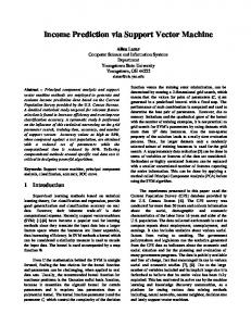
3. Fundamentals of the One-Class Centered Quarter-Sphere SVM In this paper, we exploit the one-class centered quartersphere SVM of Laskov et al. [6] to build the normal model of sensor measurements in a sliding time window. They have converted the quadratic optimization problem of the one-class SVM to a linear optimization problem. The geometry of the one-class centered quarter-sphere SVMbased approach is shown in Figure 1.

Feature 2

Margin Support vectors (0 < a < 1/vm) Non Support vectors (a = 0)

R

Non-Margin Support vectors (Outliers) (a = 1/vm)

Origin

Feature 1

Figure 1. Geometry of the quarter-sphere formulation of one-class SVM The constrained optimization problem of the one-class centered quarter-sphere SVM is formalized as follows: min

R,ξm

R2 +

1 υm

m 

ξi

(1)

i=1

subject to : φ(xi )2 ≤ R2 + ξi , ξi ≥ 0, i = 1, 2, . . . m where m denotes the number of data vectors in the training set. The parameter υ  (0, 1) controls the number of outliers. The squared norm φ(xi )2 is given by the dot product φ(xi )·φ(xi ), which indicates a measure of similarity between φ(xi ) and φ(xi ) in the feature space. A kernel function k(xi , xi ) is used to compute the similarity of any of two vectors in the feature space using the original attribute set. Hence, the dual formulation of (1) will become: minm

α

subject to :

m  i=1

−

m 

αi k(xi , xi )

(2)

i=1

αi = 1, 0 ≤ αi ≤

1 , i = 1, 2, . . . m υm

where αi is the Lagrangian multiplier. In order to fix the center of the quarter-sphere at the origin, the mapped data vectors in the feature space need to be subtracted from the m  1 φ(xi ). The centered kernel matrix Kc can mean μ = m i=1

991

be obtained in terms of the kernel matrix K = k(xi , xj ) = (φ(xi ) · φ(xj )) using Kc = K − 1m K − K1m + 1m K1m , 1 . where 1m is an m × m matrix with all values equal to m From equation (2), the {αi } value can be easily obtained using some effective linear optimization techniques [9]. The data vectors in the training set can be classified depending on the results of {αi }, as shown in Figure 1. The training 1 , which fall on the quarterdata vectors with 0 ≤ α ≤ υm sphere, are called margin support vectors. Their distances to the origin indicate the minimal radius R of the quartersphere and can be used to determine any new unseen data vector as normal or anomalous.

N(S0) S1 S2

S6

S0 S3

S5 S4

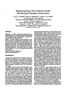
Figure 2. Example of a closed neighborhood N (S0 ) of the sensor node S0

4. Adaptive and Online Outlier Detection Techniques for Wireless Sensor Networks

Each data vector is composed of multiple attributes xil j, i d : j = 0 . . . k, l = 1 . . . d} and x   . where xij = {xil j j At time t, S0 has collected its m measurements from time , . . . , xt−1 t − m to time t − 1: {xt−m 0 0 }. Our aim is to online identify every new measurement collected by S0 as normal or anomalous. This local process can be applied to each node in the network and thus scales well to large WSNs.

In this section, we will describe our three online and local outlier detection techniques, which take different strategies to sequentially update the normal model formed by the oneclass centered quarter-sphere SVM. The policies concerning updating the normal model in these techniques include updating (i) at each time interval, (ii) at a fixed-size time window, and (iii) depending on the previous decision results. These proposed techniques enable each sensor node in the network to exploit temporal correlations among its most recent sensor measurements to identify its new arriving measurement as normal or anomalous in real-time. Moreover, using the high degree spatial correlations that exist between sensor readings of adjacent nodes, each node has more information to verify local outliers they detected. The whole detection process does not only depend on a node’s own decision criterion learned from its temporal readings but also on the decision criteria learned from its spatially neighboring nodes.

4.2. Instant Outlier Detection Technique The simplest method of updating the normal model over time is to compute the minimal radius of one-class quartersphere for each training set, i.e., at each time interval. Initially, each node learns the local radius of the quartersphere using its m sequential sensor measurements, which may include some anomalous data. The one-class quartersphere SVM can efficiently find a minimal radius R to enclose the majority of these mapped sensor measurements in the feature space. Each node then locally broadcasts the learned radius information to its spatially neighboring nodes. When receiving the radius from all of its neighbors, each node computes a median radius Rm of its neighboring nodes. We use median because in estimating the ”center” of a sample set, the median is more robust than the mean. Sensor data of adjacent nodes in a densely deployed WSN tend to be spatially and temporally correlated [10]. When a new sensor measurement xt0 is collected at time t, S0 first compares the distance of xt0 from the origin with the radius R learned with respect to its m previous measurements , . . . , xt−1 {xt−m 0 0 } in a sliding window. For computation of distance between xt0 and the origin in the feature space, i.e., d(x) please refer to [3]. The data xt0 will be classified as normal if d(x) R, xt0 is a potential (temporal) outlier. In this case, S0 further compares d(x) with the median radius Rm of its neighboring nodes. If d(x) > Rm , xt0 will finally be classified as outlier in the subset N (S0 ). Thus, the decision function can be formulated as (3), where the sensor measurements with a negative value are classified as outlier.

4.1. Problem Statement We consider that sensor nodes are time synchronized and are densely deployed in a homogeneous WSN, where sensor data tends to be correlated in both time and space. The network topology is modelled as an undirected graph G where G = (S, E). S represents the nodes in the network and E represents an edge which connects two nodes if they are within radio transmission range of each other. A subset N (S0 ) represents a closed neighborhood of a node S0  S, which contains the node S0 and its k spatially neighboring nodes. The k spatially neighboring nodes are represented by Sj = {Sj : j = 1 . . . k}, i.e., N (S0 ) = {Sj  S|(Sj , S0 )  E} ∪ {S0 }. An example of N (S0 ) is the closed disk centered at S0 with the radio transmission range of S0 , as shown in Figure 2. At every time interval Δi , each sensor node in the set N (S0 ) measures a data vector. Let xi0 , xi1 , xi2 , . . . , xik denote the data vector measured at S0 , S1 , S2 , . . . , Sk , respectively. 992

f (x) = sgn(R − d(x)) ∧ sgn(Rm − d(x))

4.3. Fixed-size Time Window-based Outlier Detection Technique

(3)

The two radii R and Rm are important decision criteria for local outlier identification. Using the radius information from adjacent nodes is also to overcome the main shortcoming of unsupervised techniques, which is suffering from high false alarm rate if the given data contains many anomalies [1]. The next step of this technique is to update the normal model at each time interval. Each update step needs to add a current measurement and to remove the oldest measurement from the sliding window. This procedure is repeated with evolving the training set of fixed size. This instant outlier detection (IOD) technique is shown in Figure 3 and Table 1. m {xt-m… xt-1 }

A slightly modified version of the IOD is to identify each sensor measurement upon being collected but update the normal model at a fixed-size time window. It means that the training set will be freezed for the next n (n  m) measurements, while each new measurement upon arrival will be classified as normal or anomalous. Therefore, there is no delay in outlier detection itself. Each update step in this technique requires to add the previous n sensor measurements and to remove the oldest n measurements from the sliding window. The corresponding modification of this fixed-sized time window-based outlier detection (FTWOD) technique is shown in Figure 4 and Table 2. In fact, the FTWOD becomes like the IOD when using n = 1.

Current time (t) Time

xt-m-1

m {xt-m… xt-1 }

xt

n Current time (t+n-1) Time

Figure 3. Principle of the IOD. Circles represent sensor measurements. The ”sliding” training set is composed of the last m measurements. The black dot represents the measurement identified at current time t.

xt-m-1

xt+n-1

Figure 4. Principle of the FTWOD. The training set is updated at each n measurements.

1 procedure LearningSVM() 2 each node collects m sensor measurements for learning its own radius R and locally broadcasts the radius to its spatially neighboring nodes; 3 each node then computes Rm ; 4 initiate OutlierDetectionProcess(R, Rm ); 5 return;

. . .... 14 14’ . . ....

If (t % n == 0) initiate UpdatingProcess(xt−n+1 . . . xt );

Table 2. The modification for the FTWOD.

6 procedure OutlierDetectionProcess(R, Rm ) 7 when xt arrives 8 compute d(x); 9 if (d(x) > R AND d(x) > Rm ) 10 xt indicates an outlier; 11 else 12 xt indicates a normal measurement; 13 endif; 14 initiate UpdatingProcess(xt ); 15 set t ← t + 1; 16 return;

4.4. Adaptive Outlier Detection Technique The policies of the above two techniques is updating the normal model either at each time interval or at n time intervals, without considering the impact when a normal or anomalous measurement is incorporated into the sliding training set. Moreover, they introduce a high communication load due to the fact that each node is required to locally broadcast the updated R to its neighboring nodes. Thus, for the sake of energy efficiency and computational simplicity, we introduce a third technique, which takes a new strategy to update the normal model depending on the previous decision results, i.e., only when a new measurement will have a significant impact on the previous normal model. As shown in Figure 1, the margin support vectors and outliers have non-zero α values so that the dual formulation of (1) will not be met if they are added into the existed training set. In order to meet the constraints of (2) and find a minimal radius, when a current measurement is detected

17 procedure UpdatingProcess(xt ) 18 update the training set: the oldest measurement xt−m is removed and replaced by xt . 19 recompute R using the updated training set. 20 locally broadcast R to its neighboring nodes; 21 recompute Rm of its neighboring nodes; 22 return;

Table 1. The pseudocode of the IOD.

Once the radius of a node is updated, the node locally broadcasts the new radius R to its neighboring nodes. The median radius Rm of neighboring nodes also needs to be recomputed. The updated R and Rm are used to identify the next sensor measurement as normal or anomalous. 993

as margin support vector or outlier, this technique adds all the previous n’ measurements including the current measurement into the training set and also removes the same amount of the oldest measurements from the training set. Due to the fact that compared to normal data, outliers and margin support vectors are very rare [1], this technique is more efficient in terms of energy and computational costs. The corresponding modification of this adaptive outlier detection (AOD) technique is shown in Figure 5 and Table 3. m {xt-m… xt -1}

its 6 spatially neighboring nodes, namely nodes 3, 4, 8, 12, 20, 14. The network recorded ambient temperature, relative humidity, soil moisture, solar radiation and watermark measurements at 2 minutes intervals. In our experiments, we use a 6am-6pm period of data recorded on 20th September 2007 with two attributes: ambient temperature and relative humidity for each sensor measurement. The data values are normalized to the range [0, 1]. The amount of anomalous data is about 10% of normal data. The labels of measurements are obtained depending on the degree of dissimilarity between one another.

n’ Current time (t+n’-1) Time

xt-m-1

xt+n’-1

Figure 5. Principle of the AOD. The black dot represents the measurement identified as a margin support vector or an outlier. . . .... 14 14’ . . ....

If (xt is an outlier or a margin support vector)  initiate UpdatingProcess(xt−n +1 . . . xt );

Figure 6. Grand-St-Bernard deployment in [2]

Table 3. The modification for the AOD.

5.2. Experimental Results and Evaluation

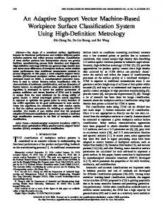
5. Experimental Results and Evaluation We have tested the following three kernel functions: (i) Linear kernel function: kLinear = (x1 .x2 ), where {x1 , x2 } are the data vectors; (ii) Radial basis function (RBF) kernel function: kRBF = exp(−x1 − x2 2 /σ 2 ), where σ is the width parameter of the kernel function; and (iii) Polynomial kernel function: kP olynomial = (x1 .x2 + 1)r , where r is the degree of the polynomial. Kernel matrices generated using the above kernel functions were centered. We have evaluated two important performance metrics, the detection rate, which represents the percentage of anomalous data that are correctly considered as outliers, and the false alarm rate, also known as false positive rate (FPR), which represents the percentage of normal data that are incorrectly considered as outliers. We have examined the effect of the regularisation parameter υ for our three outlier detection techniques and the technique presented in [3]. υ represents the fraction of outliers and we have varied it in the range from 0.01 to 0.25 in intervals of 0.03 and the kernel width parameter σ is set to 0.25. A receiver operating characteristics (ROC) curve is used to represent the trade-off between the detection rate and the false alarm rate. The larger the area under the ROC curve, the better the performance of the technique. Figure 7 shows the ROC curves obtained for the four techniques using the RBF kernel function for synthetic data. Figure 7(b) (c) show the detection rate and the false alarm

This section specifies the performance evaluation of our three techniques compared to the online outlier detection (OOD) technique presented earlier in [3]. In our experiments, we have used synthetic data as well as real data gathered from a deployment of WSN using the SensorScope System [2]. For the simulation, we use Matlab and consider a closed neighborhood as shown in Figure 2, which is centered at a node with its 6 spatially neighboring nodes.

5.1. Experimental Datasets The 2-D synthetic data used for each node is composed of a mixture of three Gaussian distribution with uniform outliers; the mean is randomly selected from (0.3, 0.35, 0.45), and the standard deviation is selected as 0.03. Subsequently, 10% (of the normal data) anomalous data is introduced and uniformly distributed in the interval [0.5, 1]. The data values are normalized to fit in the [0, 1]. The OOD in [3] identifies outliers in an online manner using the same training set without considering the evolution of the normal model over time. The testing data used for each node comprises of 200 normal and 20 anomalous data. The real data are collected from a closed neighborhood from a WSN deployed in Grand-St-Bernard as shown in Figure 6. The closed neighborhood contains the node 2 and 994

(a) ROC Curves (RBF Kernel Function)

IOD FTWOD AOD OOD

20

IOD

FTWOD AOD

AOD

80

40

OOD

10

15

20

FPR (%)

OOD

15

60

10

40

5

20

20 5

IOD

FTWOD

60

0

(c) False Alarm Rate Vs Nu (RBF Kernel Function)

FPR (%)

DR (%)

80

(b) Detection Rate Vs Nu (RBF Kernel Function)

100

DR (%)

100

0

0

0.05

0.1

0.15

Nu (v)

0.2

0.25

0

0

0.05

0.1

0.15

Nu (v)

0.2

0.25

Figure 7. (a) ROC curves with RBF kernel for synthetic data; (b) Detection rate with RBF kernel for real data; (c) False alarm rate with RBF kernel for real data.

IOD FTWOD AOD

Computational complexity Training Testing O(N ∗ L) O(N ∗ m) O((N/n) ∗ L) O(N ∗ m) O(n ∗ L) O(N ∗ m)

Memory complexity O(d ∗ m) O(d ∗ (m + n)) O(d ∗ (m + n ))

Acknowledgment This work is supported by the EU’s Seventh Framework Programme and the SENSEI project.

Table 4. Complexity analysis of three online outlier detection techniques.

References [1] V. Chandola, A. Banerjee, and V. Kumar. Outlier detection: A survey. Technical Report, University of Minnesota, 2007.

rate obtained for the four techniques using the RBF kernel function for real data. Simulation results show that our three techniques achieve better accuracy compared to the technique in [3]. It has been previously shown that work of [3] outperforms a batch outlier detection technique [7] for WSNs. Having these new protocols outperforming the work in [3], we conclude that our protocols are more efficient in detecting outliers in WSNs in an online manner. Computational and memory complexity of our techniques are presented in Table 4, where m and N devote the number of data in the training and testing sets, respectively, d represents the dimensionality of the measurements and O(L) represents the computational complexity of solving a linear optimization problem.

[2] http : //sensorscope.epf l.ch/index.php/M ainP age. [3] Y. Zhang, N. Meratnia, and P. Havinga. An online outlier detection technique for wireless sensor networks using unsupervised quarter-sphere support vector machine. ISSNIP 2008, to appear. [4] B. Scholkopf, J. C. Platt, J. C. Shawe-Taylor, A. J. Smola, and R. C. Williamson. Estimating the support of a highdimensional distribution. Neural Computation, 13(7):14431471, 2001. [5] D. M. J. Tax and R. P. W. Duin. Support vector data description. Machine Learning, 54(1):45-66, 2004. [6] P. Laskov, C. Schafer, and I. Kotenko. Intrusion detection in unlabeled data with quarter sphere support vector machines. Detection of Intrusions and Malware & Vulnerability Assessment, 2004.

6. Conclusion [7] S. Rajasegarar, C. Leckie, M. Palaniswami, and J. C. Bezdek. Quarter sphere based distributed anomaly detection in wireless sensor networks. IEEE International Conference on Communications, June 2007.

In this paper, we have developed three one-class SVMbased outlier detection techniques that update the normal model of the sensed data in an online manner. We compared the performance of these techniques with an earlier technique using synthetic and real data of the SensorScope System. Experimental results show that our techniques achieves better detection accuracy and lower false alarm, while keeping the computational complexity and memory costs low. Our future research includes testing the communication overhead of our techniques, examining the effect of the kernel parameters, and real implementation of the protocols on the sensor nodes.

[8] M. Davy, F. Desobry, A. Gretton, and C. Doncarli. An online support vector machine for abnomal events detection. Signal Processing, 8(2):52–57, 2006. [9] S. G. Nash and A. Sofer. Linear and nonlinear programming. McGrawHill, 37(3-4), 1996. [10] Y. Zhang, N. Meratnia, and P. Havinga. Outlier detection techniques for wireless sensor networks: A survey. Technical Report, University of Twente, 2007.

995