CS paradigm relies on two key properties: sparsity and incoherency. A signal. N xâ ... with quadratic constraints that solves the following problem: min .... Therefore, our method is called Adaptive Compressed Sampling (ACS). ...... of coefficients based upon the classes of the left and parent regions was done in [ 40].
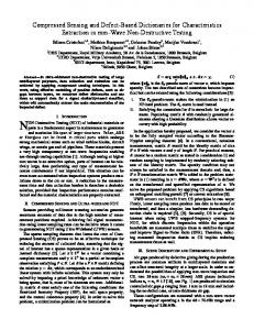
Adaptive Compressed Image Sensing Using Dictionaries Amir Averbuch*, Shai Dekel** and Shay Deutsch* Abstract. In recent years, the theory of Compressed Sensing has emerged as an alternative for the Shannon sampling theorem, suggesting that compressible signals can be reconstructed from far fewer samples than required by the Shannon sampling theorem. In fact the theory advocates that non-adaptive, ‘random’ functionals are in some sense optimal for this task. However, in practice Compressed Sensing is very difficult to implement for large data sets, since the algorithms are exceptionally slow and have high memory consumption. In this work, we present a new alternative method for simultaneous image acquisition and compression called Adaptive Compressed Sampling. Our approach departs fundamentally from the (non adaptive) Compressed Sensing mathematical framework by replacing the ‘universal’ acquisition of incoherent measurements with a direct and fast method for adaptive transform coefficient acquisition. The main advantages of this direct approach are that no complex recovery algorithm is in fact needed and that it allows more control over the compressed image quality, in particular, the sharpness of edges. Our experimental results show that our adaptive algorithms perform better than existing non-adaptive methods in terms of image quality and speed.
* Tel-Aviv University ** GE Healthcare and Tel-Aviv University
1
1 Introduction Equation Section 1 The Shannon sampling theory is at the core of nearly all signal acquisition protocols. The classic Shannon Theorem states that the sampling rate, i.e. the Nyquist rate, must be at least twice the maximum frequency present in the signal (see e.g. [48]). However, the Nyquist rate is too high and results in a massive data acquisition that must be compressed in order to be either stored or transmitted. In addition, there are important and emerging applications in which high sampling rates are very expensive or limited by physical or physiological constraints. In recent years, a novel approach for signals sampling, known as Compressed Sensing (CS) [1,9,10,11, 35] has emerged. CS is an alternative to the Nyquist rate for the acquisition of ‘sparse’ signals. Instead of uniformly sampling the signal at Nyquist rate, in the CS theory one is given a budget of n independent ‘questions’ to ask about the signal x N , with n N . These questions take the form of n fixed linear functional i , , asking for the values yi i , x , 1 i n . The vectors i N form the sensing matrix
(1 , 2 ,..., n ) , such that y x , where the dimension of is n N . In the next stage, a numerical optimization method is used to reconstruct the full-length signal from the small amount of collected data. The CS paradigm relies on two key properties: sparsity and incoherency. A signal x N is k -sparse if there exists a transform basis [ 1 , 2 ,..., N ] in which the number of
‘significant’ coefficients i x, i is relatively small k N . The basis can be, for example, a wavelet basis [31], Fourier basis [48], or a local Fourier basis [48], depending on the application. There are also the tight frames such as Curvelets [18] or Contourlets [57] that incorporate directional information, thereby allowing a sparser representation of curve singularities. Incoherency, which is concerned with the acquisition modality, states that the sensing waveforms should have an extremely dense representation in . Based on these two properties, one can design sampling protocols that capture useful information content embedded in a sparse signal and condense it into small data amount. A related condition to incoherency, which also proved to be very useful in studying the general robustness of CS, is the so-called Restricted Isometry Property (RIP) [16]. Given a measurement matrix (and a basis ), the RIP can provide a sufficient condition for a stable solution for both k -sparse and compressible (in the basis ) signals. In other words, the matrix preserves the information in a sparse or compressible signal if it satisfies the RIP condition. In general, constructing a measurement matrix that satisfies the RIP condition for large k and N is a hard combinatorial problem [52]. However, the RIP condition can be achieved for a large class of randomized matrices with a high probability [11, 36]. In scenarios where there is no noise present, the recovery of an unknown signal x from the measurements vector y would ideally be achieved by searching for the l0 –sparsest representation that agrees with the measurements (1.1) ˆ arg min 0 subject to y 1 . If the key properties of sparsity and incoherency are realized by and , then only n 2k measurements are needed to recover a k -sparse signal via l0 minimization [25]. Unfortunately, the l0 minimization problem leads to a daunting NP-complete combinatorial optimization problem [52]. Instead of solving the l0 minimization problem, non-adaptive CS theory seeks to solve the ‘closest possible’ tractable minimization problem, i.e. the l1 -minimization
2
ˆ arg min
1
subject to y 1 .
(1.2)
This modification, known as basis pursuit [21], leads to a much simpler convex problem, which approximates the original problem and can be solved by various classical optimization techniques. But at the same time, minimizing the l1 norm finds a sparse approximation because it prevents diffusing the energy of the signal over a large number of coefficients. It typically requires a number of n O (k log( N / k ) measurements to robustly recover k -sparse and compressible signals. One can adjust (1.2) to deal with cases where x or y are corrupted with additive noise, by replacing the equality y 1 , by an approximation constraint [21], [17]. Another such algorithm, which is more suitable for sparse and smooth images, is the minimization of the total variation with quadratic constraints that solves the following problem: min x x
TV
subjectto x y ,
(1.3)
where
x TV i , j ( x(i 1, j ) x(i, j )) 2 ( x(i, j 1) x(i, j )) 2 , is the total variation and depends on the noise level. In general, solving the total variation problem (1.3) provides a better image quality for image reconstruction at the expense of greater time complexity. Although different convex optimization algorithms such as basis pursuit are optimal in the sense that they provide a global minimum, they involve expensive computations when applied to large scale signals. Therefore a second approach, using suboptimal iterative greedy methods have been proposed. Examples include matching pursuit [38], orthogonal matching pursuit [69], tree matching pursuit (TMP) [45], StOPM [37], iterative hard thresholding pursuit IHT [5], Subspace Pursuit [30], and CoSaMP [53]. Let us focus on what is one of the most promising implications of CS derivatives: the enabling and the design of new types of Compressed Imaging (CI). The potential of a dramatic reduction in sampling rates, power consumption, and computational complexity is very promising for imaging applications due to its large and high dimensional datasets. One such device, which implements optical compressed sensing, is the singlepixel camera [67] inspiring a wide interest in CI applications. The single-pixel camera relies on the use of a Digital Micro-mirror Device (DMD), which is composed of a grid of mirrors, where each mirror of the array is suspended above an individual SRAM cell (see Section 4). We also note that there are experimental CI algorithms, designed for measurements taken in the frequency domain in medical imaging [47]. However, the design of an efficient and optimal measurement basis in such a system is still a challenging problem. Although theoretically very powerful, there is still a huge gap between the CS theory and imaging applications. We note few of these key difficulties: 1.
Lack of control on the output of the compressed image. From the theory of wavelet approximation, it is clear that the error of n -term wavelet approximation is characterized by the ‘weak-type smoothness’ of the image as a function in a Besov space [34]. In terms of image representation, more wavelet coefficients are needed to achieve a specified level of quality if the image contains higher visual activity such as edges and texture parts. However, the existing CS architecture is not adaptive and the number of measurements is determined before the acquisition process begins with no feedback during the acquisition process on the improved quality. 2. Computationally intensive sampling process. Constructing an efficient and fast sampling operator for non adaptive CS remains a challenging problem. On the one hand the CS theory shows that random
3
measurement (i.e. unstructured) systems are in some sense an optimal strategy for acquiring sparse signals. However, sampling operators of random binary patterns are in nature dense matrices that require huge memory allocations and intensive computations for large values of N and n . It is impractical even for an image of size 256 256 . Some of these practical challenges have already been somewhat addressed. The Scrambled Fourier Ensemble [14] was proposed for an MRI application and is often employed in CS research because of its fast implementation. However, the Scrambled Fourier ensemble matrices are dense and therefore still require huge memory and a significant implementation cost. Other researchers [4] developed binary sparse measurement matrices with low complexity and near optimal performance. However, these operators are only incoherent with identity matrices. The Block Hadamard Ensemble [41] was designed to offer a practical measurement operator for implementations. However, despite its good performance, it does not hold the incoherency which Gaussian or Bernoulli measurements operators hold, i.e. where the number of measurements needed for the reconstruction is near optimal. 3. Computationally intensive reconstruction algorithm. Although the algorithms designed to solve the l1 minimization (1.2) are proven to be theoretically efficient, .i.e., with polynomial complexity bounds, whenever the problem has a large scale, it requires heavy computations. The cost of each iteration (e.g. solving a linear system) increases very fast as the problem becomes larger.
In this work, we introduce an architecture that aims to overcome the drawbacks of the existing CS approach and achieve the following design goals: 1. Near minimal number of measurements. An acquisition process that captures n measurements with n N and n O k , where N is the dimension of the full high-resolution image which is assumed to be ‘ k -sparse’. 2.
Adaptivity to the image content. An acquisition process that adaptively takes more measurements if needed to achieve some compressed image target quality.
3.
A fast and efficient computational framework. The algorithm replaces the computational intensive CS recovery algorithm by a decoding process that is not more computationally intensive than the existing algorithms in use today such as in JPEG or JPEG2000 decoding.
The algorithms described in this paper were inspired by the CS idea of a sensing process that acquires a relatively small number of samples from which a sparse signal can be reconstructed. However, they depart fundamentally from the classic (non-adaptive) CS mathematical framework. Instead of acquiring the visual data using functionals that are random in nature and incoherent with the sparse basis, e.g., wavelets, we suggest a simple, direct adaptive and fast method for the acquisition of transform coefficients. We show that it is possible to use devices such as the DMD array in a single-pixel camera for the computation of arbitrary transform coefficients, where the computation of each coefficient requires a fixed number of measurements (see chapter 4). With this tool in hand, instead of asking n ‘universal’, non-adaptive questions about the signal in a form of linear functionals, our method takes linear measurements, directly in a sparse and structured basis, with each measurement based on the previous measurements. This allows us to take advantage of the geometric structure of the sparse representation explicitly, such as imposing the modeling of wavelet tree-structures over image edges to gather its significant information. The sampling process is initialized by acquiring a very small number of ‘low resolution’ measurements. Then, based on this initial data, by utilizing specific properties of the wavelet structure, our algorithm 4
adaptively extracts the significant information by using a near minimal number of measurements n N , n O ( k ) . This significant information, i.e., wavelet coefficients which correspond to image edges, is gathered based only on the subset of wavelet coefficients that were previously sampled and on an established set of rules. Therefore, our method is called Adaptive Compressed Sampling (ACS). Since the ACS algorithm takes only linear sampling directly in the wavelet domain, the computationally intensive CS recovery process from ‘pseudo-random’ measurements is avoided. As a result, the algorithm is very fast and achieves the above design goals. The outline of the paper is as follows: In Section 2 we recall the basic properties of Wavelets. In Section 3 we provide the ACS version of an exact reconstruction result for cartoon images using a scheme that samples in the wavelet domain. Using basic tools from differential geometry, we prove that our ACS scheme samples ‘efficiently’ all the non-zero wavelet coefficients of cartoon images, which correspond to the edges, thereby providing exact recovery with an ‘optimal’ number of measurements. In Section 4 we explain how we use the DMD architecture to acquire any transform coefficients in O 1 complexity. In Section 5 we review the Stat-ACS, an adaptive sampling algorithm that applies well-known statistical models of wavelet representations of images. Modeling of wavelet trees over image edges has already been used in the context of CS [45] but in a different and implicit way to speed up a reconstruction algorithm (1.2), as well as to speed up the numeric solution and to reduce the number of measurements [3]. In contrast, we use adaptively statistical tree models in a direct and explicit way, namely, at the time of the acquisition. The Stat-ACS algorithm is of higher complexity than the algorithm we presented in [33], but is more efficient in predicting significant wavelet coefficients and hence provides a better rate-distortion performance. Performance comparison results between the ACS method and the previous work demonstrate the superior performance of our ACS algorithm. Finally, in Section 6, we present a more advanced algorithm, the Tex-ACS that addresses the model of images as a mix of cartoon with local texture patches. The Tex-ACS algorithm uses a dictionary composed of local Fourier and wavelets basis functions. Experimental results presented for both the Stat-ACS and Tex-ACS, clearly show that the adaptive form of compressed sensing can provide better results in terms of higher reconstruction quality for the same number of samples.
2 The Wavelet Tree-Structure Equation Section 2 : j, k ) Recall that the univariate wavelet system (e.g. [31, 48]) is a family of real functions j ,k
2
in L2 ( ) , built by dilating and translating a unique mother wavelet function ( x )
j ,k 2 j /2 (2 j x k ) ,
(2.1)
( x)dx 0 .
(2.2)
where the mother wavelet satisfies
The perfect reconstruction property of the wavelet system is defined as f f , j ,k j ,k , j ,k
5
(2.3)
where is a dual of . For special choices of , the set j ,k forms an orthonormal basis for L2 ( ) and then, . Wavelets are usually constructed from a Multi-Resolution Analysis (MRA), which is a sequence of closed subspaces of L2 ( )
V j 0 ,
....V2 V1 V0 V1 V2 ...,
Usually, one starts the construction from a scaling function (generator) L2 equation ak 2 k .
k
In the orthonormal case, one then sets V j span j ,k : 2 j 2 2 j k : k W j : span j ,k : k
, with V
j 1
j
V j L2 ( ) .
that satisfies a two-scale
and constructs
such that
W j 1 V j . A classic example for an orthonormal system is the Haar scaling
function and wavelet:
1, x 0,1 , else. 0,
x :
1 1 x 0, 2 , 1 x : 1 x ,1 , 2 0 otherwise.
(2.4)
To obtain smooth symmetric wavelets of compact support one needs to construct Biorthogonal wavelets where . This is achieved by using a dual set of scaling functions and MRAs [31]. The wavelet model can be easily generalized to any dimension [48] via a tensor product of the wavelet and the scaling functions. Assume that the univariate wavelet and the scaling function are given. Then a bivariate separable basis is constructed using three basic wavelets
1 ( x1 , x2 ) ( x1 ) ( x2 ), 2 ( x1 , x2 ) ( x1 ) ( x2 ), 3 ( x1 , x2 ) ( x1 ) ( x2 ) . The bivariate discrete transform represents an image f ( x) L2 (
1
, , 2
3
and scaling function [31]
f k 2 u j0 ,k j0 ,k j j
0
e 1,2,3
2
) in terms of the three wavelet functions
k
2
wej ,k ej ,k ,
(2.5)
where u j0 ,k and w ej,k are coefficients. The wavelet decomposition can thus be interpreted as a signal decomposition in a set of three spatially oriented frequency subbands: LH ( e 1 ) detects horizontal edges; HL ( e 2 ) detects vertical edges and HH ( e 3 ) detects diagonal edges. A wavelet coefficient wej,k at a scale j represents the information about the image in the spatial region in the neighborhood of 2 j k ,k
2
. At the next finer scale j 1 , the information about this region is represented
6
by four wavelet coefficients, which are described as the children of wej,k . This leads to a natural tree structure organized in a quad tree structure of each of the 3 subbands as shown in Figure 2.1. Note that for each finer scale, the coefficients represent a smaller spatial area of the image at higher frequencies. As j decreases, the child coefficients add finer and finer details into the spatial regions occupied by their ancestors.
Figure 2.1: Wavelet coefficients tree structure across the subbands (MRA decomposition) Wavelet representations are considered very efficient for image compression: the edges constitute a small portion of a typical image, and a wavelet coefficient is large only if edges are present within the support of the wavelet. Consequently, the image can be approximated well using a few large wavelet coefficients. A significant statistical structure also follows: large/small values of wavelet coefficients tend to propagate through the scales of the quad trees. This property, called the persistency property, or the propagation property, has been utilized with great success in image coders [61, 65]. As an example, a sparse wavelet representation of the image ‘Lena’ and a compressed version of this image are shown in Figure 2.2, where the compression algorithm was based on the sparse representation. The Figure clearly depicts that the significant wavelet coefficients (coefficients with relatively large absolute value) are located on strong edges of the image.
(a) Sparse wavelet representation
(b) Compressed image
Figure 2.2 (a) A sparse wavelet representation of an image. Black - significant coefficient, white – insignificant coefficient (b) Compressed JPEG2000 image based on the sparse representation of (a).
7
3 Exact reconstruction of cartoon images using ACS Equation Section 3 The theory of CS contains results on the ability to achieve exact recovery of a sparse signal from a limited number of linear measurements [11, 16, 35]. In this section we present a simple theoretical result on exact reconstruction via critical sampling that serves as a foundation for our ACS algorithms. We prove that if a function is a typical ‘cartoon’ image, .i.e. a piecewise constant function over domains with smooth boundaries, then it is possible to reconstruct it exactly by adaptive wavelet coefficient sampling, using an ‘optimal’ number of measurements (up to a constant). In the following a ‘sample’ is the evaluation of the given function by a linear functional, specifically a wavelet coefficient. In this section, where the given functions are not discrete, we use the traditional notation where the scales are finer as the index j is larger (which is the opposite of the usual notation in the discrete setting). Theorem 3.1 Let f x c1 c2 1 x . where the boundary is a simple closed C 2 curve. Then, there exists
J , such that if all the non-zero Haar wavelet (2.4) coefficients f , ej,k are known for j J , then all non-zero coefficients f , ej,k , j J , can be acquired by an ACS process, where for each resolution # required samples at resolution j # f , ej1,k 0 : e 1, 2,3, k
2
.
(3.1)
First we need some definitions from Differential Geometry. Definition 3.2 [44] Given three points x ( s ), y ( ), z ( ) on a curve .We define the local radius of curvature ( x ) at each point x of by
( x ) : lim r ( x, y, z ) , , s
(3.2)
where r ( x, y, z ) is the radius of the unique circle which passes through the three points x, y, z .In the case where a line passes through the points we say that r ( x, y , z ) . Assuming a natural parameterization, the curvature k(s) at a point ( s ) is 1 . (3.3) k ( s) : ''( s) ( x) The minimal local radius of curvature of the curve is
( ) : min x x .
(3.4)
Definition 3.3 [Global radius of curvature] Given a simple closed C 2 curve . We define the global radius of curvature G ( x) at each point x of by
G ( x) min y , z r ( x, y, z ) .
8
(3.5)
The global radius of curvature of a curve is
G ( ) : min x G ( x) .
(3.6)
It is clear that the global radius of curvature is bounded by the local radius of a curvature, i.e.
0 G ( x ) ( x )x .
(3.7)
In Figure 3.1 we see an example that shows the difference between the global radius of a curvature and the local radius of the curvature. In contrast to a local radius of a curvature, the global radius of the curvature contains information about non-local parts of the curve.
Figure 3.1: Global radius of a curvature (left circle) and local radius of curvature (right circle). Let be a domain with a simple and closed C 2 boundary . Assume that the boundary is given in a the natural parametric form by ( s ) ( x( s ), y ( s ))s [0, L] , (3.8) where L is the length of the curve,
''( s) and
max ''( s) M ,
(3.9)
0 s L
0 G ( ) M G .
Let Q j ,k denote a dyadic square in
2
(3.10)
(recall that in this section, the scales are finer as j )
k (k 1) k (k 1) Q j ,k : 1j , 1 j 2j , 2 j , j , k (k1 , k2 ) 2 2 2 2
2
.
(3.11)
Lemma 3.4 Let be a smooth, closed and simple curve. If for j 2 j G ( ) ,
then, the circumscribed circle O j ,k of any cube Q j ,k , k curve .
9
2
(3.12)
contains at most one connectivity component of the
Proof: Since is a non self intersecting curve, we have G ( ) 0 . Assume, in contrast, that O j ,k contains two connected components of , 1 |[ s1 , s2 ] and 2 |[ s3 , s4 ] , with s1 s2 s3 s4 . Thus, the radius R of the circle passing through ( s1 ), ( s2 ) and ( s3 ) satisfies
G ( ) R
2 j 2 2 j , 2
(3.13)
which contradicts (3.12). We conclude that O j ,k contains only one connected component of . Thus, we may assume that if j satisfies (3.12), then either
O j ,k or has a single connectivity
component in O j ,k . Let us assume now the second case where
O j ,k has a single nonempty component and
let the entry point and exit points of in O j ,k be ( s1 ) and ( s2 ) , respectively. Define the following line:
( s) ( s1 ) ( s s1 ) '( s1 ) .
(3.14)
Lemma 3.5 If j satisfies for 1 2 2 M 2 j ,
(3.15)
with M given in (3.9), then the distance between and the segment ,(with ( s ) ( x( s ), y ( s )) given in (3.14) obeys 2 j , s s1 , s2 . (3.16) d ( ( s), )
Proof: Since 2M 2 j , the radius of curvature of is bigger than the radius of O j ,k . Therefore, the maximal length of the single connected curve segment contained in O j ,k is bounded by the circumference of O j ,k length
O j ,k s2 s1 2 2 j .
(3.17)
Using the differentiability properties of s x s , y s we obtain
x( s) x( s) x '' s s1 2 , y ( s) y ( s) y '' ( s s1 )2 Applying (3.15) and (3.17) for the parametric distance ( s) ( s) yields
10
s [ s1 , s2 ] .
( s) ( s) ( x( s) x( s)) 2 ( y ( s) y ( s)) 2 M ( s2 s1 ) 2 M 2 M 2 2
2 j
2 j
2 2 j
2
.
Since the geometrical distance is always smaller than the parametric distance, we obtain (3.16). Let j be a sufficiently fine (large) scale which obeys (3.12) and (3.15) for 16 . As depicted in Figure 3.2, let I be the strip composed from two linear segments and , that are parallel to and obtained by shifts of by 2 J 16 and 2 J 16 , respectively, in the direction of the normal of . By construction of ,
and by (3.16), the curve is confined to the strip I in Q j ,k . Define the width of I , w( I ) , to be the Hausdorff distance between and . Obviously, by construction w( I ) 2 J / 8 . Recall that f x c1 c2 1 x . For i 1,.., 4 , let Si area (Qi
(3.18)
) , where Qi
4
i 1
are the four quadrants of
Q j ,k , i.e. the four dyadic cubes at level j 1 that are contained in Q j ,k . Also, let S ( I ) area I
Q j ,k .
In Figure 3.2, we see an example of a curve component which is contained in a dyadic cube Q j ,k and is bounded by a strip I . Our proof rests on the fact that we can make the width of the strip I , to be relatively sufficiently small, such that the equality S1 S2 S3 S4 cannot hold.
Q1
Q2
Q3
Q4 I
Figure 3.2 A curve component bounded by the strip I in Q j ,k .
11
Lemma 3.6 Assume that j satisfies (3.15) for 16 . The equality S1 S2 S3 S4 holds for Q j ,k only if
Si 0, i 1, 2,3, 4 ,
(3.19)
or
22 j Si , 4
i 1, 2,3, 4 .
(3.20)
Proof. Denote the center of Q j ,k by o . If o ( I )C then does not intersect with at least one of the quadrants Qi and therefore S1 S2 S3 S4 can only hold if Q j ,k
corresponding to (3.19) or Q j ,k
c ,
corresponding to (3.20). Otherwise o I (as depicted in Figure 3.2). By (3.18)
S ( I ) w( I ) 2 side(Q j ,k )
2 j 2 2 j 2 2 j 2 . 8 8
From a simple combinatorial argument, there exists a quadrant Qi for which the intersection with I is equal or smaller than a quarter of S ( I )
I)
S (Qi
2 2 j 2 32
(3.21)
Without loss of generality, assume that (3.21) holds for i 1 and that S1 0 . This implies that
S1 S (Q1 ) S (Q1
I)
22 J 222 J 6 22 J . 4 32 32
(3.22)
On the other hand, for at least one of the other quadrants, Qi , i 2,3,4 ,
Si S (Qi
I)
2 2 J 2 . 32
(3.23)
Thus, Si S1 for one of i 2,3,4 and therefore, o I is not possible. This completes the proof of the lemma. Proof of Theorem 3.1 Let f x c1 c2 1 x , and . Let Q j ,k be a dyadic cube. If Q j ,k wej ,k f , ej ,k 0 , for e 1,2,3 . We claim that if Q j ,k
, then
, then for sufficiently large j it is impossible
that w1j ,k w2j ,k w3j ,k 0 , simultaneously. Indeed, let QJ ,k be a dyadic cube such that the scale J satisfies for
16 :
J max 0, log 2 (2 2 M ) , log 2 G ( ) .
12
(3.24)
and that w1j ,k w2j ,k w3j ,k 0 . Observe that using the notation
Assume, by contradiction that Q j ,k where the scales are finer as j
2 k1 1 2 k2 1 2 k1 1 2 k2 1/2 0, 2 f ( x , y ) dxdy f ( x , y ) dxdy j 2 j k j j 2 k2 2 k1 2 k2 1/2 1 j j j j 2 k 1/2 2 k 1 2 k 1 2 k 1 1 2 1 2 0, 2 j f ( x , y ) dxdy f ( x , y ) dxdy j 2 j k j j 2 k2 2 k1 1/2 2 k2 1 j
1 j ,( k1 ,k2 )
w
w2j ,( k1 ,k2 )
w
3 j ,( k1 ,k2 )
j
j
j
j
2 2 j
j
k1 1/2 2 j k2 1/2
2 j k1
2 j k1 1
f ( x, y )dxdy
2 j k1 1/2 2 j k2 1
2
j
k1
2
j
f ( x, y )dxdy
2 j k1 1 2 j k2 1/2
f ( x , y )dxdy
k2 1/2
(3.26)
2 j k2 1
2 j k1 1/2 2 j k2 1/2
2 j k2
(3.25)
2 j k1 1/2
2 j k2
f ( x , y )dxdy 0.
(3.27)
With the notation of Si i 1 given above, the solution of equations (3.25)- (3.27) is obtained by solving the linear algebraic system S1 1 1 1 1 S2 c2 1 1 1 1 0 . (3.28) S 3 1 1 1 1 S4 Since we may assume c2 0 , we obtain the set of solutions 4
S1 S2 S3 S4 .
(3.29)
As J satisfies (3.24) for 16 , by Lemma 3.6 we obtain that (3.29) is satified only if (3.19) or (3.20) hold. But this is a contradiction to our assumption that QJ ,k . The proof of the theorem can now be completed by a simple induction: at any resolution j J assume
we have all non-zero wavelet coefficients w ej,k . For any such non-zero coefficient wej,k , we sample the 12 wavelet coefficients
w
e j 1,l
| e 1, 2,3 , l (2k1 , 2k2 ),(2k1 1, 2k 2 ),(2k1 , 2k 2 1),(2k1 1, 2k 2 1) .
If for the cube Q j 1,l , we have wej1,l 0 for e 1, 2,3 , then we know Q j 1,l and therefore we don’t sample any wavelet coefficients supported in this cube. Otherwise our ACS process continues to sample wavelet coefficients in Q j 1,l .
13
We conclude this section by noting that Theorem 3.1 can be easily extended to a more general case where the cartoon function is a piecewise constant over a finite collection of disjoint domains with simple and closed smooth boundaries.
4 Direct sampling of transform coefficients using digital micro-mirror arrays Equation Section 4 Today’s digital camera devices are in the mega pixel range thanks to the introduction of Charged Coupled Devices (CCDs) and Complementary Metal Oxide Semiconductor (CMOS) digital technology. Assume x is a digital image consisting of N pixels that we wish to acquire. Some digital cameras perform the acquisition using an array of N CCDs after exposure to the optical image. The charges on its pixels are read row by row, fed to an amplifier and then undergo an analog-to-digital conversion. CMOS allows today’s professional cameras to acquire about 12 million pixels ( 3000 4000 ). Once the digital image x has been acquired, it is usually compressed using standard compression algorithms such as JPEG and JPEG2000. In most digital cameras, the user has the capability to control the compression/quality tradeoff through the compression algorithm. We now describe the ‘single-pixel’ camera of [67] which is used to implement a CI system as depicted in Figure 4.1.
Figure 4.1. The architecture of the CS digital camera in [67]
The ‘single-pixel’ camera replaces the CCD and CMOS acquisition technologies by a Digital Micro-mirror Device (DMD). The DMD consists of an array of electrostatically actuated micro-mirrors where each mirror of the array is suspended above an individual SRAM cell. Each mirror rotates about a hinge and can be positioned in one of two states: +12 or −12 from horizontal. Using lenses all the reflections from the micro-mirrors at a given state, (e.g., the light reflected by mirrors in +12 degree state) are focused and collected by a single photodiode to yield an absolute voltage. The output of the photodiode is amplified through an op-amp circuit and then digitized by a 12-bit analog-to-digital converter. This value should be interpreted as 14
N
v xi 1i 12 DC offset , i 1
where x x1 , , xN is a digital image, the indicator function 1i 12 obtains the value 1 if the i -th micromirror is at the state +12 and 0 otherwise and the DC offset is the value outputted when all the micro-mirrors are set to -12. In [67], the rows of the CS sampling matrix are in fact a sequence of n pseudo-random binary masks, where each mask is actually a ‘scrambled’ configuration of the DMD array (see also [2]). Thus, the measurement vector y , is composed of inner-products of the digital image x with pseudo-random masks. As we see in Figure 4.1, the measurements are collected into a compressed bitstream with possible lossy or lossless compression applied to the elements of y . At the core of the decoding process, that takes place at the viewing device, there is the minimization algorithm (1.2). Once a solution is computed, one obtains from it an approximate ‘reconstructed’ image by applying the transform 1 to the coefficients. In [67], the authors choose the transform to be a wavelet transform, but their sampling process has a ‘universal’ property. This means that any transform T , which is in incoherence with a process of pseudo-random masks (almost all reasonable transforms have this property) and in which the image has a sparse representation, will lead to a reconstruction with good approximation to the original image. Recall that our proposed approach, although inspired by the CS concept of acquisition processes of simultaneous sensing and compression of the image, departs fundamentally in the mathematical framework. Instead of acquiring the visual data using a representation that is incoherent with wavelets, we sample directly in the wavelet domain. At a glance, this might seem to be a paradox, since computing the fast wavelet transform of an N pixel image requires O N computations, whereas we want to take only n measurements with
n N . Furthermore, computing even one low-frequency wavelet coefficient requires calculating an integral over a significant portion of the image pixels, which requires O N computations. This ‘paradox’ is solved by using the Single-Pixel Camera in a different way than in [67]. There exist DMD arrays with the functionality that a micro-mirror can produce a grayscale value not just 0 or 1 (contemporary DMD can produce 1024 grayscale values). One can use these devices to compute arbitrary real-valued functional acting on the data, since any functional g can be represented as a difference of two ‘positive’ g , g functionals, such that g g g ,g , g 0 . This allows us to compute any transform coefficient using only two measurements. Also, we may leverage onthe ‘feedback’ architecture of the DMD and make decisions on future measurements based on existing value measurements. As we shall see, this adaptive sampling process relies on a well-known modeling of image edges using a wavelet coefficient tree-structure. Then, decisions on which wavelet coefficients should be sampled next are based on the values of the wavelet coefficients obtained so far. Let us now give the example of the acquisition of an arbitrary Haar wavelet coefficient, that can be computed by using even the simpler binary DMD using only two measurements. The wavelet coefficient associated with a Haar wavelet in subband e 1 is given by 2 k1 1 2 2jk 1 j
f ,
1 j ,k
j
2 j k2 1 2
f x1 , x2 dx1dx2
j
2 j k1 1 2 j k2 1
j
2 k2
2 k1
2 k2 1 2 j
f x1 , x2 dx1dx2 .
(4.1)
This implies that for the purpose of computing a wavelet coefficient of the first type using a binary DMD array, we need to rotate and collect twice, into the photodiode, responses from two subsets of micro-mirrors, each 15
supported over neighboring rectangular regions corresponding to the scale j and location k . From (4.1), the value of the wavelet coefficient we wish to acquire is the difference of these two outputs multiplied by 2 j .
5 Stat-ACS - An ACS algorithm based on statistical modeling in the wavelet Domain Equation Section 5 In [33], we presented a rather simple ACS algorithm, in which wavelet coefficients were sampled based on local Lipschitz smoothness estimates using their ancestors [22, 48]. In this work we elaborate on a more advanced statistical based ACS algorithm: the Stat-ACS. We use information-theoretic analysis tools to estimate statistical dependencies between a wavelet coefficient and related coefficients at adjacent spatial locations and scales. The information obtained from previously sampled coefficients is summarized into a ‘linear predictor’ which predicts the significance of a coefficient that has not been sampled yet. Since the StatACS algorithm operates on a relatively complex dependence network, we employ hash tables to construct efficient dynamic dictionaries. This enables the algorithm to maintain an acquisition process that captures n measurements, with n N , where N is the number of pixels and n O k , where the image is assumed to be ‘well approximated’ by k wavelet terms. While the Stat-ACS algorithm is more complex than the algorithm in [33], its scheme increases the probability that significant wavelet coefficients will not be ‘missed’ and will be sampled. Thus, the Stat-ACS algorithm suggests a trade-off between a higher complexity of the algorithm to a higher efficiency in recovering edges and important features in the image.
5.1 Wavelet statistical models Statistical modeling of images is used in tasks such as compression [8, 24, 29, 46], denoising [29, 68] and classification [23]. In most of these works, wavelet coefficients of natural images are modeled by Generalized Gaussian marginal statistics. The Probability Density Function (PDF) of the Generalized Gaussian density is defined as
p( x; , )
2(1/ )
e
( x / )
,
(5.1)
where models the width of the PDF peak, is inversely proportional to the decreasing rate of the peak and
( z ) et t z 1dt . z 0 is the Gamma function. 0
Also, these works revel that for images, wavelet coefficients are not statistically independent mainly due to the geometric properties of edge singularities. Thus, at least for natural images, there are significant dependencies between the magnitude of pairs of wavelet coefficients which correspond to adjacent spatial locations, orientation and scales. There are various statistical models which have been developed to capture the dependencies between wavelet coefficients. Image compression schemes that use spatial and scale-to-scale dependencies have proven to be extremely effective; large magnitude wavelet coefficient may indicate that the wavelet coefficient at the
16
adjacent finer scale, same subband and relative location also has a large magnitude. The conditional distribution of a coefficient, given its coarser scale ancestors, was captured by the Embedded Zero-tree Wavelet (EZW) Coder [65] to encode entire trees of insignificant coefficients with a single symbol. A predictive method was used in [61] to provide high quality zero-tree coding results. Several studies [55, 56, 58] predict blocks of fine coefficients from blocks of coarse coefficients by using vectorized lookup tables. Adaptive entropy coding was used in [63] to capture conditional statistics of coefficients that are based on the most significant bits of each of the eight spatial neighbors and the coefficients at the coarser scale. A switch between multiple probability methods that depend on the values of neighboring coefficients was done in [24]. The EZW coder was extended in [70] to use local coefficient contexts. An adaptively condition the encoding of classification maps of regions of coefficients based upon the classes of the left and parent regions was done in [40]. The hidden Markov tree model (HMT) [29] also captures the dependencies between a parent and its children. We highlight some important wavelet coefficient dependencies as illustrated in Figure 5.1. X is a wavelet coefficient, P , its parent at the coarser scale and NX is a predefined set of adjacent coefficients of X at the same subband.
Coarser scale (Level j+1)
Finer scale (Level j)
Figure 5.1. Set of conditioning candidates for a given coefficient X.
First use of mutual-information estimation to measure dependencies between wavelet coefficients appears in [46]. Recent studies have adopted the mutual information estimation for an efficient characterization of statistical dependencies in an overcomplete wavelet representation [39] and multiscale directional transforms such as counterlets [57] and curvelets [7]. Recall that the mutual information between two random variables X and Y with joint density p ( x, y ) and marginal densities p ( x ) and p ( y ) is defined in [64] to be
I ( X ; Y ) p( x, y ) log
p( x, y) dxdy . p ( x) p ( y )
(5.2)
The mutual information I ( X ; Y ) can be interpreted as the amount of information Y conveys about X and vice versa. A higher value of I ( X ; Y ) implies a stronger dependency between X and Y and thus, it is easier to estimate X from Y . In practice, the random variables are discrete and in our case the pdf of p ( x, y ) , p ( x ) , p ( y ) are unknown and must be estimated from the empirical data. Studies of this problem resort to non-
17
parametric histogram estimation of the pdf [8, 54, 66]. The histograms are usually constructed as follows: the ranges of X and Y are partitioned into N X and NY intervals, respectively. The histogram of ( X , Y ) obtained
j NY , and yields an approximation to the from the empirical data is denoted as p X ,Y (i, j ) |,for1 i N X ,1
pdf p ( x, y ) . Similarly, the marginal distributions, p ( x ) , p ( y ) are estimated. Consider a pair of wavelet coefficients X and Y . Based on the estimated discrete probability distribution, we use the following estimator for the mutual information [51]:
k k N p (i, j ) Iˆ( X ; Y ) p X ,Y (i, j ) log X ,Y ij log ij , p X (i) pY ( j ) i , j N ki k j i j
(5.3)
kij
replaces pij , where kij is the number of coefficient pairs in the joint histogram cell (i, j ) , N ki j kij and k j i kij are the marginal distribution histogram estimates. The mutual information can thus
such that
provide us with a criterion for a selection process in which energy values are extracted according to a previously-computed subset of neighbors N , whose relationship with shows the maximal mutual information across a wide range of images. Table 5.1-Table 5.3, show mutual information estimation results for a wavelet coefficient (we use the (9, 7) wavelet basis), which is modeled to be dependent on a single other coefficient. The mutual information estimates is the average of the two next to finest scale. The index (i, j ) which correspond to the coefficient NX ij refers to the location of a neighbor that is located in the j ( j 0 ) up- hand row and i ( i 0 ) left-hand column ( for i 0 or j 0 we replace up-hand and left- hand with down-hand and right-hand, respectively). For example, NX 1,0 , NX 0,1 corresponds to the up-hand and left-hand side neighbors of X . Similar results were also obtained on a variety of different images. We measured and compared the mutual information with a single neighbor (scale, location, subband). The left, Up and Parent coefficients showed the highest mutual information, where the Left coefficient is the most informative in the horizontal subband, and the Up coefficient is the most informative in the vertical and diagonal.
Iˆ - mutual information estimate Iˆ( X ; P) Iˆ( X ; NX )
Lena
Peppers
Barbara
0.109
0.12
0.08
0.07
0.05
0.08
Iˆ( X ; NX 1,0 )
0.103
0.08
0.123
Iˆ( X ; NX 1,1 )
0.09
0.05
0.095
Iˆ( X ; NX 0,1 )
0.119
0.115
0.132
Iˆ( X ; NX 0,1 )
0.1208
0.114
0.13
Iˆ( X ; NX1,1 )
0.09
0.04
0.09
1, 1
18
Iˆ( X ; NX 1,0 )
0.1
0.07
0.11
Iˆ( X ; NX1,1 )
0.07
0.12
0.07
Table 5.1: Mutual information estimate in the two next to finest horizontal subband,
Iˆ - mutual information estimate
Lena
Peppers
Barbara
Iˆ( X ; P)
0.127
0.141
0.07
Iˆ( X ; NX 1,1 )
0.088
0.05
0.1
Iˆ( X ; NX 1,0 )
0.197
0.139
0.22
Iˆ( X ; NX 1,1 )
0.106
0.07
0.11
Iˆ( X ; NX 0,1 )
0.109
0.08
0.12
Iˆ( X ; NX 0,1 )
0.107
0.08
0.125
Iˆ( X ; NX1,1 )
0.109
0.06
0.11
Iˆ( X ; NX 1,0 )
0.199 0.087
0.14 0.05
0.22 0.1
Iˆ( X ; NX1,1 )
Table 5.2: Mutual information estimate in the two next to finest vertical subband
Iˆ - mutual information estimate Iˆ( X ; P) Iˆ( X ; NX )
Lena
Peppers
Barbara
0.107
0.07
0.06
0.075
0.02
0.12
Iˆ( X ; NX 1,0 )
0.12
0.05
0.18
Iˆ( X ; NX 1,1 )
0.10
0.03
0.124
Iˆ( X ; NX 0,1 )
0.101
0.05
0.147
Iˆ( X ; NX 0,1 )
0.101
0.05
0.145
Iˆ( X ; NX1,1 )
0.108
0.03
0.125
Iˆ( X ; NX 1,0 )
0.122
0.04
0.176
Iˆ( X ; NX1,1 )
0.07
0.03
0.124
1, 1
Table 5.3: Mutual information estimate in the two next to finest diagonal subband
19
5.2 The Stat-ACS Algorithm The Linear Predictor To impose the statistics of wavelet coefficients’ strongest dependencies, exhibited by the mutual information, into the use of the Stat-ACS algorithm, we choose to utilize a linear predictor for the size of a coefficient magnitude. The linear predictor is defined as: l (Q) Q k Qk ,
(5.4)
k
where Qk correspond to the magnitudes of a subset of potential conditioning neighbors (depicted in Figure 5 .1) and the weights k used to compute the predictor are chosen to minimize the expected squared error, such that (5.5) E (QQT )1 E (C ' Q) , where E () indicates the expected value of a random variable, C ' corresponds to the coefficient magnitude being estimated and Q is a vector contains the magnitudes of the conditioned neighbors. The coefficients, we use in the conditioning set are the left-hand and up-hand side neighbors NX 0,1 , NX 1,0 , and the parent P . The weights (5.5) were determined as the average weights obtained from a number of typical images. During the processing of the Stat-ACS algorithm, we utilize the linear predictor l (Q) explicitly to estimate the absolute value of an unsampled coefficient. We now review in detail the way in which the joint statistical model is used in the framework of our Stat-ACS algorithm. We begin with preliminary notation: given an arbitrary wavelet coefficient corresponding to the index (e, j 1, (k1 , k2 )) and label ' P ' (as for ‘Parent’), its four children at the next finer resolution correspond to the indices (e, j, 2k1 , 2k2 ) , (e, j, 2k1 1, 2k2 ) , (e, j, 2k1 , 2k2 1) , (e, j, 2k1 1, 2k2 1) , where we label the indices (e, j, 2k1 , 2k2 1) and (e, j, 2k1 1, 2k2 ) as ' L ' (as for Left ) and 'U ' (as for Up), respectively. In this algorithm, the indices of the sampled coefficients found to be significant are placed in a ‘processing queue’, together with their labels ‘Parent’, ‘Left’, ‘Up’ or ‘Right’. The labels given to each coefficient refer to the relation between the input and output indices of the linear predictor: a coefficient with label ' P ' indicates that the linear predictor attempts to estimate the significance of its four children at the next higher resolution; a label of ' L ' indicates that the linear predictor attempts to estimate the right-hand neighbor of that coefficient, and a label of 'U ' indicates that the linear predictor attempts to estimate the down spatial neighbor of that coefficient. Note that a coefficient can have more than one label. The index and value of the coefficient at the head of the processing queue is passed as input to the linear predictor, l (Q) , given in (5.4) which attempts to assess whether the related unsampled coefficients are potentially significant. Once the prediction asserts that an unsampled coefficient is with high probability significant, it is sampled by the sensing apparatus. The algorithm ‘scans’ each subband such that the most informative spatial neighbor could be used in the processing queue. Thus, in the horizontal subband, where the left neighbor conveys the highest information - the rows are scanned first (left to right order), and in the vertical and diagonal subbands, the columns are scanned first (up to right order) since the up coefficient is the most informative.
20
The Hash Table Incorporating a contextual model into a Stat-ACS algorithm, that operates simultaneously on the information of several coefficients (parent, left, up neighbors), requires the use of a ‘sparse’ data structure which supports fast ‘find’ and ‘add’ operations. This is essential so as to ensure our ACS algorithm is of complexity O ( n ) , where n is the number of measurements, with n N ( N number of pixels in the image). To this end we use a Hash Table [27] that on average performs ‘find’ and ‘add’ operations in O 1 time. During the adaptive sampling process, we store in the hash table the coefficients that were sampled and we later retrieve their values for the purpose of predicting the significance of unsampled coefficients. We summarize the algorithm in the pseudocode below.
Stat-ACS Algorithm ACS based on statistical modeling in the wavelet domain 1. Acquire the values of all low-resolution coefficients up to a certain low-resolution J , each computation is completed using a fixed number of DMD array measurements as in (4.1). The initial resolution J can be selected as log2 N 2 const . In any case, J should be bigger if the image is bigger. For images of size 512 512 we used J 4 . Note that the total number of coefficients at resolutions J is 2 N , which is a small fraction of N . 2. Initialize a ‘processing queue’, P ( q ) , containing the indices of each of the wavelet coefficients at resolution J , with absolute value bigger than a given threshold Tthresh and label as a parent, ' P ' . 3. Until the queue P ( q ) is exhausted, pop out the coefficient at the head of the queue and process as follows: i) If labeled ‘P’ with index e, j, k and children coefficients have not been sampled yet a. Acquire them now. b. If the child with index e, j 1, 2k1 , 2k2 1 is significant then add its index to the head 2 1 J
ii)
of P ( q ) labeled as ‘ L ’. If in the horizontal subband and labeled ‘L’ as left of a coefficient X, find and read from the hash table the values of ‘P’, the parent of X and ‘U’, the upper neighbor of X. The values are set to zero, if coefficients are not in Hash table. Fix the input vector Q (value(' P '), value(' L '), value('U ')) for the linear predictor l (Q) . If l Q Tthresh ,then
a. Sample the group of 4 coefficients to which X belongs, i.e. have the same parent e, j, k . b. If a coefficient is significant and at resolution j 1 , add its index to the end of the queue, labeled as ‘P’. c. If the coefficient with index e, j 1,2k1 ,2k2 1 is significant, then add to the head of the queue labeled as ‘L’. (This step is similar for coefficients from the other 2 subbands) iii) Store the values of any sampled coefficient in the Hash table.
21
5.3 Stat-ACS - Experimental results A good method to evaluate the effectiveness of our approach is to benchmark it using the optimal n term wavelet approximation. It is well known [34] that for a given image with N pixels, the optimal orthonormal wavelet approximation using only n coefficients is obtained using the n largest coefficients f , ej11,k1 f , ej22,k2 f , ej33,k3 n
f f , ejii ,ki ejii ,ki i 1
L2
2
min f # n
e , j ,k
,
f , ej ,k ej ,k
. L2
2
For biorthogonal wavelets this ‘greedy’ approach gives a near-best result, i.e. within a constant factor of the optimal k -term approximation. Obviously, to find the near best n -term approximation one needs to compute all the wavelet coefficients and then select from them the n largest. Any other threshold method would also require computing each and every coefficient and testing if its absolute value is above a certain threshold. Thus, any threshold method requires order N computations, whereas our adaptive compressed sensing algorithm is output sensitive and requires only order n computations. To simulate our algorithm, we first pre-compute the entire wavelet transform of a given image. However, we strictly follow the recipe of our ACS algorithm and extract a wavelet coefficient from the pre-computed coefficient matrix only if its index was added to the adaptive sampling queue. In Figure 5.2 (a) we see a ‘benchmark’ near-best k 7000 term approximation of the image Lena using a biorthogonal (9, 7) wavelet, which achieves PSNR=31.6. In Figure 5.2 (b) we see our Stat-ACS with n 14000 and PSNR= 30.26. With n 2k , we have sampled twice as many as in the sparse representation to which we compare. In Figure 5.2 (c) and Figure 5.2 (d) we see a 5000-term and 8000-term approximations, with PSNR=29.35, and PSNR=30.1, respectively, extracted from the Stat-ACS obtained in Figure 5.2 (b). In Figure 5.3(a) and Figure 5.3 (b) we present a comparison between Figure 5.2 (a) and Figure 5.2 (d) by zooming in on specific edge results. As Figure 5.3 illustrates, the edges were recovered quite well and are comparable to the near-best 7000-term. In Figure 5.4 (a) we see a ‘benchmark’ near-best 7000-terms biorthogonal (9, 7) wavelet approximation of the Peppers image, with PSNR=30.8. In Figure 5.4 (b) we see our Stat-ACS with n 14000 and PSNR= 29.17.
22
(a)
(b) #Samples=14000, Stat-ACS
#Samples=262144, Near-best
14000-terms, PSNR=30.26
7000-terms, PSNR=31.6
(d) #Samples=14000, Stat-ACS
(c) #Samples=14000, Stat-ACS
8000-terms, PSNR=30.1
5000-terms, PSNR=29.35
Figure 5.2: Comparison of the Stat-ACS algorithm with optimal benchmark on „Lenna‟
23
(b) #Samples=14000, Stat-ACS
(a) #Samples=7000, Near-best
8000-terms, PSNR=30.1
7000-terms, PSNR=31.6
Figure 5.3: Zoom in into lenna shoulder
(b) #Samples=14000 Stat-ACS
(a) #Samples=7000 Near-best
8000-terms, PSNR=29.0
7000-terms, PSNR=30.8
Figure 5.4: Comparison of the Stat-ACS algorithm with optimal benchmark on „Peppers‟
24
5.4 Stat-ACS – Rate/distortion performance comparison to non-adaptive CS algorithms In this section we compare the performance of our Stat-ACS algorithm with some of the prominent nonadaptive CS algorithms such as the scrambled Fourier ensemble (SFE) [14] and the Scrambled Block Hadamard Ensemble (SBHE) [41]. The performances of the SFE and the SBHE have been evaluated using the following reconstruction algorithms: min-TV, l1 optimization solver, and iterative thresholding. Table 5.4 tabulates the PSNR values for three 256 256 natural images Lena, Cameraman, and Peppers. Also results from [15] are included, where random Fourier sampling matrices were applied directly in the wavelet domain. The best result for each image and each number of measurements are marked in bold letters. The results in Table 5.4 show that the imaging performance of the Stat-ACS is significantly better than all the CS algorithms.
No. Of Samples
n
[15]
l1 optimization
min-TV optimization
SFE
SFE
SBHE
10000 15000
26.5 28.7
21.5 23.9
21.1 23.7
10000 15000
26.2 28.7
20.9 23.2
20.7 23.0
10000 15000
26.7 25.3
21.6 22.7
21.4 22.6
Iterative thresholding Stat-ACS
SBHE
SFE
Lenna ( 256 256 ) 27.5 28.0 27.2 29.7 30.0 30.4 Cameraman ( 256 256 ) 27.0 27.1 26.5 29.3 29.5 29.5 Peppers ( 256 256 ) 28.6 29.0 28.1 31.2 31.7 31.2
SBHE
27.7 30.6
30.83 33.9
26.8 29.7
28.57 31.22
28.2 31.6
30.75 34.14
Table 5.4 Comparison results between various non-adaptive CS algorithms and the Stat-ACS algorithm (PSNR in dB) for 256 256 images.
5.5 Stat-ACS - Comparison to model-based compressive sensing Model based compressive sensing methods [53], [3] attempt to use wavelet representation modeling in an implicit way. The CS acquisition process is still ‘pesudo-random’, but the recovery algorithms try to integrate the assumptions on wavelet ‘structure’, with the goal of faster and more accurate recovery in the presence of noise. In this section we compare the performance of our Stat-ACS method and these methods. In Figure 5.5 we see the test image ‘Peppers’ of size N 128 128 =16384 with several recovery results of CS algorithms, all
25
using 5000 measurements. It is clear that the Stat-ACS algorithm shows results which are by far superior to the one presented in [3] both in terms of visual quality and RMSE. The key reason is that our method uses explicitly and adaptively the geometrical and statistical nature of the wavelet representation of an image. Note that the model based compressive sensing takes measurements using the random Gaussian matrices, which are universally incoherent with any sparse signal and require almost minimal number of compressive measurements to reconstruct a signal. Recall that these kind of random measurements are limited for small size images.
(a) Input Image
(b) #Samples=5000,CoSaMP (c) #Samples=5000, model-based re. RMSE=22.8 RMSE=11.1
(d) #Samples=5000, Stat-ACS RMSE=7.3807 Figure 5.5: Comparison of model based Compressive sensing and our Stat-ACS algorithm (a) Test image „Peppers‟, N 128 128 =16384 (b) Non-adaptive CS with CoSaMP (c) Non-adaptive Model Based Compressive Sensing [3] (d) Stat- ACS.
26
6 Tex-ACS - An ACS algorithm based on a
cartoon/texture model Equation Section 6 In this section we elaborate on an ACS algorithm that addresses the model of images as a mix of cartoon with local texture patches. While the edges are somewhat structured, capturing the textural parts is more difficult and elusive, though easily visually perceived. In general, texture is regarded as a function of the spatial variation in pixel intensities [20]. In the wavelet representation, the significant information of texture typically manifests at the higher frequency scales, i.e. finer resolutions with a smaller index j . The Stat-ACS algorithm of the previous section, relies on a ‘cartoon’ model of the image and is not equipped to predict significant high frequency wavelet coefficients which correspond to texture information, from the coefficients at lower resolutions. Thus, our aim is to identify the local texture areas and to sample wavelet coefficients of corresponding frequencies that are supported in these domains. We address this problem by sampling from a ‘dictionary’ composed of wavelets and local Fourierwindows components over tiles of the image. The role of the local Fourier sampling is to identify the texture information. Once we identify textural areas, we use the correlation between Fourier frequency components and wavelet coefficients with coinciding frequencies, to subsequently sample correctly the wavelet coefficients whose support overlaps these areas. In the experimental results, the suggested approach yields significant improvement in extracting the texture parts.
6.1 Texture and Wavelets in the frequency domain We very roughly sketch the properties of wavelets from a Fourier side perspective (see e.g. for more detailed analysis [31], [48]). In particular we focus on the (9, 7) CDF biorthogonal wavelet, selected by the FBI for fingerprint compression and JPEG2000 standard and also used in our experiments. Let , and , be two dual pairs of scaling functions and wavelets that generate biorthogonal wavelet bases of L2 ( ) . Recall, that the bivariate wavelet bases we use are created by a tensor product, yielding three types of dual wavelets:
1 ( x) ( x1 ) ( x2 ), 2 ( x) ( x1 ) ( x2 ), 3 ( x) ( x1 ) ( x2 ) . Denote:
ej ,k x 2 j e 2 j x k , e 1, 2,3 j ,
k
2
.
(6.1) (6.2)
In the Fourier domain the separable wavelets from (6.1) become
ˆ 1 (1 , 2 ) ˆ (1 )ˆ (2 ), ˆ 2 (1 , 2 ) ˆ (1 )ˆ (2 ), ˆ 3 (1 , 2 ) ˆ (1 )ˆ (2 ) .
(6.3)
ˆ Roughly speaking, is concentrated around the origin and ˆ away from the origin. Therefore, by (6.3),
ˆ 1 (1 , 2 ) is large at low horizontal frequencies 1 and high vertical frequencies 2 , ˆ 2 (1 , 2 ) is large at
27
high frequencies 1 and low vertical frequencies 2 and ˆ 3 (1 , 2 ) is large at high horizontal and vertical frequencies . According to the dominant frequencies computed for the wavelet in scale j 0 , one can obtain the corresponding dominant frequencies at scale j by the relation
ˆ ej ,k ( ) 2 j ˆ e (2 j ) .
(6.4)
1 ˆ ˆe f , j ,k . 2
(6.5)
Recall the Plancherel formula f , ej ,k
We wish to examine the amount of oscillatory activity exhibited in the image f over an arbitrary local area defined by a cube Q f ( x1 , x2 ), if (x, y ) Q, f Q ( x1 , x2 ) , (6.6) 0, else. Intensive oscillatory activities may indicate that the support of Q contains texture and other important features at fine scales. If the support of the wavelet coefficient ej,k , satisfies support( ej,k ) Q , then f , ej ,k fQ , ej ,k
1 ˆ ˆe fQ , j ,k , 2
(6.7)
Although the (9, 7) wavelet is not compactly supported in the frequency domain, it is ‘essentially’ supported in the frequency domain and by (6.4) its dilates have ‘peaks’ at the corresponding frequencies. Thus, if, locally, f contains corresponding frequencies, then we should expect some of the coefficients of wavelets that have essential support around that frequency to have large absolute value. In practice, we estimate the ‘energy’ of the significant local frequencies by sampling Discrete Cosine Transform (DCT) coefficients. The DCT decomposes a local block of an image over x1 , x1 N x2 , x2 N from spatial to the frequency domain N 1 N 1 1 1 fˆ (k1 , k2 ) f ( x1 n1 , x2 n2 ) cos n1 k1 cos n2 k2 . 2 2 n1 0 n2 0 N N
(6.8)
Since the DCT is a linear, real valued transform, we can compute each DCT coefficient as a combination of two ‘positive’ functionals which correspond to two DMD measurements, as in (4.1).
6.2 The Tex-ACS Algorithm For simplicity, we assume the input image to be processed is of dyadic dimensions, N1 N1 N . We subdivide the image into blocks of 16 16 pixels each, i ,l , 1 i, l N1 16 . Over each patch il , we compute using 28
(6.8), with N 16 , the three DCT coefficients fˆil (1,8), fˆil (8,1), fˆil (8,8), which correspond to the dominant frequencies of the horizontal vertical and diagonal wavelet coefficients, respectively, at scale j 2 . This implies that the algorithm is initialized by taking about 0.012 N12 local frequency samples. If any of the three DCT coefficients fˆ (k , k ), satisfies fˆ (k , k ) t , for a large threshold t , then we sample the coefficients of il
1
il
2
1
2
j
j
wavelets at the corresponding scale and subband whose support overlaps significantly the block i ,l . Also, if the frequency component fˆ (k , k ) is significant, it is also likely that significant texture information exists at il
1
2
adjacent scales. Thus in such case we sample the frequency components fˆil k1 / 2 , k2 / 2 and fˆil 2k1 , 2k2 , to test oscillatory activities in the adjacent frequency domains. If fˆil k1 / 2 , k2 / 2 t j , or fˆ 2k , 2k t , for a scale dependant threshold t , then we subsequently also sample the corresponding il
1
2
j
j
wavelet coefficients of scale, compact support and subband. The Tex-ACS algorithm is implemented through two separate stages; the first stage, based on the StatACS algorithm, acquires wavelet coefficients which correspond to the cartoon areas. The second stage identifies texture areas using DCT sampling and subsequently acquires fine scale wavelet coefficients at locations that with high probability contain textures. The Tex-ACS algorithm can be summarized as follows:
Algorithm 3 ACS for a cartoon-texture image based model (the Tex-ACS algorithm) Sampling of the cartoon parts 1. Acquire significant wavelet coefficients according to the Stat-ACS algorithm from section 5.2. Sampling of the texture parts 2. Procss each block i ,l , 1 i N1 /16 , 1 l N1 /16 , as follows: i) Compute the DCT frequency components, fˆ k , k , k , k 1,8 , 8,1 , 8,8 , to detect i , l
1
2
1
2
oscillatory activities at the three subbands of scale j 2 . ii) If fˆil (k1 , k2 ) t j then a. Sample the wavelet coefficients at the corresponding compact support and subband. b. Compute the frequency components fˆil (2k1 , 2k2 ) and fˆil k1 / 2 , k2 / 2 , in order to detect oscillatory activities at scales j 1 and j 3 , respectively. If fˆil (2k1 , 2k2 ) t j or fˆil k1 / 2 , k2 / 2 t j , then sample the wavelet coefficients in the corresponding scale, compact support and suband.
29
6.3 Tex-ACS - Experimental results As in the case of the Stat-ACS algorithm, we use the near-best k -term wavelet approximation as a benchmark. In addition, we compare the efficiency of the Tex-ACS algorithm with our Stat-ACS algorithm from Section 5. We test the Tex-ACS algorithm on the ‘Barbara’ test image, which is an excellent representative for an image that exhibits a mix of carton and texture patches. It is evident (illustrated in Figure 6.1(c) that the Stat-ACS algorithm based on the ‘cartoon model’ does not yield good results with regards to the recovering of the texture parts in the image. Moreover, increasing the number of measurements does not yield significant improvement visually, and in terms of PSNR. The outcome of the Tex-ACS algorithm, illustrated in Figure 6.1, shows a significant improvement in terms of PSNR and succeeds to reconstruct texture patches in the image. In Figure 6.1(a) we see the ‘Barbara’ input image. In Figure 6.1(b) we see a ‘benchmark’ near-best 12419-terms biorthogonal (9, 7) wavelet approximation, extracted from the ‘full’ wavelet representation with PSNR=27.76. In Figure 6.1(c) we see the results of the Stat-ACS algorithm with 12500-terms and PSNR=24.55, obtained from n 26000 samples. In Figure 6.1(d) we see the results using our Tex-ACS algorithm with 12500-terms and PSNR=25.11, obtained after threshold from n 26000 samples. Note that the numbers of measurements which are given are the total number of measurements which include the sampling of the wavelet coefficients and the DCT components. In Figure 6.2 we zoom in on some textural areas of the result in Figure 6.1(d).
30
(a) Input image „Barbara‟
(b) #Samples=512x512, Near-best 12419-terms, PSNR=27.76
(c)#Samples=26000, Stat-ACS “cartoon
(d) #Samples=26000, Tex-ACS
model based” 12500-terms, PSNR=24.55.
12500-terms, PSNR=25.11.
Figure 6.1: Comparison of the Tex-ACS algorithm with near-best benchmark and Stat-ACS “cartoon model based” on „Barbara‟.
31
(a) Chair #Samples=26000, Tex-ACS 12500-terms, PSNR=25.11
(b) Scarf & legs #Samples=26000, Tex-ACS 12500-terms, PSNR=25.11
(c) Scarf #Samples=26000, Tex-ACS 12500-terms, PSNR=25.11
(d) Tablecloth #Samples=26000, Tex-ACS 12500-terms, PSNR=25.11
Figure 6.2: Zoom in into Barbara texture patches
32
References 1. R. Baraniuk, Compressive Sensing, Lecture Notes in IEEE Signal Processing Magazine, vol. 24)4(, pp. 118-120, July 2007. 2. R. Baraniuk, M. Davenport, R. DeVore, and M. Wakin, A simple proof of the restricted isometry property for random matrices, Constructive Approximation vol. 28, pp. 253-263, 2008. 3. R. Baraniuk, V. Cevher, M. Duarte and C. Hegde, Model-based Compressive Sensing, IEEE Transactions on Information Theory, Vol. 56)4(, pp.1982–2001, 2010. 4. R. Berinde, P. Indik, sparse recovery using sparse random matrices, Tech. Report of MIT 2008. 5. T. Blumensath and M. Davies, Iterative hard thresholding for compressed sensing, Applied and Computational Harmonic Analysis, vol. 27(3), pp. 265–274, Nov. 2009. 6. J. Bobin, J.-L. Starck and R. Ottensamer, Compressed sensing in astronomy, IEEE J. Sel. Top. Signal Process. vol. 2(5), pp. 718–726, 2008. 7. L. Boubchir and M. Fadili, Multivariate Statistical Modeling of Images with the Curvelet Transform, in Proc. 8th International Conference on Signal Proc. and its applications, pp. 747-750, 2005. 8. R. W. Buccigrossi and E. P. Simoncelli, Image compression via joint statistical characterization in the wavelet domain , IEEE Trans. Image Processing, vol. 8, pp. 1688–1701, Dec. 1999. 9. E. Candès, Compressive sampling, Proc. International Congress of Mathematics, vol 3, pp. 1433-1452, 2006. 10. E. Candès and M. Wakin, An introduction to compressive sampling. IEEE Signal Processing Magazine, vol. 25(2), pp. 21 - 30, March 2008. 11. E. Candès, J. Romberg, and T. Tao, Robust uncertainty principles: Exact signal reconstruction from highly incomplete frequency information, IEEE Trans. Inf. Theory vol. 52, pp. 489–509, 2006. 12. E. Candès, J. Romberg and T. Tao,Signal recovery from incomplete and inaccurate measurements, Comm. Pure Appl. Math. vol. 59 (8), pp.1207–1223, 2005. 13. E. Candès and J. Romberg, Sparsity and incoherence in compressive sampling, Inverse Problems, vol. 23(3), pp. 969–985, 2007. 14. E. Candès and J. Romberg, Robust signal recovery from incomplete observations, in Proc. ICIP, pp. 1281–1284, 2006. 15. E. Candès and J. Romberg, Practical signal recovery from random projections, Wavelet applications in signal and image processing XI, Proc.SPIE conf.5914, 2004. 16. E. Candès and T. Tao. Decoding by linear programming, IEEE Trans.Inform. Theory, 2005. 17. E. Candès and T. Tao, The Dantzig selector: Statistical estimation when p is much larger than n, Annals of Statistics, vol. 35(6), pp.[52] 2313–2351, Dec. 2007. 18. E. Candès and D. Donoho, New tight frames of curvelets and op-timal representations of objects with piecewise singularities, Comm. Pure Appl. Math. vol. 57, pp. 219-266, 2004. 19. S. G. Chang and Z. Cvetkovi´c, and M. Vetterli, Resolution enhancement of images using wavelet transform extrema extrapolation, in Proc.ICASSP, pp. 2379–2382, 1995. 20. C. Chen and L.pau, P. Wang, Handbbok of Pattern recognition and computer vision, 1993. 21. S. Chen, D. Donoho, and M. Saunders, Atomic decomposition by basis pursuit, SIAM J. on Sci. Comp., vol. 20(1), pp. 33–61, 1998. 22. Z. Chen and M. A. Karim, Forest representation of wavelet transforms and feature detection, Opt. Eng. vol 39, pp. 1194–1202, 2000. 23. H. Choi and R. Baraniuk, Multiscale texture segmentation using wavelet-domain hidden Markov models, in Int. Conf. Signals, Systems,Computers, vol. 2, Pacific Grove, CA, 1998, pp. 1692–1697. 33
24. C. Chrysafis and A. Ortega, Efficient context-based lossy wavelet image coding, in Proc. Data Compression Conf., Snowbird, UT, Mar. 1997. 25. A. Cohen, W. Dahmen and R. DeVore, Compressed sensing and best k-term, J. AMS vol. 22, pp. 211231, 2009. 26. R. Coifman, F. Geshwind and Y. Meyer, Noiselets, Appl. Comput. Harmon. Anal. vol 10, pp. 27–44, 2001. 27. Thomas Cormen, Introduction to Algorithms, McGraw-Hill Higher Education, 2001. 28. W. Carey, D. Chuang and S. Hemami, Regularity-preserving interpolation, IEEE Trans. Image Processing, vol. 8(9), Sept. 1999. 29. M. Crouse, R. Nowak and R. Baraniuk, Wavelet-based statistical signal processing using hidden Markov models, IEEE Trans.Signal Processing, vol. 46, pp. 886–902, Apr. 1998. 30. W. Dai and O. Milenkovic, Subspace pursuit for compressive sensing: Closing the gap between performance and complexity, IEEE Trans. Info. Theory, vol. 55(5), pp. 2230–2249, May 2009. 31. I. Daubechies, Ten Lectures on Wavelets. New York: SIAM, 1992. 32. S. Dekel, Adaptive compressed image sensing based on wavelet-trees, report 2008. 33. S. Deutsch, A. Averbuch and S. Dekel, Adaptive compressed image sensing based on wavelet modeling and direct sampling, In proc. SAMPTA 2009. 34. R. DeVore, Nonlinear approximation, Acta Numerica7, pp. 50-51, 1998. 35. D. Donoho, Compressed sensing, IEEE Trans. Information Theory vol. 52, pp. 1289-1306, 2006. 36. D. Donoho, For most large undetermined systems of linear equations the minimal `1-norm solution is also the sparsest solution, Comm. Pure Appl. Math. vol. 59, pp. 797-829, 2006. 37. D. Donoho, I. Drori, Y. Tsaig, and J. L. Starck, Sparse solution of underdetermined linear equations by stagewise orthogonal matching pursuit, 2006, Preprint. 38. M. Duarte, M. Wakin, and R. Baraniuk, Fast reconstruction of piecewise smooth signals from random projections, in Proc. SPARS05, (Rennes, France), Nov. 2005. 39. K. Huang and S. Aviyente, Mutual information based subband selection for wavelet packet based image classification. In Proc.IEEE Int.Conf.Acoust., Speech and signal Proc., vol. 2, pp. 241-244, Philadelphia , PA, Mar. 2005. 40. R. L. Joshi et al., Comparison of different methods of classification in subband coding of images, IEEE Trans. Image Processing, vol. 6, pp. 1473–1486, 1997. 41. L. Gan, T. Do and T. Tran, Fast compressive imaging using scrambled Hadamard transform ensemble, preprint 2008. 42. O. Gonzalez and J. Maddocks, Global curvature, thickness and the ideal shapes of knots, Proc. Natl. Acad. Sci. USA vol. 96, pp. 4769–4773, April 1999. 43. O. Gonzalez, J. Maddocks and J. Smutny, Curves, circles and spheres, in Physical Knots. 44. H.W. Guggenheimer, Differential Geometry, 1977. 45. C. La and M. Do, Signal reconstruction using sparse tree representation, Proc SPIE Wavelets XI, San Diego, September 2005. 46. J. Liu and P. Moulin, Information-theoretic analysis of interscale and intrascale dependencies between image wavelet coefficients, IEEE Trans. Image Proc., vol. 10(11), pp. 1647–1658, 2001. 47. Michael Lustig, David Donoho, and John M. Pauly, Sparse MRI: The application of compressed sensing for rapid MR imaging (Magnetic Resonance in Medicine, vol 58(6), pp. 1182 - 1195, December 2007. 48. S. Mallat, A Wavelet tour of signal processing, the sparse way, 2009. 49. S. Mallat, A Theory for multiresolution signal decomposition: The wavelet representation, IEEE Trans. on PAMI, vol. 11(7), pp. 674- 693, 1989.
34
50. S. Mallat and W. L. Hwang, singularity detection and processing with wavelets, IEEE Trans. Inf. Theory, vol. 38, pp. 617-642, 1992. 51. R. Moddemeijer, On estimation of entropy and mutual information of continuous distributions, Signal Proc., vol. 16(3), pp. 233–246, 1989. 52. B. Natarajan, Sparse approximate solutions to linear systems, SIAM Journal on Computation, vol. 24(2), pp. 227–234, 1995. 53. D. Needell and J. Tropp, CoSaMP: Iterative signal recovery from incomplete and inaccurate samples, Applied and Computational Harmonic Analysis, vol. 26(3), pp. 301–321, 2009. 54. L. Paninski, Estimation of entropy and mutual information ,Neural Computation, vol. 15(6), pp. 1191– 1253, 2003. 55. A. Pentland, E. Simoncelli and T. Stephenson, Fractal-based image compression and interpolation, U.S. Patent 5 148 497, Sept. 15, 1992. 56. A. Pentland and B. Horowitz, A practical approach to fractal-based image compression, in Digital Images and Human Vision, A. B.Watson, Ed. Cambridge, MA: MIT Press, 1993. 57. D. D.-Y. Po and M. N. Do, Directional multiscale modeling of images using the contourlet transform, IEEE Transactions on Image Processing, vol. 15(6), pp. 1610–1620, 2006. 58. R. Rinaldo and G. Calvagno, Image coding by block prediction of multiresolution subimages, IEEE Trans. Image Processing, vol. 4, pp.909–920, July 1995. 59. J. Romberg, H. Choi, and R. Baraniuk, Bayesian tree-structured image modeling using wavelet-domain Hidden Markov Models, IEEETrans. Image Processing, vol. 10(7), pp. 1056–1068, July 2001. 60. F Rooms, A. Pizurica and W. Philips, Estimating image blur in the wavelet domain, IEEE Benelux Signal Processing Symposium (SPS), 2002. 61. A. Said and W. Pearlman, A new fast and efficient image codec based on set partitioning in hierarchical trees, IEEE Trans. Circuits Syst. Video Tech., vol. 6, pp. 243-250, 1996. 62. A. Sanjeev, Lecture notes, Princton University. 63. E. Schwartz, A. Zandi, and M. Boliek, Implementation of compression with reversible embedded wavelets, Proc. SPIE, 1995. 64. C. E. Shannon, A Mathematical Theory of Communication, Bell System Technical Journal, pp.379, july 1948. 65. J. Shapiro, Embedded image coding using zerotrees of wavelet coefficients, IEEE Trans. Signal Process. vol 41, pp. 3445-3462, 1993. 66. E. Simoncelli, Modeling the joint statistics of images in the wavelet domain, in Proc. SPIE 44th Annu. Meeting, Denver, CO, July 1999. 67. M. Duarte, M. Davenport, D. Takbar, J. Laska, T. Sun, K. Kelly, and R. Baraniuk. Single-Pixel Imaging via Compressive Sampling [Building simpler, smaller, and less-expensive digital cameras]. IEEE Sig. Proc. Mag., vol 25(2), pp. 83-91, 2008. 68. K. Timmermann and R. Nowak, Multiscale modeling and estimation of Poisson processes with application to photon-limited imaging, IEEE Trans. Inform. Theory, vol. 45, pp. 846–862, Apr. 1999. 69. J. Tropp and A. Gilbert, Signal recovery from partial information via orthogonal matching pursuit, IEEE Trans. Info. Theory, vol. 53(12), pp. 4655–4666, Dec. 2007. 70. X. Wu and J. Chen, Context modeling and entropy coding of wavelet coefficients for image compression, in Proc. ICASSP, Munich, Germany, Apr. 1997.
35