Adaptive Fuzzy Control of Uncertain Robotic Manipulator

Hindawi Mathematical Problems in Engineering Volume 2018, Article ID 4703492, 10 pages https://doi.org/10.1155/2018/4703492

Research Article Adaptive Fuzzy Control of Uncertain Robotic Manipulator Jinglei Zhou1 and Qunli Zhang 1

2

College of Machine and Electrical Engineering, Heze University, Heze, Shandong 274015, China College of Mathematics and Statistics, Heze University, Heze, Shandong 274015, China

2

Correspondence should be addressed to Qunli Zhang; [email protected] Received 27 December 2017; Revised 13 February 2018; Accepted 8 March 2018; Published 6 May 2018 Academic Editor: Qingling Zhang Copyright © 2018 Jinglei Zhou and Qunli Zhang. This is an open access article distributed under the Creative Commons Attribution License, which permits unrestricted use, distribution, and reproduction in any medium, provided the original work is properly cited. This paper designs a kind of adaptive fuzzy controller for robotic manipulator considering external disturbances and modeling errors. First, 𝑛-link uncertain robotic manipulator dynamics based on the Lagrange equation is changed into a two-order multipleinput multiple-output (MIMO) system via feedback technique. Then, an adaptive fuzzy logic control scheme is studied by using sliding theory, which adopts the adaptive fuzzy logic systems to estimate the uncertainties and employs a filtered error to make up for the approximation errors, hence enhancing the robust performance of robotic manipulator system uncertainties. It is proved that the tracking errors converge into zero asymptotically by using Lyapunov stability theory. Last, we take a two-link rigid robotic manipulator as an example and give its simulations. Compared with the existing results in the literature, the proposed controller shows higher precision and stronger robustness.

1. Introduction The robotic control system is a kind of strongly coupling and highly nonlinear dynamical system. One of the main control aims is to guarantee the factual motion traces to track the given traces under the ideal dynamic quality. When the precise robotic mathematic model is established, this aim is achieved easily. However, at the practical operation scene, the robotic control systems is always influenced by the external stochastic disturbances, including the Coulomb force and the Friction force, and the inside parameter perturbations. Therefore, the mathematic model established under the face of ideal instance cannot work well and finding the robust controller which can compensate the uncertainties of practical mathematic model is very important [1–5]. With the development of cybernetics, more and more intelligent control methods such as neural control and fuzzy control are applied into some nonlinear dynamic systems. Among these intelligent control methods, the fuzzy logic is used more widely because of its nonlinear approximation ability. In [6], a fuzzy terminal sliding mode controller is developed for linear systems with mismatched timevarying uncertainties. In [7], an adaptive fuzzy tracking control is suggested for a class of MIMO nonlinear systems

considering the system uncertainties, unknown nonsymmetric input saturation, and external disturbances. In [8], an adaptive fuzzy controller based on any observer for a class of affine nonlinear system is developed. And the performance of the developed controller is demonstrated in an inverted pendulum system and a chaotic system. In [9], a new adaptive fuzzy terminal sliding mode tracking controller is presented for a class of nonlinear systems. This control strategy is proved to achieve favourable control performance considering parameter variations and external disturbances. In [10], a fuzzy mixed 𝐻2 /𝐻∞ sampled-data control scheme is proposed for nonlinear systems, and the effectiveness and feasibility of the proposed controller are illustrated by using a computer simulated truck-trailer system. In [11], an adaptive backstepping fuzzy controller for servo systems with unknown parameters and nonlinear backlash is developed. The developed controller shows that it has higher accuracy and robustness in performances than PID controller. In [12], a robust adaptive controller using a fuzzy compensator for MEMS triaxial gyroscope with nonlinearities, model uncertainties, and external disturbances is proposed. In [13], a robust adaptive fuzzy compensation based tracking controller including a second-order filler with physical constraints is proposed for nonlinear ship

2

Mathematical Problems in Engineering

course-keeping system with modeling errors and external disturbances. Of course, the application of the fuzzy control strategy in robotic manipulator systems’ tracking problem has been a hot field. In [14], a robust fuzzy controller is designed for robotic manipulator to ensure both global stability and robust performance. In [15], a backstepping adaptive fuzzy control strategy is suggested to ensure the tracking errors convergence into zero. However, both [14, 15] do not consider the effect of the approximation error. In [16], the approximation error is considered, but the proposed adaptive fuzzy backstepping controller can only achieve uniform ultimate boundness, rather than asymptotical stability. In addition, these references make little difference between modeling uncertainty and external disturbance or neglect the external disturbance. In fact, there is no relationship between external disturbances and system parameters. Moreover, it is difficult to guarantee the stability, error convergence, and robustness based on offline trained fuzzy logic because of the highly nonlinear of the fuzzy logic. In this paper, an adaptive fuzzy logic based feedback control scheme is developed by using the sliding theory [17, 18] to enhance the robustness of the closed-loop system. The adaptive fuzzy logic controller consists of the fuzzy logic approximation module and the sliding mode control module. The first module is used to model the dynamics of nonlinear systems and the second module is adopted to compensate for the approximation errors such that the presented control scheme can guarantee the asymptotic convergence of the trajectory tracking error and the global stability of the closedloop system. The main contribution of this scheme can be summarized as follows: (1) This paper adopts feedback control technique to transform the Lagrange equation into a concise state equation, which can be studied by adopting linear control technology. Compared with the nonlinear equations, there are a lot of achievements regarding linear equation: optimal control [19], fuzzy cerebellar model articulation control [20], and so on [2, 21]. (2) External disturbances and uncertain modeling errors are considered meanwhile for developing the weight updating algorithms which are updated online by employing Lyapunov stability theory. The Lyapunov stability theory is also employed to prove that the designed controller guarantees the stability of tracking. (3) The two lumped modeling uncertainties are adopted by fuzzy logic system to reduce the number of fuzzy rules hereinbelow. The organization of the paper is as follows. After a general description of the uncertain robotic system, the dynamical model based on the Lagrange equation is transformed into a more concise state equation via feedback control technique in Section 2. In Section 3, a lot of space is used to develop a kind of new controller that is adaptive fuzzy logic. The example simulations for a two-link manipulator are given in Section 4, and the paper has been concluded in Section 5.

2. Description of Robotic System The 𝑛-link robotic manipulator dynamical model based on the Lagrange equation can be described by the following twoorder differential equation [22]: 𝑀 (𝑞) 𝑞 ̈ + ℎ (𝑞, 𝑞)̇ = 𝜏 + 𝜏𝑑 ,

(1)

where 𝑞, 𝑞,̇ 𝑞 ̈ ∈ 𝑅𝑛 are the joint displacement, the joint velocity, and the joint acceleration; 𝑀(𝑞) ∈ 𝑅𝑛×𝑛 is the inertia matrix of the robot; ℎ(𝑞, 𝑞)̇ ∈ 𝑅𝑛 𝑑 is the coupled vector by the Coriolis, centrifugal, and gravitational force; 𝜏 ∈ 𝑅𝑛 𝑟 is the generalized control force; 𝜏𝑑 ∈ 𝑅𝑛 stands for the external uncertain disturbance, which is bounded. The robotic model has the following property. Property 1. 𝑀(𝑞) 𝑖 is symmetric and positive definite. For all 𝑞 it is bounded; that is, there are two positive numbers 𝜆 𝑚 ≤ 𝜆 𝑀 satisfying the following inequality: 󵄩 󵄩 𝜆 𝑚 ≤ 󵄩󵄩󵄩𝑀 (𝑞)󵄩󵄩󵄩 ≤ 𝜆 𝑀.

(2)

Besides external disturbances, the modeling uncertainties will be considered also in the actual robotic manipulator system. Then, (1) is rewritten as 𝑀0 (𝑞) 𝑞 ̈ + ℎ0 (𝑞, 𝑞)̇ = 𝜏 + 𝜏𝑑 + 𝜌,

(3)

where 𝜌 = −Δ𝑀(𝑞)𝑞 ̈ − Δℎ(𝑞, 𝑞)̇ is the lumped modeling error, Δ𝑀(𝑞) and Δℎ(𝑞, 𝑞)̇ are unknown parts, and 𝑀0 (𝑞) and ℎ0 (𝑞, 𝑞)̇ are known parts. Select the following generalized control force: 𝜏 = ℎ0 (𝑞, 𝑞)̇ + 𝑀0 (𝑞) 𝑢.

(4)

From (3)∼(4), the following dynamical equation is obtained: 𝑞 ̈ = 𝑢 + 𝑀0−1 (𝑞) 𝜏𝑑 + 𝑀0−1 (𝑞) 𝜌.

(5)

Let 𝑑 = 𝑀0−1 (𝑞)𝜏𝑑 and 𝑓(𝑞, 𝑞,̇ 𝑞)̈ = 𝑀0−1 (𝑞)𝜌; then, the more concise state equation is obtained as follows: 𝑞 ̈ = 𝑓 (𝑞, 𝑞,̇ 𝑞)̈ + 𝑢 + 𝑑.

(6)

Then, the control aim of system (6) is to design 𝑢 to make the actual trace follow the given 𝑞𝑑 asymptotically. Here the given 𝑞𝑑 is a two-order continuously bounded differentiable function. Remark 2. Because of Property 1 and the boundness of 𝜏𝑑 , 𝑑 = 𝑀0−1 (𝑞)𝜏𝑑 is also bounded; that is to say, there is 󵄨󵄨 󵄨󵄨 󵄨󵄨𝑑𝑖 󵄨󵄨 ≤ 𝑑0 ,

(7)

where 𝑑0 is a positive constant number.

3. Adaptive Fuzzy Controller 3.1. Nominal Model. When there is not modeling uncertainty and external uncertain disturbance 𝜏𝑑 equals zero, system (1) is called the nominal model [22] of robotic manipulator. Then

Mathematical Problems in Engineering

3

system (6) becomes 𝑞 ̈ = 𝑢. There exists a linear feedback control law: 𝑢 = 𝑞𝑑̈ − 𝛼𝑒 ̇ − 𝛽𝑒,

(9)

𝐴=[

0

𝐼

(11)

]. −𝛽 −𝛼

And 𝐴 is a positive definite matrix [23]. Hence, there exists a positive definite matrix 𝑃 meeting the following Lyapunov equation: 𝑃𝐴 + 𝐴T 𝑃 = −𝑄,

(12)

where 𝑄 is a positive definite matrix too. 3.2. Uncertainty Exists. In actual system of robotic manipulator, there are always uncertainties including modeling errors and external disturbances. That is to say, 𝑓(𝑞, 𝑞,̇ 𝑞)̈ exits and 𝑑 does not equal zero in (6). In order to still use the feedback control technique, the uncertainty 𝑓(𝑞, 𝑞,̇ 𝑞)̈ needs to be estimated. Let’s say the estî 𝑞,̇ 𝑞). ̈ And then, in a relatively straightforward mation is 𝑓(𝑞, manner, we can get the following modified control law: 𝑢 = 𝑢𝑎𝑙 = −𝑓̂ (𝑞, 𝑞,̇ 𝑞)̈ + 𝑞𝑑̈ − 𝛼𝑒 ̇ − 𝛽𝑒.

(13)

Substituting (13) into (6), the following error dynamics will emerge: ̈ + 𝑑. 𝑒 ̈ + 𝛼𝑒 ̇ + 𝛽𝑒 = (𝑓 (𝑞, 𝑞,̇ 𝑞)̈ − 𝑓̂ (𝑞, 𝑞,̇ 𝑞))

(14)

̂ 𝑞,̇ 𝑞)̈ ≠ 0 and 𝑑 ≠ 0, the stability Due to 𝑓(𝑞, 𝑞,̇ 𝑞)̈ − 𝑓(𝑞, of error equation (14) cannot be guaranteed easily. Therefore, in order to eliminate the effects of approximation error and outside disturbance 𝑑, we need to redesign controller (13) by adding a compensation term 𝑢𝑠𝑙 ; that is, the control input 𝑢 has the following expression: 𝑢 = 𝑢𝑎𝑙 + 𝑢𝑠𝑙 .

y2 y .. .

.. .

yN

n

N

Figure 1: Structure of a fuzzy logic system.

(10)

where 𝑒 𝑆 = [ ], 𝑒̇

y1

2 2

where 𝑒 = 𝑞 − 𝑞𝑑 is the trajectory tracking error and 𝛼, 𝛽 ∈ 𝑅𝑛×𝑛 are positive definite matrices. They are also usually specified to be diagonal matrices for decoupling. Obviously, (9) is stable; that is, the tracking error 𝑒 asymptotically converges to zero. In fact, (9) can be rewritten as 𝑆 ̇ = 𝐴𝑆,

1

(8)

which makes the dynamics of system (6) become 𝑒 ̈ + 𝛼𝑒 ̇ + 𝛽𝑒 = 0,

1

(15)

Since it is proved that fuzzy logic can approximate a large range of nonlinear system to any given degree of accuracy, in ̂ 𝑞,̇ 𝑞)̈ can be gotten by using the this paper the estimation 𝑓(𝑞, fuzzy logic [16, 24, 25].

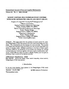
3.3. Fuzzy Logic System. A fuzzy logic system contains four parts [24], which are the knowledge base, the fuzzifier, the fuzzy inference engine working on fuzzy rules, and the defuzzifier, respectively. The primal fuzzy system is fixed and uniformity. To hold the consistent performance of the fuzzy system under this circumstance where there is a lot of uncertainty or unknown development tendency in system parameters and structures, the fuzzy system should possess adaptive performance. Without loss of generality, the output of an uncertain system can be assumed as 𝑓(𝜔). The fuzzy inference engine adopts the fuzzy if-then rules to form a mapping from an input vector 𝜔 = [𝜔1 , . . . , 𝜔𝑛 ]𝑇 ∈ 𝑅𝑛 to an output variable 𝑦 ∈ 𝑅. The 𝑖th fuzzy rule is of the form 𝑅𝑖 : If 𝜔1 is 𝜇1𝑖 and . . . 𝜔𝑛 is 𝜇𝑛𝑖 , then 𝑦 is 𝐵𝑖 , where 𝜇1𝑖 , . . . , 𝜇𝑛𝑖 and 𝐵𝑖 are fuzzy sets characterized by fuzzy membership functions, for example, the Gaussian type. Take the singleton fuzzifier, the product inference engine, and the center-average defuzzifier; then, the output variable 𝑦 can be described as 𝑦=

̃𝑖 ∏𝑛𝑗=1 𝜇𝑗𝑖 (𝜔𝑗 ) ∑𝑁 𝑖=1 𝑦 𝑛 𝑖 ∑𝑁 𝑖=1 (∏𝑗=1 𝜇𝑗 (𝜔𝑗 ))

= 𝜃T 𝜓 (𝜔) ,

(16)

where 𝑁 is the number of fuzzy rules, 𝜃 = [𝑦̃1 , . . . , 𝑦̃𝑁]T with 𝑦̃𝑖 being an adjustable value where the fuzzy membership function 𝜇𝐵𝑖 (𝑦̃𝑖 ) has the maximum value, choosing 𝜇𝐵𝑖 (𝑦̃𝑖 ) = 1 usually, and 𝜓(𝜔) = [𝜓1 , . . . , 𝜓𝑁]T is a fuzzy basis vector, whose element is of the form 𝜓𝑙 =

∏𝑛𝑗=1 𝜇𝑗𝑖 (𝜔𝑗 ) 𝑛 𝑖 ∑𝑁 𝑖=1 (∏𝑗=1 𝜇𝑗 (𝜔𝑗 ))

, 𝑙 = 1, . . . , 𝑁.

(17)

And the adaptive fuzzy system can be considered as the type of a neural network, which is shown in Figure 1 [24–26]. 3.4. Fuzzy Approximators. In this subsection we propose the use of fuzzy system to estimate the unknown function ̈ Then, the approximation is sued to develop a well𝑓(𝑞, 𝑞,̇ 𝑞). defined adaptive controller with its adaptation law in order to satisfy control objective.

4

Mathematical Problems in Engineering

First, for reducing the number of fuzzy rules hereinbelow, the uncertainty 𝑓(𝑞, 𝑞,̇ 𝑞)̈ can be represented as an addition of two functions: 𝑓 (𝑞, 𝑞,̇ 𝑞)̈ = 𝑓1 (𝑞, 𝑞)̇ + 𝑓2 (𝑞, 𝑞)̈ ,

T

𝑑11 ⋅ ⋅ ⋅ 𝑑1𝑛 [ ] [ .. ] 𝐷 = [ . d ... ] . [ ] ⋅ ⋅ ⋅ 𝑑 𝑑 𝑛𝑛 ] [ 𝑛1

(18)

where (19)

𝑓2 (𝑞, 𝑞)̈ = −𝑀0−1 (𝑞) Δ𝑀 (𝑞) 𝑞.̈

𝑓 (𝑞, 𝑞 ̇ | 𝜃 ) =

[𝜃11T 𝐹1

(𝑞, 𝑞)̇ , . . . , 𝜃𝑛1T 𝐹1

̇ (𝑞, 𝑞)]

𝑛

𝑛

𝑗−𝑛 𝑛

𝑖=1

𝑖=1

𝑗=1 𝑖=1

𝑎T 𝐷𝑐 = [∑𝑎𝑖 𝑑𝑖1 ⋅ ⋅ ⋅ ∑𝑎𝑖 𝑑𝑖1𝑛 ] 𝑐 = ∑ ∑𝑎𝑖 𝑑𝑖𝑗 𝑐𝑗 .

And each function will be replaced by the fuzzy logic system 𝑓̂1 (𝑞, 𝑞 ̇ | 𝜃1 ) and 𝑓̂2 (𝑞, 𝑞 ̈ | 𝜃2 ), respectively, which are of the form of (16) and (17): 1

𝑎1 𝑐1 ⋅ ⋅ ⋅ 𝑎1 𝑐𝑛 [ ] [ ] 𝑎𝑐T = [ ... d ... ] . [ ] 𝑎 𝑐 ⋅ ⋅ ⋅ 𝑎 𝑐 𝑛 𝑛] [ 𝑛1

T

T ̈ 𝑓̂2 (𝑞, 𝑞 ̈ | 𝜃2 ) = [𝜃12T 𝐹2 (𝑞, 𝑞)̈ , . . . , 𝜃𝑛2T 𝐹2 (𝑞, 𝑞)]

(20)

𝑑11 ⋅ ⋅ ⋅ 𝑑𝑛1 𝑎1 𝑐1 ⋅ ⋅ ⋅ 𝑎1 𝑐𝑛 [ ][ ] [ .. ] [ ] . 𝐷 𝑎𝑐 = [ . d .. ] [ ... d ... ] [ ][ ] 𝑑 𝑎 ⋅ ⋅ ⋅ 𝑑 𝑐 ⋅ ⋅ ⋅ 𝑎 𝑐 𝑛𝑛 ] [ 𝑛 1 𝑛 𝑛] [ 1𝑛 T

Thus, there is

𝑛

𝑛

[∑𝑑𝑖1 𝑎𝑖 𝑐1 ⋅ ⋅ ⋅ ∑𝑑𝑖1 𝑎𝑖 𝑐𝑛 ] [ 𝑖=1 ] 𝑖=1 [ ] .. .. [ ] =[ ], . d . [ ] [𝑛 ] 𝑛 [ ] ∑𝑑𝑖𝑛 𝑎𝑖 𝑐1 ⋅ ⋅ ⋅ ∑𝑑𝑖𝑛 𝑎𝑖 𝑐𝑛 [𝑖=1 ] 𝑖=1

𝜀1 = 𝑓1 (𝑞, 𝑞)̇ − 𝜃1∗T 𝐹1 (𝑞, 𝑞)̇ (22)

(29)

so

And they are bounded according to the approximation principle of the fuzzy logic; that is to say, there are very small positive constants 𝜎1 and 𝜎2 satisfying

𝑗=𝑛 𝑛

tr (𝐷T 𝑎𝑐T ) = ∑ ∑𝑎𝑖 𝑑𝑖𝑗 𝑐𝑗

(30)

𝑗=1 𝑖=1

is equal to the left.

󵄨 󵄨 𝜎1 ≥ 󵄨󵄨󵄨󵄨𝜀𝑖1 󵄨󵄨󵄨󵄨 , 󵄨 󵄨 𝜎2 ≥ 󵄨󵄨󵄨󵄨𝜀𝑖2 󵄨󵄨󵄨󵄨 ,

(23)

where 𝜀𝑖1 and 𝜀𝑖2 denote the 𝑖th element of the vector 𝜀1 and 𝜀2 . Define the approximation error of weight matrices as 𝜃̃1 = 𝜃1 − 𝜃1∗ , (24)

𝜃̃2 = 𝜃2 − 𝜃2∗ . 3.5. Two Lemmas

Lemma 3. If 𝑎, 𝑐 ∈ 𝑅𝑛 are row vectors, 𝐷 ∈ 𝑅𝑛×𝑛 is a square matrix; then there is T

T

(21)

Letting the optimal parameter matrices of the fuzzy logic system be 𝜃1∗ and 𝜃2∗ , respectively, the minimum approximation error vectors can be defined as follows:

T

(28)

Then

= 𝜃2T 𝐹2 (𝑞, 𝑞)̈ .

𝜀2 = 𝑓2 (𝑞, 𝑞)̈ − 𝜃2∗T 𝐹2 (𝑞, 𝑞)̈ .

(27)

On the right, first

= 𝜃1T 𝐹1 (𝑞, 𝑞)̇

𝑓̂ (𝑞, 𝑞,̇ 𝑞)̈ = 𝜃1T 𝐹1 (𝑞, 𝑞)̇ + 𝜃2T 𝐹2 (𝑞, 𝑞)̈ .

(26)

On the left,

𝑓1 (𝑞, 𝑞)̇ = −𝑀0−1 (𝑞) Δℎ (𝑞, 𝑞)̇ ,

̂1

T

Proof. Let a = [𝑎1 ⋅ ⋅ ⋅ 𝑎𝑛 ] , 𝑐 = [𝑐1 ⋅ ⋅ ⋅ 𝑐𝑛 ] , and

T

𝑎 𝐷𝑐 = tr (𝐷 𝑎𝑐 ) .

(25)

According to Barbalat’s lemma [22], If one function 𝑓(𝑡) is uniformly continuous on [0, +∞) and its general integral exists, then lim𝑡→∞ 𝑓(𝑡) = 0. 3.6. Main Result. In order to eliminate the effects of the approximation error and the external disturbance, we design the second part 𝑢𝑠𝑙 in (15) as follows: 𝑢𝑠𝑙 = −𝑘𝑠𝑙 sgn (𝛿) ,

(31)

where 𝛿 = [𝑃21 𝑃22 ] 𝑆 is the defined filtered error. 𝑃21 and 𝑃22 come from the solution 𝑃 of the Lyapunov equation (12), and the positive definite solution 𝑃 has the following form: 𝑃11 𝑃21 ]. 𝑃=[ 𝑃21 𝑃22

(32)

Mathematical Problems in Engineering

5

2

Fuzzy logic system

qd̈

q̈ Update laws 2̇

d/dt



e ̇

e

1



qḋ

d/dt

Fuzzy logic system

Update laws 1̇

d/dt

e

qd

d/dt

ual

ksl

P ė

 

ksl ＭＡＨ()

q̇

M(q) u

usl

d/dt Robot

M(q)u + ℎ(q, q)̇



manip-

q

ulator ℎ(q, q)̇

Figure 2: Architecture of the control scheme.

And 𝑘𝑠𝑙 is the control gain given by the following expression: 1

2

𝑘𝑠𝑙 = (𝜎 + 𝜎 + 𝑑0 ) 𝐼𝑛 ,

(33)

𝑛

where sgn(𝛿) ∈ 𝑅 is a switching function vector, whose common element is a switching function in scalar case: 1 𝛿𝑖 > 0 { { { { sgn𝑖 (𝛿𝑖 ) = {0 𝛿𝑖 = 0 { { { {−1 𝛿𝑖 < 0,

(34)

where 𝛿𝑖 ∈ 𝛿 (𝑖 = 1, 2, . . . , 𝑛). The block diagram of the control scheme is shown in Figure 2. Substituting (13), (15), (21)∼(22), (31), and (33) into (6), we obtain the following error dynamics: 𝑆 ̇ = 𝐴𝑆 + 𝐵, where 𝐵 = [0

T

(35)

T T

𝑏 ] and

𝑏 = −𝜃̃1T 𝐹1 (𝑞, 𝑞)̇ − 𝜃̃2T 𝐹2 (𝑞, 𝑞)̈ + 𝜀1 + 𝜀2 + 𝑢𝑠𝑙 + 𝑑.

(36)

The weight matrix updating algorithms are chosen as follows: 𝜃1̇ = 𝜂1 𝐹1 (𝑞, 𝑞)̇ 𝛿T , (37) 𝜃2̇ = 𝜂2 𝐹2 (𝑞, 𝑞)̈ 𝛿T ,

where 𝜂1 and 𝜂2 are positive constants. Considering (24), there are always ̇1 𝜃̃ = 𝜃1̇ ,

(38)

̇2 𝜃̃ = 𝜃2̇ .

Theorem 4. Considering more concise expression (6) of system (1), if the controller is synthesized by (13), (15), (31), and (33) and the weight matrix is adjusted by adaptive mechanism (37), then the trajectory tracking error of system (6) converges to zero asymptotically. Proof. Construct a Lyapunov function as follows: 1 1 𝑉 = 𝑆T 𝑃𝑆 + tr (𝜃̃1T 𝜂1−1 𝜃̃1 ) + 2 2 where 𝑃 is a solution of (12). Differentiate 𝑉 with respect to (35), under (32) and (36), yielding

1 ̃2T −1 ̃2 tr (𝜃 𝜂2 𝜃 ) , 2

(39)

the state trajectories of

1 1 1 𝑉̇ = 𝑆T (𝑃𝐴 + 𝐴T 𝑃) 𝑆 + 𝐵T 𝑃𝑆 + 𝑆T 𝑃𝐵 2 2 2 ̇1 ̇2 + tr (𝜃̃1T 𝜂1−1 𝜃̃ ) + tr (𝜃̃2T 𝜂2−1 𝜃̃ ) 0 1 1 1 = − 𝑆T 𝑄𝑆 + [0T 𝑏T ] 𝑃𝑆 + 𝑆T 𝑃 [ ] 2 2 2 𝑏

6

Mathematical Problems in Engineering

m2 l2

q2

m1 l1 q1

Figure 3: Two-link robotic manipulator.

̇1 ̇2 + tr (𝜃̃1T 𝜂1−1 𝜃̃ ) + tr (𝜃̃2T 𝜂2−1 𝜃̃ )

In fact, take (23) and Remark 2 into consideration; when 𝛿𝑖 ≥ 0, the latter part of (42) satisfies

𝑃21 1 1 1 = − 𝑆T 𝑄𝑆 + 𝑏T [𝑃21 𝑃22 ] 𝑆 + 𝑆T [ ] 𝑏 2 2 2 𝑃22

(𝜀𝑖1 + 𝜀𝑖2 − (𝜎1 + 𝜎2 + 𝑑0 ) sgn (𝛿𝑖 ) + 𝑑𝑖 ) 𝛿𝑖 = (𝜀𝑖1 + 𝜀𝑖2 − (𝜎1 + 𝜎2 + 𝑑0 ) + 𝑑𝑖 ) 𝛿𝑖 ≤ 0.

̇1 ̇2 + tr (𝜃̃1T 𝜂1−1 𝜃̃ ) + tr (𝜃̃2T 𝜂2−1 𝜃̃ )

And when 𝛿𝑖 < 0, the latter part of (42) satisfies (𝜀𝑖1 + 𝜀𝑖2 − (𝜎1 + 𝜎2 + 𝑑0 ) sgn (𝛿𝑖 ) + 𝑑𝑖 ) 𝛿𝑖

1 ̇1 = − 𝑆T 𝑄𝑆 + 𝑏T 𝛿 + tr (𝜃̃1T 𝜂1−1 𝜃̃ ) 2

= (𝜀𝑖1 + 𝜀𝑖2 + (𝜎1 + 𝜎2 + 𝑑0 ) + 𝑑𝑖 ) 𝛿𝑖 ≤ 0.

2

̇ + tr (𝜃̃2T 𝜂2−1 𝜃̃ ) 1 = − 𝑆T 𝑄𝑆 − 𝐹1T (𝑞, 𝑞)̇ 𝜃̃1 𝛿 − 𝐹2T (𝑞, 𝑞)̈ 𝜃̃2 𝛿 2 T ̇1 + (𝜀1 + 𝜀2 + 𝑢𝑠𝑙 + 𝑑) 𝛿 + tr (𝜃̃1T 𝜂1−1 𝜃̃ ) 2

̇ + tr (𝜃̃2T 𝜂2−1 𝜃̃ ) . (40) Further, substitute the adaptive updating rules (37) and (38) into the above expression, and use Lemma 3, obtaining T 1 𝑉̇ = − 𝑆T 𝑄𝑆 + (𝜀1 + 𝜀2 + 𝑢𝑠𝑙 + 𝑑) 𝛿. 2

(41)

Then, substitute (31) and (33) into 𝑉,̇ displaying 1 𝑉̇ = − 𝑆T 𝑄𝑆 2 1

2

1

2

T

(42)

+ (𝜀 + 𝜀 − (𝜎 + 𝜎 + 𝑑0 ) sgn (𝛿) + 𝑑) 𝛿. Considering (34), no matter 𝛿𝑖 > 0, 𝛿𝑖 = 0 or 𝛿𝑖 < 0, there are always 1 𝑉̇ ≤ − 𝑆T 𝑄𝑆 ≤ 0. 2

(44)

(43)

(45)

Now, we have proved that the Lyapunov function 𝑉 decreases monotonically. Thus, it can be concluded that the close loop system is globally stable and 𝑆, 𝜃̃1 , 𝜃̃2 are uniformly bounded. Furthermore, it is easy to show that 𝜃1 and 𝜃2 are unï we can formly bounded too. With boundedness of 𝑓(𝑞, 𝑞,̇ 𝑞), 1 1 2 2 ̂ ̂ say that the estimations 𝑓 (𝑞, 𝑞 ̇ | 𝜃 ) and 𝑓 (𝑞, 𝑞 ̈ | 𝜃 ) are also bounded. Thus, it can be concluded that 𝑢𝑎𝑙 in (13) and 𝑢𝑠𝑙 in (31) are uniformly bounded. That is to say, all the right parts of (36) are bounded, and hence 𝑏 is bounded. Therefore, (35) implies that 𝑆 ̇ is uniformly bounded, which tells us that 𝑆 will be uniformly continuous. 𝑡 Let 𝑉1 = 𝑉 − ∫0 (𝑉̇ + (1/2)𝑆T 𝑄𝑆)𝑑𝜏. Because of the existence of 𝑉̇ ≤ −1/2𝑆T 𝑄𝑆, then 𝑉1 (𝑡) ≥ 0, so we can say that 𝑉1 (𝑡) has below boundedness. Further, as 𝑉1̇ = −1/2𝑆T 𝑄𝑆, then 𝑉1̇ ≤ 0; that is, 𝑉1̇ is semi-negativedefinite. Finally, the uniform continuousness of 𝑆 will make 𝑉1̇ uniformly continuous too. Hence, using Barbalat’s lemma, we can deduce that lim 𝑉1 = 0; that is, when 𝑡 → ∞, we have 𝑆 → 0. Then the tracking error 𝑒 and its derivative 𝑒 ̇ converge to zero asymptotically.

4. Simulations Results In this section, we will take a two-link manipulator to verify the feasibility of the suggested controller. The configuration of the manipulator and its parameters are shown in Figure 3 [27–29].

Mathematical Problems in Engineering

7

The symbols in (1) are described as follows: 𝑀 (𝑞) = [

𝑀11 𝑀12 𝑀21 𝑀22

], (46)

ℎ1

ℎ (𝑞, 𝑞)̇ = [ ] , ℎ2 where ℎ1 = −𝑚2 𝑙1 𝑙2 sin(𝑞2 )𝑞2̇ (𝑞1̇ + 𝑞2̇ ) + (𝑚1 + 𝑚2 ) cos(𝑞2 )𝑔, ℎ2 = 𝑚2 𝑙1 𝑙2 sin(𝑞2 )𝑞12̇ , 𝑀11 = (𝑚1 + 𝑚2 )𝑙12 , 𝑀22 = 𝑚2 𝑙22 , and 𝑀12 = 𝑀21 = 𝑚2 𝑙1 𝑙2 cos(𝑞1 − 𝑞2 ). The values of these body parameters are simply chosen as 𝑚1 = 𝑚2 = 1 (kg) and 𝑙1 = 𝑙2 = 1 (m). The initial angles are chosen as 𝑞1 (0) = 𝑞2 (0) = 0, and their derivatives are 𝑞1̇ (0) = 𝑞2̇ (0) = 0. The desired reference trajectories are selected as 𝑞𝑑1 = sin 𝑡 and 𝑞𝑑2 = 2 sin 𝑡. Let the outside disturbance T be 𝜏𝑑 = [0.5 cos(𝑡) 0.5 sin(𝑡)] . Other parameters are 𝛼 = 1 2 𝛽 = 100𝐼2 , 𝜎 = 𝜎 = 1, 𝜂 = 0.1, 𝑑0 = 0.5, and 𝑄 = 𝐼4 . In simulations, we choose five fuzzy levels, that is, NB, NS, ZO, PS, and PB on the universe of each input variable and we use the following Gaussian membership function [24]: 2

𝑥 − 𝑥𝑙𝑖 ] ) , 𝜇𝐴𝑙𝑖 (𝑥𝑖 ) = exp [− ( 𝑖 𝜋/24 [ ]

(47)

where 𝑥𝑙𝑖 are −𝜋/6, −𝜋/12, 0, 𝜋/12, and 𝜋/6, respectively. When the modeling uncertainties Δ𝑀(𝑞) and Δℎ(𝑞, 𝑞)̇ change by 20%, the corresponding simulation results are shown in Figures 4(a) and 4(b). From these simulation results, we can see that the designed controller guarantees actual trajectory tracking of the desired one completely. Meanwhile, when the uncertainties Δ𝑀(𝑞) and Δℎ(𝑞, 𝑞)̇ change in a greater range, for example 50%, the corresponding simulation results are listed in Figures 4(c) and 4(d). Figure 4(c) tells us that in this case there are tracking trajectory errors. However, if we make parameters 𝛼 and 𝛽 larger, for example, let 𝛼 = 𝛽 = 500𝐼2 , then there are no tracking trajectory errors again. This is shown in Figures 4(e) and 4(f), while Figure 4(f) indicates that when these uncertainties change in a bigger width and parameters 𝛼, 𝛽 are larger, the control inputs tend to be more bad. In order to investigate the performance of the proposed controllers, we will give a simulated comparison of the robust control scheme [23, 30] in the end of this chapter. In this ̇ ̈ −𝛼𝑒−𝛽𝑒) ̇ scheme, (4) becomes 𝜏 = ℎ0 (𝑞, 𝑞)+𝑀 0 (𝑞)𝑢+𝑀0 (𝑞𝑑 and the controller 𝑢 = −𝐵T 𝑃𝑆𝜌2 /(|𝑆T 𝐵𝑃|𝜌 + 𝛾), where 𝐵 is selected as 𝐵 = [0, 0; 0, 0; 1, 0; 0, 1], that is, the same as [23, 30], 𝑃 is a solution of the Lyapunov equation (12), 𝛾 is a very small positive number chosen as 𝛾 = 0.001, and 𝜌 describes the upper bound of modeling uncertainties Δ𝑀(𝑞) ̇ which can be chosen with a greater value than and Δℎ(𝑞, 𝑞), the upper bound of the modeling uncertainties, such as 𝜌 = 10. All of the other used expressions and parameters do not change.

The simulation results adopting robust control scheme are shown in Figure 5, where Figures 5(a) and 5(b) are obtained when the modeling uncertainties Δ𝑀(𝑞) and Δℎ(𝑞, 𝑞)̇ change by 20%, Figures 5(c) and 5(d) are obtained when the modeling uncertainties Δ𝑀(𝑞) and Δℎ(𝑞, 𝑞)̇ change by 50%, and Figures 5(e) and 5(f) are also obtained when the modeling uncertainties change by 50%, but in the case of 𝛼 = 𝛽 = 200𝐼2 rather than 𝛼 = 𝛽 = 100𝐼2 which are used in Figures 5(a), 5(b), 5(c), and 5(d). From these simulations results, we can see that the proposed controller in this paper is very effective and shows higher precision. In fact, [23, 30] tell us that the robust controller 𝑢 = −𝐵T 𝑃𝑆𝜌2 /(|𝑆T 𝐵𝑃|𝜌 + 𝛾) can only guarantee global uniform ultimate boundedness rather than global asymptotic stability.

5. Conclusion This paper proposes an adaptive fuzzy control scheme for uncertain robotic system. Although the control scheme is proposed for uncertain robotic system, it can be suitable for a kind of MIMO system. First, we prove our control scheme effectiveness based on Lyapunov method. Then, we take a two-link manipulator to verify the feasibility of the suggested controller. The simulation results tells us that what we do is very meaningful. However, it should be noted that the variable structure term sgn(𝛿) is adopted to increase the robust performance, but it will generate “chattering” phenomenon, which may irritate unmolded high-frequency dynamics and even destroy the physical device. In order to weaken or eliminate the “chattering,” there are some good directions stated as follows. (1) The saturation function method, which is described below, can be used when frequency is too high, but using the saturation may degrade the robustness. It is very important to choose an appropriate boundary layer thickness 𝜇. 𝛿 { { {sgn ( 𝜇 ) , sat (𝛿) = { { {𝛿 {𝜇

󵄨󵄨 𝛿 󵄨󵄨 󵄨󵄨 󵄨󵄨 󵄨󵄨 󵄨󵄨 ≥ 1 󵄨󵄨 𝜇 󵄨󵄨 󵄨󵄨 𝛿 󵄨󵄨 󵄨󵄨 󵄨󵄨 󵄨󵄨 󵄨󵄨 < 1. 󵄨󵄨 𝜇 󵄨󵄨

(48)

(2) Adjust the term gain switching online, study a new sliding mode control method, and so on.

Conflicts of Interest The authors declare that they have no conflicts of interest.

Acknowledgments This work is supported by the National Natural Science Foundation of China (11371221), the Natural Science Foundation of Shandong Province of China (ZR2014AM032), and the Project of Shandong Province Higher Educational Science and Technology Program (J16LI15).

Mathematical Problems in Engineering

0 −1 −2

0

1

2

3

4 5 6 time (s)

7

8

9 10

Control input 1

1 600 400 200 0 −200

Control input 2

Position tracking 1

8

400

Position tracking 2

qd1 q1 4 2 0 −2

0

1

2

3

4 5 6 time (s)

7

8

9 10

0

1

2

3

4 5 6 time (s)

7

8

9 10

0

1

2

3

4 5 6 time (s)

7

8

9 10

200 0 −200

qd2 q2 Position tracking 1

(a) Tracking trajectory

(b) Control input

1

0

1

2

3

4 5 6 time (s)

7

8

9 10

Control input 1

−2

600 400 200 0 −200

Control input 2

0 −1

400

Position tracking 2

qd1 q1 4 2 0 −2

0

1

2

3

4 5 6 time (s)

7

8

9 10

0

1

2

3

4 5 6 time (s)

7

8

9 10

0

1

2

3

4 5 6 time (s)

7

8

9 10

200 0 −200

qd2 q2 (d) Control input

0

1

2

3

4 5 6 time (s)

7

8

9 10

Control input 1

Position tracking 1

(c) Tracking trajectory

1 0.5 0 −0.5 −1 −1.5

600 400 200 0 −200

3 2 1 0 −1 −2

Control input 2

Position tracking 2

qd1 q1

0

1

2

3

4 5 6 time (s)

7

8

9 10

400 300 200 100 0 −100

0

1

2

3

4 5 6 time (s)

7

8

9 10

0

1

2

3

4 5 6 time (s)

7

8

9 10

qd2 q2 (e) Tracking trajectory

(f) Control input

Figure 4: Simulation results with proposed controller.

9

1

−1 −2

0

1

2

3

4 5 6 time (s)

7

8

9 10

Control input 1

0 600 400 200 0 −200

Control input 2

Position tracking 1

Mathematical Problems in Engineering

400 300 200 100 0 −100

Position tracking 2

qd1 q1 3 2 1 0 −1 −2

0

1

2

3

4 5 6 time (s)

7

8

9 10

0

1

2

3

4 5 6 time (s)

7

8

9 10

0

1

2

3

4 5 6 time (s)

7

8

9 10

qd2 q2 (b) Control input

−2

0

1

2

3

4 5 6 time (s)

7

8

9 10

Control input 1

0 −1

600 400 200 0 −200

Control input 2

Position tracking 1

(a) Tracking trajectory

1

400 300 200 100 0 −100

Position tracking 2

qd1 q1 3 2 1 0 −1 −2

0

1

2

3

4 5 6 time (s)

7

8

9 10

0

1

2

3

4 5 6 time (s)

7

8

9 10

0

1

2

3

4 5 6 time (s)

7

8

9 10

qd2 q2 (d) Control input

−1 −2

0

1

2

3

4 5 6 time (s)

7

8

9 10

Control input 1

0 600 400 200 0 −200

Control input 2

Position tracking 1

(c) Tracking trajectory

1

400 300 200 100 0 −100

Position tracking 2

qd1 q1 3 2 1 0 −1 −2

0

1

2

3

4 5 6 time (s)

7

8

9 10

0

1

2

3

4 5 6 time (s)

7

8

9 10

0

1

2

3

4 5 6 time (s)

7

8

9 10

qd2 q2 (e) Tracking trajectory

(f) Control input

Figure 5: Simulation results with robust controller.

10

References [1] L. Wang, T. Chai, and C. Yang, “Neural-network-based contouring control for robotic manipulators in operational space,” IEEE Transactions on Control Systems Technology, vol. 20, no. 4, pp. 1073–1080, 2012. [2] L. Yu, S. Fei, J. Huang, and Y. Gao, “Trajectory switching control of robotic manipulators based on RBF neural networks,” Circuits, Systems and Signal Processing, vol. 33, no. 4, pp. 1119– 1133, 2014. [3] M. Kemmotsu and Y. Mutoh, “Control system of robot manipulator using linear time-varying controller design technique,” in Proceedings of the 33rd Chinese Control Conference, pp. 28–30, Nanjing, China, 2014. [4] T. Mai, Y. Wang, and T. Ngo, “Adaptive tracking control for robot manipulators using fuzzy wavelet neural networks,” International Journal of Robotics and Automation, vol. 30, no. 1, pp. 26–39, 2015. [5] K. Kherraz, M. Hamerlain, and N. Achour, “Robust neurofuzzy sliding mode controller for a flexible robot manipulator,” International Journal of Robotics and Automation, vol. 30, no. 1, pp. 40–49, 2015. [6] C. W. Tao, J. S. Taur, and M.-L. Chan, “Adaptive fuzzy terminal sliding mode controller for linear systems with mismatched time-varying uncertainties,” IEEE Transactions on Systems, Man, and Cybernetics, Part B: Cybernetics, vol. 34, no. 1, pp. 255– 262, 2004. [7] M. Chen, Q. Wu, C. Jiang, and B. Jiang, “Guaranteed transient performance based control with input saturation for near space vehicles,” Science China Information Sciences, vol. 57, no. 5, pp. 1–12, 2014. [8] A. Boulkroune, M. Tadjine, M. M’Saad, and M. Farza, “How to design a fuzzy adaptive controller based on observers for uncertain affine nonlinear systems,” Fuzzy Sets and Systems, vol. 159, no. 8, pp. 926–948, 2008. [9] V. Nekoukar and A. Erfanian, “Adaptive fuzzy terminal sliding mode control for a class of MIMO uncertain nonlinear systems,” Fuzzy Sets and Systems, vol. 179, no. 1, pp. 34–49, 2011. [10] Z. B. Du and S. S. Hu, “Fuzzy mixed H2 /H∞ sampled-data control for nonlinear systems,” Control and Decision, vol. 32, no. 5, pp. 930–934, 2017. [11] R. H. Du, Y. F. Wu, W. Chen, and Q. W. Chen, “Adaptive backstepping fuzzy control for servo systems with backlash,” Control Theory & Applications, vol. 30, no. 2, pp. 254–260, 2013 (Chinese). [12] J. Fei and J. Zhou, “Robust adaptive control of MEMS triaxial gyroscope using fuzzy compensator,” IEEE Transactions on Systems, Man, and Cybernetics, Part B: Cybernetics, vol. 42, no. 6, pp. 1599–1607, 2012. [13] X. Bu, X. Wu, Z. Ma, and Y. Zhong, “Design of a modified arctangent-based tracking differentiator,” Journal of Shanghai Jiaotong University, vol. 49, no. 2, pp. 164–168, 2015. [14] C. Ham, Z. Qu, and R. Johnson, “Robust fuzzy control for robot manipulators,” IEE Proceedings Control Theory and Applications, vol. 147, no. 2, pp. 212–216, 2000. [15] Y. Q. Wei, J. D. Zhang, L. Hou, and Q. L. Chang, “Backstepping adaptive fuzzy control for two-link robot manipulators,” vol. 10, pp. 303–308, 2013. [16] M. M. Azimi and H. R. Koofigar, “Adaptive fuzzy backstepping controller design for uncertain underactuated robotic systems,” Nonlinear Dynamics, vol. 79, no. 2, pp. 1457–1468, 2014.

Mathematical Problems in Engineering [17] J. Fei and H. Ding, “Adaptive sliding mode control of dynamic system using RBF neural network,” Nonlinear Dynamics, vol. 70, no. 2, pp. 1563–1573, 2012. [18] J. Fei and C. Lu, “Adaptive sliding mode control of dynamic systems using double loop recurrent neural network structure,” IEEE Transactions on Neural Networks and Learning Systems, vol. 29, no. 4, pp. 1275–1286, 2017. [19] F. Lin, Robust Control Design: An Optimal Control Approach, John Wiley & Sons, Chichester, UK, 2007. [20] F. O. Rodriguez, J. J. Rubio, C. R. Gaspar, J. C. Tovar, and M. A. Armendariz, “Hierarchical fuzzy CMAC control for nonlinear systems,” Neural Computing and Applications, vol. 23, no. 1, pp. 323–331, 2013. [21] J. L. Zhou and W. H. Zhang, “Robust control for robots based on linear state equation,” in Proceedings of the 3rd International Conference on Impulsive Dynamical Systems and Applications, pp. 454–459, Qingdao, China, 2006. [22] Z. H. Man and M. Palaniswami, “Robust tracking control for rigid robotic manipulators,” IEEE Transactions on Automatic Control, vol. 39, no. 1, pp. 154–159, 1994. [23] J. L. Zhou and W. H. Zhang, “Robust tracking control for a kind of robot traces,” Control Engineering of China, vol. 14, no. 3, pp. 336–339, 2007. [24] B. K. Yoo and W. C. Ham, “Adaptive control of robot manipulator using fuzzy compensator,” IEEE Transactions on Fuzzy Systems, vol. 8, no. 2, pp. 186–199, 2000. [25] S. Islam and P. X. Liu, “Robust adaptive fuzzy output feedback control system for robot manipulators,” IEEE/ASME Transactions on Mechatronics, vol. 16, no. 2, pp. 288–296, 2011. [26] F. C. Sun, Z. Q. Sun, and G. Feng, “Design of adaptive sliding mode controller for robot manipulators,” in Proceedings of the 5th IEEE Conference on Fuzzy Systems, pp. 817–823, New Orleans, La, USA, 1996. [27] K.-K. D. Young, “Controller design for a manipulator using theory of variable structure systems,” IEEE Transactions on Systems, Man, and Cybernetics, vol. 8, no. 2, pp. 101–109, 1978. [28] P. V. Cuong and W. Y. Nan, “Adaptive trajectory tracking neural network control with robust compensator for robot manipulators,” Neural Computing and Applications, vol. 27, no. 2, pp. 525–536, 2016. [29] J. Zhou, “Adaptive fuzzy finite-time control for uncertain robotic manipulator,” International Journal of Robotics and Automation, vol. 32, no. 2, pp. 134–141, 2017. [30] Y. Dai, S. Shi, and N. Zheng, “Class of robust control strategies for robot manipulators with uncertainties,” Acta Automatica Sinica, vol. 25, no. 2, pp. 204–209, 1999.

Advances in

Operations Research Hindawi www.hindawi.com

Volume 2018

Advances in

Decision Sciences Hindawi www.hindawi.com

Volume 2018

Journal of

Applied Mathematics Hindawi www.hindawi.com

Volume 2018

The Scientific World Journal Hindawi Publishing Corporation http://www.hindawi.com www.hindawi.com

Volume 2018 2013

Journal of

Probability and Statistics Hindawi www.hindawi.com

Volume 2018

International Journal of Mathematics and Mathematical Sciences

Journal of

Optimization Hindawi www.hindawi.com

Hindawi www.hindawi.com

Volume 2018

Volume 2018

Submit your manuscripts at www.hindawi.com International Journal of

Engineering Mathematics Hindawi www.hindawi.com

International Journal of

Analysis

Journal of

Complex Analysis Hindawi www.hindawi.com

Volume 2018

International Journal of

Stochastic Analysis Hindawi www.hindawi.com

Hindawi www.hindawi.com

Volume 2018

Volume 2018

Advances in

Numerical Analysis Hindawi www.hindawi.com

Volume 2018

Journal of

Hindawi www.hindawi.com

Volume 2018

Journal of

Mathematics Hindawi www.hindawi.com

Mathematical Problems in Engineering

Function Spaces Volume 2018

Hindawi www.hindawi.com

Volume 2018

International Journal of

Differential Equations Hindawi www.hindawi.com

Volume 2018

Abstract and Applied Analysis Hindawi www.hindawi.com

Volume 2018

Discrete Dynamics in Nature and Society Hindawi www.hindawi.com

Volume 2018

Advances in

Mathematical Physics Volume 2018

Hindawi www.hindawi.com

Volume 2018