creation, a new adaptive grid map building algorithm based on multiway tree is proposed. The environment ... autonomous map building in the field of robotics research ..... H.P. Moravec, A. Elfes, High resolution maps from wide-angle sonar.
MATEC Web of Conferences 160, 06001 (2018) https://doi.org/10.1051/matecconf/201816006001 EECR 2018
Adaptive GridMap Building Algorithm for Mobile Robot Based on Multiway Tree Jing Zhou
1,2
1,2
, Xiaogang Ruan , Pengfei Dong
1,2
and Jingjing Zhang
1,2
1
Faculty of Information Technology, Beijing University of Technology, Beijing 100124 , China Beijing Key Laboratory of Computational Intelligence and Intelligent System, Beijing 100124, China
2
Abstract.In order to solve the problem that uniform grid map occupies large storage space in the process of large-scale map creation, a new adaptive grid map building algorithm based on multiway tree is proposed. The environment map is divided into nine grids. The algorithm determines whether the grid is completely occupied, partially occupied or vacant. Then the part occupied gridsare further subdivided into smaller grids. The algorithm continues to determine whether the smaller grid is completely occupied, partially occupied or vacant.Repeat the above segmentation process until the entire map search is completed and the accuracy requirements are met. Finally, the scale of grid map does not depend on human experience but presenting adaptive characteristics. The algorithm is compared with the uniform grid method.The simulation results show that the algorithm has convergence.Andcompared with the uniform scale raster map, itgreatly saves the storage space.
1 Introduction Three key issues of mobile robot navigation are positioning, map building and path planning[1]. The autonomous map building in the field of robotics research is a fundamental and important problem, which is the precondition to achieve autonomous navigation. At present, the most widely used methods of map creation are geometric feature method, topological method and grid method. A geometric feature map is represented by related geometric features (points, lines, planes). This method can find the shortest path, but the disadvantage is that the more obstacles.The longer the search time, especially for the search of circular obstacles may be invalid. In 2011, Zhu Jianguo et al. [2] extracted linear features from lidar data to describe the environment. The established environmental feature maps were accurate and effective, and the data were small compared with raster maps. In 2013, GuoYupeng [3] used lidar data to extract the geometric features of the environment for the semantic classification of indoor environment. Topological map is a topological structure graph showing indoor environment as node and related connection line. The composition is fast and simple, but it is difficult to create large scale maps, and has no discrimination ability for similar or symmetrical scenes. In 1994, Gaussier P, ZrehenS[4] and other online learning topological graph were used to realize obstacle avoidance of mobile robot. In 2012, W Yan and others [5] built Growing Neural Gas (GNG) indoor environment cognitive map, and the robot's position was obtained through the global image machine on the ceiling. Wang
Dongshu et al. [6] constructed a model of nodes with growing neural gas network as a topological node, which makes the robot easy to understand the environment. In 2013, RuanXiaogang et al.[7] proposed a dynamically increasing and decreasing self-organizing feature map (DGPSOM) algorithm, which uses a small number of neurons to represent a large amount of environmental information. In 2017, Alitappeh, RJ, et al. [8] proposed an efficient distributed deployment strategy, which can optimize the allocation of robot teams in the environment of topological graph representation. Grid method is suitable for a variety of complex environments, and it is better than geometric feature method and topology method in modeling, updating and processing. Therefore, the method is favored by scholars and researchers in recent years. Grid map was first proposed by Elfes and Moraves[9] in 1985. The idea is to divide the whole work environment into homogeneous grids, and point out the possibility of obstacles in each grid. In 1990s, Konolige[10] and Thrun[11] established and optimized the grid map method, and applied it to the problems such as Simultaneous Localization and Mapping (SLAM). The geometric topological graph and the grid topological graph are established respectively for the sacred [12] and the ThrunS[13]. In 2010, Li Tiancheng[14] and so on based on fan grid map path planning for robots, increase the diversity of grid morphology. GuoLijin [15] and Duan Yong [16] section proposed the creation algorithm of adaptive grid map of variable precision, instead of the traditional uniform scale map with variable precision raster map. That saves the storage space. Although the grid method in robot environment cognition and map building showed many
© The Authors, published by EDP Sciences. This is an open access article distributed under the terms of the Creative Commons Attribution License 4.0 (http://creativecommons.org/licenses/by/4.0/).
MATEC Web of Conferences 160, 06001 (2018) https://doi.org/10.1051/matecconf/201816006001 MATEC Web of Conferences EECR 2018
The basic idea of adaptive raster map building algorithm stems from multiway tree. Different from the general multiway tree, this tree must follow two basic principles. (1)The gray node is uncertain state nodes. Each graynode should continue to be divided into nine sub nodes. (2)Black and white nodes determine the statement ofthenodes.Black represents to be completely occupied and white say vacant.They are leaf nodes, indivisible. The structure of the multiway tree is shown in Figure 1.
advantages, in the construction of large scale environment map.It still exists some shortcomings with the map to expand the scope and improves the grid resolution.The algorithm will consume huge storage space with great computational complexity. Therefore, in order to solve the problem of occupying large amount of memory space in the process of large scale map creation, a new adaptive raster map building algorithm based on multiway tree is proposed.
2 Related works 2.1 Method for creating uniform raster map The grid map usually refers to the traditional uniform scale raster map. The method first divides the external environment into many small units called grids. Then uses probability values to represent the possibility that each grid is occupied. A uniform scale raster map divides the whole environment into a homogeneous unit gridand each grid giving a value of 0-1 intervals to represent the state of the grid. 0 means completely empty, and 1 means full occupancy. In this way, the whole environment space can be divided into occupied space and vacant space. An environment map represented by a grid. The resolution of the environment space is related to the size of the grid. The traditional grid scale is determined by human experience.When the environment changes, you need to redetermine the scale by human experience. Increasing resolution means increasing computing time and computer memory consumption. With the expanding of human detection environment and unstructured environment, adding high dimensional entity, these not only lead to environmental information problem caused the massive increase of information storage, but fusion of massive data become more application of grid method for obstacle.
Figure 1. Multiway tree structure diagram.
3.2 Adaptive raster map creation process According to the principle of the multiway tree, an adaptive raster mapis created, which called variable precision raster map. The segmentation process of the raster map is shown in Figure 2. (1) The robot roughly circles around the whole environment, and divides the whole unknown environment into nine square structures. (2) Firstly, judge the nine sub grid state grid which is empty or occupied and which is in an unknown state. Secondly, the unknown grid environment for detailed exploration are further subdivided into small squares structure. (3) Update the map. (4) Repeat steps (2) and (3) until the entire map search is completed and the accuracy requirements are met. Then the composition is completed.
2.2 Grid method based on quadtree Document [9] adopts the principle of four fork tree to construct adaptive raster map, which belongs to a kind of variable precision raster map. The quadtree of each tree is divided into 4 sub nodes. Each node also has three states, according to the different state of continued segmentation. The composition will not stop until the entire map exists only completely occupied and vacant two states. The composition method optimizes the traditional method to a certain extent and saves the storage space, but the realtime composition of the composition needs to be improved. In this paper, the existing grid method is improved from two aspects of saving data storage space and improving the real-time composition.
3 Adaptive algorithm
raster
map
creation
3.1 The basic principle of multiway tree
Figure 2. Adaptive raster map creation process.
2
MATEC Web of Conferences 160, 06001 (2018) https://doi.org/10.1051/matecconf/201816006001 EECR 2018 EECR 2018
3.3 Adaptive raster map representation The father grid is in an unknown state grid segmentation, nine sub grid in the position number of the layer as shown in Figure 2. The N subdivision is obtained after the grid serial number is X 1 X 2 X 3 ... X n (n bits). X i , which according to the position of grid at the i layer, selecting from 0,1,2,3,4,5,6,7 and 8. For grids that continue to be down, taking the left to right order to add the location number of the sub grid to the back of the parent grid. If the grid number after three times splits is 152, a subdivision is continued.The nine sub grid is numbered1520, 1521, 1522, 1523, 1524, 1525, 1526, 1527, 1528. The location of the grid in the map can be obtained by grid numbers. The scale of the environment map is a b . The grid is numbered X 1 X 2 X 3 ... X n , and the central coordinate of the grid is (x, y).Then (x, y) can be expressed by the following formula.
Figure 3.Laser sensor ranging principle.
Estimate which grids are covered according to the position and pose of the robot X z ( s ) . Calculate the probability value of the covered grid and update it. The return value d (s ) and return value (s ) based sensor angle and distance are used to calculate the probability of obstacles in grid i. The algorithm is as follows.
1 1 1 1 1 x a ( 1 2 2 3 3 ... n n ) 2 3 3 3 3 1 1 1 1 1 y b ( 1 2 2 3 3 ... n n ) (1) 2 3 3 3 3
p{xi (s) OCC | X Z (s), d (s)}
(d i d min ) 2 (2) (d ( s) d min ) 2
p{xi ( s) OCC | X Z ( s), ( s)} 1
When X 1 , X 2 , X 3 ,..., X n take 0, 3, 6, 1 , 2 , 3 ,...., n =-1.
(i d min ) 2 (3)
max 2
Among them, d i is the distance between the robot
When X 1 , X 2 , X 3 ,..., X n take 1, 4, 7, 1 , 2 , 3 ,...., n =0.
and the center of the grid i. i is the angle between the x axis of the robot coordinate system and the center of the grid i. Assuming that the two events of d (s ) and
When X 1 , X 2 , X 3 ,..., X n take 2, 5, 8, 1 , 2 , 3 ,...., n =1.
(s) are independent of each other, the probability of obstacles in the grid i can be obtained according to the robot's current pose and sensor readings.
When X 1 , X 2 , X 3 ,..., X n take 0, 1, 2, 1 , 2 , 3 ,...., n =-1. When X 1 , X 2 , X 3 ,..., X n take 3, 4, 5, 1 , 2 , 3 ,...., n =0.
p{xi ( s) OCC | X Z ( s), D( s)}
p{xi ( s) OCC | X Z ( s), d ( s), ( s)}
When X 1 , X 2 , X 3 ,..., X n take 6, 7, 8, 1 , 2 , 3 ,...., n =1.
p{d ( s) | X Z ( s), ( s), xi ( s) OCC} p{xi ( s) OCC | X Z ( s), ( s)} /
p{d ( s) | X Z ( s), ( s)}
3.4Probability for occupying grids
(4)
p{d ( s) | X Z ( s), xi ( s) OCC}
Suppose the robot sensor detects the distance range [ d min , d max ] , the angle range is [min , max ] . The final
p{xi ( s) OCC | X Z ( s), ( s)} / p{d ( s) | X Z ( s)}
state of each gridis x i , namely one of two states, each
Also as we have
state {OCC , EMP} .Correspond to a probability value according to the probability value of the map update.The xi is set initial state probability of
p{d ( s ) | X Z ( s ), xi ( s ) OCC} p{xi ( s ) OCC | X Z ( s ), d ( s )} (5)
p{x i OCC} p{x i EMP} 0.5 , namely grid undetected. When the robot moves to steps, the sensor sees an obstacle in front of it and the sensor reads D (s ) = [d (s), (s)]T . As is shown in Figure 3.
p{d ( s ) | X Z ( s )} p{d ( s ) | X Z ( s )} p{xi ( s) OCC | X Z ( s)} p{d ( s ) | X Z ( s )} Therefore, the formula (4) is used
3
(6)
MATEC Web of Conferences 160, 06001 (2018) https://doi.org/10.1051/matecconf/201816006001 MATEC Web of Conferences EECR 2018
p{xi (s) EMP | X Z ( s), D( s)}
p{xi ( s ) OCC | X Z ( s ), D ( s )}
1 - p{xi ( s) OCC | X Z ( s), D( s)}
p{xi ( s ) OCC | X Z ( s ), d ( s )}
(7)
p{xi ( s ) OCC | X Z ( s ), ( s )} /
Next, you need to update the grid map. The convergence of the algorithm is proved that when the probability of the grid occupancy is greater than or equal to p max , the grid is occupied and represented by 1. However, when the probability of the occupancy of the grid is less than or equal to p min , the grid is considered empty and represented by 0. Besides, when the grid scale is less than half of the length and width of the robot, it is no longer subdivided. Under this condition, if the minimum level of the grid is occupied by a probability greater than 0. Otherwise, the grid is assumed to be occupied and represented by 1. If the smallest grid is occupied, the probability is equal to 0 and the grid is empty, expressed in 0. According to the above analysis, it can be seen that the environment map constructed by the algorithm has the condition of ending the segmentation explicitly. So the convergence of the adaptive grid algorithm is proved.
p{xi ( s ) OCC | X Z ( s )}
Similarly, according to the robot's current pose and sensor readings, the probability that there is no obstacle in the grid i can be obtained. p{xi ( s ) EMP | X Z ( s ), D( s )} p{xi ( s ) EMP | X Z ( s ), d ( s )}
(8)
p{xi ( s ) EMP | X Z ( s), ( s )} / p{xi ( s ) EMP | X Z ( s)}
Also as we have p{xi ( s) EMP | X Z (s), D( s)}
(9)
1 p{xi (s) OCC | X Z (s), D(s)} p{xi ( s) EMP | X Z ( s), d( s)} 1 p{xi ( s) OCC | X Z ( s), d( s)}
p{xi (s) EMP | X Z ( s), ( s)}
1 p{xi ( s) OCC | X Z (s), (s)}
(15)
(10)
4 Simulation experiment
(11)
Suppose that the simulation environment is a 50m 50m static indoor environment, as isshown in Figure 4.
And at the statement of without having the sensor observation value D (s) p{xi (s) EMP | X Z (s)} p{xi (s) OCC | X Z (s)}
(12)
Substitute (8) ~ (11) for (7) p{xi ( s ) OCC | X Z ( s)} 1 [1 p{xi ( s ) OCC | X Z ( s), d( s)}] [1 p{xi ( s) OCC | X Z ( s ), ( s)}] /
(13)
[1 p{xi ( s ) OCC | X Z ( s ), D( s )}] Figure 4.Static simulation environment.
To substitute (13) for (7)
The simulation experiment is carried out on the Turtlebot2 robot simulation system and the robot diameter is 42cm. The data collection of motion model is completed by odometer and gyroscope. The data acquisition of measurement model is completed by RPLIDAR-A2 360 degree laser radar scanner. The laser radar’s height is 40.5mm, and the width is 72.5mm. The range of distance is the best of 0.15m~8m. The scanning angle is from 0 degree to 360 degree. The range resolution and the angular resolution is respectively less than 0.5mm and 0.9 degrees. A single ranging time is 0.25ms. The measuring frequency of laser radar is more than 4000Hz and the scanning frequency is 10Hz. Besides, the typical frequency of scanning one week is
p{xi ( s ) OCC | X Z ( s), D( s)} p{xi ( s) OCC | X Z ( s), d( s )} p{xi ( s) OCC | X Z ( s), ( s)} /
[1 2 p{xi ( s) OCC | X Z ( s), d ( s)} (14) p{xi ( s) OCC | X Z ( s), ( s)}
p{xi ( s) OCC | X Z ( s), d ( s)}
p{xi ( s) OCC | X Z ( s), ( s)}]
The probability that there is no obstacle in grid i is
4
MATEC Web of Conferences 160, 06001 (2018) https://doi.org/10.1051/matecconf/201816006001 EECR 2018 EECR 2018
Figure 5 (a), (b) and Table 1 simulation results show that the adaptive grid map construction process consumes more time than traditional uniform scale map. But the storage space is saved by more than 10 times, reaching the purpose of designing the algorithm.
the situation of 400 sampling points in one scan. And in this simulation environment can achieve fast and accurate positioning. The covariance matrix of the motion noise is Q(s) diag{0.12 ,0.12 ,0.022 , (1.0 / 360) 2 ,..., (1.0 / 360) 2 } , and the covariance matrix of the observed noise is R(s) diag{0.022 , (0.2 / 360) 2 } . The traditional uniform scale grid method and the adaptive grid algorithm based on multiway tree are used to compose the simulation environment of Figure 4. The simulation results are compared with those shown in Figure 5 (a) and Figure 5 (b).
5 Conclusion and prospect An adaptive grid map building algorithm for mobile robots based on multiway tree is proposed in this paper. Grid partition based on the idea of multiple tree. Each time, dividing the grids into full occupied, partially occupied or vacant according to the state of them. And then gradually in-depth subdivision until the entire map is completely in two states about occupied and vacant. The algorithm solves the problem that the traditional uniform scale raster map occupies massive storage space in the process of large-scale map creation and avoids the data explosion caused by the expansion of search range. This paper compares the adaptive raster map creation algorithm with the uniform scale raster map creation algorithm. Simulation results show that the algorithm not only has the convergence, but also saves the storage space greatly. The adaptive grid map creation algorithm based on multiway tree is applied to the large scale environment with uneven distribution of obstacles, which can obtain obvious advantages. But for distributed small scale environment, the advantage of the algorithm is not outstanding. Because most of the grids are constantly segmented in a uniform environment. And this process will consume more time, and save less storage space. How to reduce the time consumption and reduce the waste of storage space is a subject worthy of further study.
Figure 5(a).Uniform scale grid method composition.
References 1. 2.
3. 4.
Figure 5(b).Adaptive grid composition.
The traditional uniform grid method and the adaptive grid algorithm based on the multiway tree simulation results data statistics are shown in Table 1.
5.
Table 1. Data statistics of simulation results. Occupy storage space
Running time
Uniform scale grid map
3.6M
0.86s
Adaptive raster map
0.25M
2.08s
6.
5
Z.W. Wang,G. Guo, Status and Prospect of mobile robot navigation technology. J. Robot. 25(5):470474 (2003) J.G. Zhu, Y. Gao, K.J. Li, X.S. Gao. Indoor mobile robot in unknown environment to create the feature map of. J. Computer Measurement and Control. 19 (12): 3044-3046(2011) Y.M. Guo, S.R. Liu, B.T. Zhang. [J]. Journal of Ningbo University. J. 26(4):35-39(2013). P. Gaussier, S. Zrehen, Topological Neural Map For Online Learning - Emergence Of Obstacle Avoidance In A Mobile Robot. Z. BRIGHTON, ENGLAND:M I T PRESS, 55 HAYWARD ST, CAMBRIDGE, MA 02142 (1994) W. Yan, C. Weber, S. Wermter, A neural approach for robot navigation based on cognitive map learning. C. International Joint Conference on Neural Networks. IEEE. 1-8 (2012) D.S. Wang, H.T. Wang. University. Environment exploration and map building of autonomous robot in unknown environment. J. Journal of Zhengzhou. 45 (4): 52-57(2013)
MATEC Web of Conferences 160, 06001 (2018) https://doi.org/10.1051/matecconf/201816006001 MATEC Web of Conferences EECR 2018
X.G. Ruan, J.X. Gao. Research on robot path planning in dynamic changes based on SOM diagram. J. Control Engineering. 20:61-68(2013) 8. R.J. Alitappeh, GAS Pereira, A.R. LCA Araujo, Pimenta, Multi-robot Deployment using Topological Maps.J.JOURNAL OF INTELLIGENT & ROBOTIC SYSTEMS. 86(3-4):641-661 (2017) 9. H.P. Moravec, A. Elfes, High resolution maps from wide-angle sonar. Proceedings of the 1985 IEEE International Conference on Robotics and Automation﹒St.Louis USA:IEEE Press. 116-121 (1985) 10. K. Konolige, Improved Occupancy Grids for Map Building. J. Autonomous Robots. 4(4):351-367 (1997) 11. S. Thrun, D. Fox, F. Burgard, Probabilistic Mapping Of An Environment By A Mobile Robot.IEEE International Conference on Robotics and Automation, 1998. Proceedings. 1546-1551 (1998)
12. Y. Zhuang, X.D. Xu, W. Wang. Construction and self localization of mobile robot geometry topological Hybrid Map. J. Control and Decision Making, 20 (7): 815-822(2005) 13. S. Thrun, Learning metric-topological maps for indoor mobile robot navigation. J. Artificial Intelligence. 99(1):21-71 (1998) 14. T.C. Li, S.D. Sun, Y. Gao, Global path planning of mobile robot based on fan grid map.J.Robot.32(4):547-552 (2010) 15. L.J. Guo, W.X. Shi, Y. Li, F.X. Li, Adaptive raster map creation algorithm based on four fork tree. J. Control and Decision Making. 26(11):1690-1694 (2011) 16. Y. Duan, X.H. Xin, Navigation of Mobile Robot Based on Uncertain Grid Map. J. Control Theory& Applications .23(6):1009-1013 (2006)
7.
6