May 31, 2018 - on an independent Metropolis-Hastings proposal distribution which takes the form of a finite mixture of .... More formally, AIMM produces a time inhomogeneous process whose transition kernel ...... likelihood, the observations being some functional of the hidden parameter x â R6. ..... Bernoulli 7, 223â242.
arXiv:1604.08016v1 [stat.ME] 27 Apr 2016
Adaptive Incremental Mixture Markov chain Monte Carlo Florian Maire, Nial Friel School of Mathematics and Statistics, University College Dublin and Insight Centre for Data Analytics Antonietta Mira Interdisciplinary Institute of Data Science, Universit`a della Svizzera italiana and DISAT, Universit`a dell’Insubria Adrian E. Raftery Department of Statistics, University of Washington April 28, 2016
Abstract We propose Adaptive Incremental Mixture Markov chain Monte Carlo (AIMM), a novel approach to sample from challenging probability distributions defined on a general state-space. Typically, adaptive MCMC methods recursively update a parametric proposal kernel with a global rule; by contrast AIMM locally adapts a non-parametric kernel. AIMM is based on an independent Metropolis-Hastings proposal distribution which takes the form of a finite mixture of Gaussian distributions. Central to this approach is the idea that the proposal distribution adapts to the target by locally adding a mixture component when the discrepancy between the proposal mixture and the target is deemed to be too large. As a result, the number of components in the mixture proposal is not fixed in advance. Theoretically we prove that AIMM converges to the correct target distribution. We also illustrate that it performs well in practice in a variety of challenging situations, including high-dimensional and multimodal target distributions.
Keywords: Adaptive MCMC, Independence Sampler, Importance weight, Local adaptation, Bayesian inference.
1
1
Introduction
We consider the problem of sampling from a target distribution defined on a general state space.
While standard simulation methods such as the Metropolis–Hastings algorithm
(Metropolis et al., 1953; Hastings, 1970) and its many variants have been extensively studied, they can be inefficient in sampling from complex distributions such as those that arise in modern applications. For example, the practitioner is often faced with the issue of sampling from distributions which contain some or all of the following: multimodality, sparse high density regions, heavy tails, and high-dimensional support. In these cases, standard Markov chain Monte Carlo (MCMC) methods often have difficulties, leading to long mixing times and large asymptotic variances. The adaptive MCMC framework originally developed by Gilks and Wild (1992), Gilks et al. (1998), Haario et al. (1999) and Roberts and Rosenthal (2007) can help overcome these problems. Adaptive MCMC methods improve the convergence of the chain by tuning its transition kernel on the fly using the knowledge of the past trajectory of the process. This learning process causes a loss of the Markovian property, but for convenience we will still refer to the resulting stochastic process as a “Markov chain”. Most of the adaptive MCMC literature to date has focused on updating an initial parametric proposal distribution. For example, the Adaptive Metropolis–Hastings algorithm (Haario et al., 1999, 2001), hereafter referred to as AMH, adapts the covariance matrix of a Gaussian proposal kernel, used in a Random Walk Metropolis–Hastings algorithm. The Adaptive Gaussian Mixtures algorithm (Giordani and Kohn, 2010; Luengo and Martino, 2013), hereafter referred to as AGM, adapts a mixture of Gaussian distributions, used as the proposal in an Independent Metropolis–Hastings algorithm. When knowledge on the target distribution is limited, the assumption that the proposal kernel is restricted to a specific parametric family may lead to suboptimal performance. Moreover, a practitioner using these methods must choose, sometimes arbitrarily, (i) a parametric family and (ii) an initial set of parameters to start the sampler. However, poor choices of (i) and (ii) may constrain the adaptation and result in slow convergence. In this paper, we introduce a novel adaptive MCMC method, called Adaptive Incremental Mixture Markov chain Monte Carlo (AIMM). This algorithm belongs to the general Adaptive Independent Metropolis class of methods, developed in Holden et al. (2009), in that AIMM
2
adapts an independence proposal density. However here the adaptation process is quite different from others previously explored in the literature. Although our objective remains to reduce the discrepancy between the proposal and the target distribution along the chain, AIMM proceeds without any parameter updating scheme. The idea is instead to add a local probability mass to the current proposal kernel, when a large discrepancy area between the target and the proposal is encountered. The local probability mass is added through a Gaussian kernel located in the region that is not sufficiently supported by the current proposal. The decision to increment the proposal kernel is based on the importance weight function that is implicitly computed in the Metropolis acceptance ratio. We stress that, although seemingly similar to Giordani and Kohn (2010) and Luengo and Martino (2013), our adaptation scheme is local and non-parametric, a subtle difference that has important theoretical and practical consequences. In particular, in contrast to AGM, the approach which we develop does not assume a fixed number of mixture components. Proving the ergodicity of adaptive MCMC methods is often made easier by expressing the adaptation as a stochastic approximation of the proposal kernel parameters (Andrieu and Moulines, 2006). AIMM cannot be analysed in this framework as the adaptation does not proceed with a parameter update step. Instead, we prove that the Kullback–Leibler divergence, between the target distribution and the independence proposal, decreases along the chain, with increasing probability, an argument that is then used to show that the convergence conditions of Roberts and Rosenthal (2007) are satisfied. The paper is organized as follows. We start in Section 2 with a pedagogical example which shows how AIMM succeeds in addressing the pitfalls of some adaptive MCMC methods. In Section 3, we formally present AIMM, and study its theoretical properties in Section 4. Section 5 illustrates the performance of AIMM on three different challenging target distributions in high dimensions, involving two heavy tailed distributions and a bimodal distribution. AIMM is also compared with other adaptive and non-adaptive MCMC methods. In Section 6 we discuss the connections with importance sampling methods, particularly Incremental Mixture of Importance Sampling (Raftery and Bao, 2010), from which AIMM takes inspiration.
3
2
Introductory example
We first illustrate some of the potential shortcomings of the adaptive methods mentioned in the introduction and outline how AIMM addresses them. We consider the following pedagogical example where the objective is to sample efficiently from a one-dimensional target distribution. Appendix E.1 gives more details of the various algorithms which we compare with AIMM and specifies the parameters of these algorithms. Example 1. Consider the target distribution π1 = (1/4) N (−10, 1) + (1/2) N (0, .1) + (1/4) N (10, 1) . For this type of target distribution it is known that Adaptive Metropolis–Hastings (AMH) (Haario et al., 2001) mixes poorly since the three modes of π1 are far apart, a problem faced by many non-independent Metropolis algorithms. Thus an adaptive independence sampler such as the Adaptive Gaussian Mixture (AGM) (Luengo and Martino, 2013) is expected to be more efficient. AGM uses the history of the chain to adapt the parameters of a mixture of Gaussians on the fly to match the target distribution. For AGM, two families of proposals are considered: the set of mixtures of two and three Gaussians, referred to as AGM–2 and AGM–3, respectively. By contrast, our method, Adaptive Incremental Mixture MCMC (AIMM) offers more flexibility in terms of the specification of the proposal distributions and in particular does not set a fixed number of mixture components. We are particularly interested in studying the tradeoff between the convergence rate of the Markov chain and the asymptotic variance of the MCMC estimators, which are known to be difficult to control simultaneously (Mira, 2001) Table 1 gives information about the asymptotic variance, through the Effective Sample Size (ESS), and about the convergence of the chain, through the estimation of the tail-event probability π2 (X > 5). Further details of these performance measures are given in Appendix E.2. The ability of AMH to explore the state space appears limited as it regularly fails to visit the three modes in their correct proportions after 20,000 iterations (see the mean and the variance estimate of π2 (X > 5) in Table 1). The efficiency of AGM depends strongly on the number of mixture components of the proposal family. In fact AGM–2 is comparable 4
Table 1: Quantitative Statistics for π1 : Mean and variance of the Effective Sample Size (ESS) (the larger the better), mean and variance of the estimate of π1 (X > 5) (theoretical value is π1 (X > 5) = 1/4) obtained through 100 independent runs of the four methods, each of 20,000 iterations. π2
ESS
π1 (X > 5)
AMH
(.08, .004)
(.284, 6 × 10⁻³ )
AGM–2
(.12, .001)
(.245, 1 × 10⁻³ )
AGM–3
(.51, .091)
(.256, 7 × 10⁻⁴ )
AIMM
(.47, .004)
(.250, 5 × 10⁻⁵ )
to AMH in terms of the average ESS, indicating that the adaptation has failed in most runs. AIMM and AGM–3 both achieve a similar exploration of the state space and AGM–3 offers a slightly better ESS. An animation corresponding to this toy example can be found at http://mathsci.ucd.ie/~fmaire/AIMM/toy_example.html. From this example we conclude that AGM can be extremely efficient provided that some initial knowledge of the target distribution is available, for example, the number of modes, the location of the large density regions and so on. Otherwise, the inference can be jeopardized if a mismatch between the family of proposal distributions and the target occurs. Since this misspecification is typical in real world models where one encounters high-dimensional, multimodal distributions and other challenging topologies, it leads one to question the efficiency of these types of samplers. On the other hand, AMH seems more robust to a priori lack of knowledge of the target, but the quality of the mixing of the chain remains a potential issue, especially when high density regions are disjoint. Initiated with an naive independence proposal, see Section 3.4, AIMM adaptively builds a proposal that fits the target by adding probability mass to locations where the proposal is not well supported relatively to the target. As a result, very little, if any, information regarding the target distribution is needed, hence making AIMM robust to those realistic situations. Extensive experimentation in Section 5 confirms this point.
5
3
Adaptive Incremental MCMC
We consider target distributions π defined on a measurable space (X, X ) where X is an open subset of Rd (d > 0) and X is the Borel σ-algebra of X. Unless otherwise stated, the distributions we consider are dominated by Lebesgue measure and we therefore denote the distribution and the density function (w.r.t Lebesgue measure) with the same symbol. Let {Xn , n ∈ N} be the sample path of a Markov chain produced by the Adaptive Incremental Mixture Markov chain Monte Carlo algorithm (AIMM). In this section, we introduce the AIMM transition kernel, defined as Kn (Xn ; A) = Pr(Xn+1 ∈ A | Xn ), for any A ∈ X .
3.1
Transition kernel
AIMM belongs to the general class of Adaptive Independent Metropolis algorithms originally introduced by Holden et al. (2009). It uses the past history of the Markov chain to refine a sequence of independence proposals {Qn , n ∈ N} such that Kn is the standard Metropolis– Hastings (M–H) kernel with independence proposal Qn and target π. For any (x, A) ∈ (X, X ), Kn is defined by Z Kn (x; A) =
0
Z
0
Qn (dx )αn (x, x ) + δx (A) A
Qn (dx0 ) (1 − αn (x, x0 )) .
(1)
X
In (1), αn denotes the usual M–H acceptance probability for independence samplers, namely αn (x, x0 ) = 1 ∧
Wn (x0 ) , Wn (x)
(2)
where Wn = π/Qn is the importance weight function defined on X. Central to our approach is the idea that the discrepancy between π and Qn , as measured by Wn , can be exploited in order to improve the independence proposal adaptively. This has the advantage that Wn is computed as a matter of course in the M–H acceptance probability (2). We assume that available knowledge about π allows one to construct an initial proposal kernel Q0 , from which it is straightforward to sample. When π is a posterior distribution, a default choice for Q0 could be the prior distribution. For all n ≥ 0, the proposal kernel at iteration n is defined by Qn = ωn Q0 + (1 − ωn )
Mn X `=1
where: 6
β` φ`
�X Mn `=1
β` ,
(3)
• Mn ∈ N is the number of times Qn has been incremented up to the n-th transition (Mn < n and M1 = 0), • ωn = (1 + κMn )−1 is the probability of proposing from Q0 at iteration n, (κ ∈ (0, 1)), • {φ1 , . . . , φMn } is the collection of Gaussian components created by AIMM up to the n-th transition, • {β1 , . . . , βMn } is the set of unnormalized weights attached to the collection of Gaussian components. Assigning a different weight to Q0 at iteration n is motivated by the defensive mixture method (Hesterberg, 1995). Including Q0 ensures that the importance weight function Wn ˜ n , n ∈ N} the sequence of random is uniformly bounded. In what follows, we denote by {X ˜ n+1 ∼ Qn . variables consisting of the proposed states of the Markov chain, that is, X
3.2
Incremental process
˜ n+1 ), n ∈ N}, which The incremental process is driven by the random sequence {Wn (X monitors the discrepancy between π and Qn at the proposed state of the Markov chain ˜ n+1 . Let W ∗ (W ∗ > 0) be a user-defined parameter such that the proposal kernel Qn X increments if the event En o n ∗ ˜ ˜ En = Wn (Xn+1 ) > W , Xn+1 ∼ Qn occurs. The specification of W ∗ involves a tradeoff between the asymptotic approximation of π by Q0 and the computational efficiency of the algorithm: • When W ∗ � 1, any negligible mismatch between Qn and π will be corrected by the addition of a new component to the mixture proposal. In this case, one would expect that a large number of mixture components will be generated, resulting in a large computational burden. • When W ∗ � 1, the mixture rarely increments (Qn ≈ Q0 ) and the chain will rarely adapt. It may therefore suffer from bad mixing and poor exploration of π.
7
Upon the occurrence of En a new component φMn +1 is created. It is set as a Gaussian ˜ n+1 and with covariance matrix ΣMn +1 defined by distribution centered at µMn +1 = X n o ˜ n+1 | X1 , . . . , Xn ) , ΣMn +1 = Cov N(X
(4)
where for a set of vectors V , Cov(V ) denotes the empirical covariance matrix of V . In (4), ˜ n+1 | X1 , . . . , Xn ) ⊆ (X1 , . . . , Xn ) is a neighborhood of X ˜ n+1 defined as N(X n o ˜ ˜ Xi ∈ (X1 , . . . , Xn ), DM (Xi , Xn+1 ) ≤ τ ρn π(Xn+1 ) ,
(5)
where τ ∈ (0, 1) is a user-defined parameter controling the neighborhood range and ρn ˜ n+1 ) denotes the the number of accepted proposals up to iteration n. In (5), DM (Xi , X ˜ n+1 which relies on a covariance matrix Σ0 . When Mahalanobis distance between Xi and X π is a posterior distribution, Σ0 could be, for example, the prior covariance matrix. The ˜ n+1 should rationale behind the upper bound in (5) is that the neighborhood of a state X be made larger if the target has been reasonably well explored by the Markov chain in the ˜ n+1 . This is expected to be positively correlated with π(X ˜ n+1 ) and ρn . Finally, vicinity of X a weight is attached to the new component φMn +1 . It is proportional to ˜ n+1 )γ , βMn +1 = π(X
γ ∈ (0, 1) .
The parameter γ ∈ (0, 1) is user-defined and controls the tradeoff between the asymptotic variance and the convergence of the Markov chain. When γ % 1, components in high target probability areas are given higher weights and the acceptance rate is therefore expected to be higher as less hazardous moves in the low density regions are proposed. In contrast, when γ & 0, all the components have the same weight, a setup that will foster a faster exploration of the state space.
3.3
AIMM
Algorithm 1 summarizes AIMM. Note that during an initial phase consisting of N0 iterations, no adaptation is made. This serves the purpose of gathering sample points required to produce the first increment.
8
Algorithm 1 Adaptive Incremental Mixture MCMC 1:
Input: user-defined parameters: W ∗ , γ, τ, κ, N0 a proposal distribution: Q0
2:
Initialize: X0 ∼ Q0 , W0 = π/Q0 , M0 = 0 and ω0 = 1
for n = 0, 1, . . . do � ˜ n+1 ∼ Qn = ωn Q0 + (1 − ωn ) PMn β` φ` PMn β` 4: Propose X `=1 `=1
3:
5:
Draw Un ∼ Unif(0, 1) and set � � Xn+1 = X ˜ n+1 if ˜ n+1 )/Wn (Xn ) U n ≤ 1 ∧ W n (X X otherwise n+1 = Xn
6:
˜ n+1 ) > W ∗ and n > N0 then if Wn (X
7:
Update Mn+1 = Mn + 1 and ωn+1 = (1 + κMn+1 )−1
8:
Increment the proposal kernel with the new component φMn +1
�
� ˜ ˜ = N Xn+1 , Cov(N(Xn+1 | X1 , . . . , Xn ))
˜ n+1 )γ weighted by βMn +1 = π(X 9: 10: 11: 12:
Update Wn+1 = π/Qn+1 else Update Wn+1 = Wn , Mn+1 = Mn and ωn+1 = ωn end if
13:
end for
14:
Output: {Xn , n ∈ N}, {Qn , n ∈ N}
9
3.4
Example 1 (ctd.)
For the toy example in Section 2 we used the following parameters: W ∗ = 1, γ = 0.5, τ = 0.5, κ = 0.1, N0 = 1, 000 . Figure 1 shows the different states of the Markov chain sampled using Q0 = N (0, 10) before ˜ n+1 activates the increment process the first increment takes place. The proposed state X ˜ n+1 ) > W ∗ } is satisfied for the first time after the initial phase when the condition {Wn (X ˜ n+1 there is a large discrepancy between Q0 and π1 . The (N0 = 1, 000) is completed. At X ˜ n+1 is identified and in turn allows us to define φ1 , the first component of neighborhood of X the incremental mixture. The top panel of Figure 2 shows the sequence of proposal distributions up to n = 20, 000 iterations. AIMM has incremented the proposal 15 times. The first proposals are slightly bumpy and as more samples become available, the proposal appears to adhere better and better to the target distribution. Thus, even without any information about π1 , AIMM is able to increment its proposal so that the discrepancy between Qn and π1 vanishes. This is confirmed by Figure 3 which reports the acceptance rate (averaged on a moving window) and the number of components in the mixture throughout the algorithm. Finally, the proposal kernels obtained after 20,000 iterations of AGM-2 and AGM-3 are reported on the right panel and are in line with their respective performance outlined in Table 1. The AGM-3 proposal density declines to zero in π1 ’s low density regions, an apparently appealing feature. However, AGM shrinks its proposal density in locations that have not been visited by the chain, which can be problematic if the sample space is large and takes some time to be reasonably explored (see Section 5).
10
X1 , ..., Xn ˜n+1 X ˜n+1 ) N (X
−15
−10
−5
0 x
5
10
15
0
10
−2
10
−4
10
−6
10
−8
10
π1 Q0 φ1 Q1
−10
10
−15
−10
−5
0 x
5
10
15
Figure 1: Illustration of one AIMM increment for the target π1 . Top: states X1 , . . . , Xn of ˜ n+1 activating the increment process (i.e satisfying the Markov chain, proposed new state X ˜ n+1 ) ≥ W ∗ ) and neighborhood of X ˜ n+1 . Bottom: target π1 , defensive kernel Q0 , first Wn (X increment φ1 and updated kernel Q1 plotted in log-lin scale.
11
0
10
−2
10
−4
10
−6
10
−8
10
π1 Q0 Qn
−10
10
−15
−10
−5
0 x
5
10
15
0
10
−2
10
−4
10
−6
10
−8
10
π1 proposal AGM−2 proposal AGM−3
−10
10
−15
−10
−5
0 x
5
10
15
Figure 2: Illustration of AIMM and AGM sampling from the target π1 for n = 20, 000 iterations. Top: sequence of proposals from Q0 to Qn produced by AIMM. Bottom: proposals produced by AGM-2 and AGM-3. Both plots are in log-lin scale.
12
1 0.8 0.6 0.4 0.2 acceptance rate of AIMM throughout the adaptation scaled number of components in the mixture Mn/15
0 10,000 n
20,000
Figure 3: Effect of AIMM increment’s on the sampling efficiency for the target π1 - acceptance rate and number of increments throughout n = 20, 000 iterations of AIMM.
4 4.1
Theoretical study Notation
Let ν and µ be two probability measures defined on (X, X ). Recall that the Kullback–Leibler (KL) divergence between ν and µ is defined as: Z ν(x) KL(ν, µ) = log dν(x) . µ(x) X Moreover, the total variation distance between ν and µ can be written as Z 1 kν − µk = sup |ν(A) − µ(A)| = |µ(x) − ν(x)|dρ(x) , 2 X A∈X where the latter equality holds if µ and ν are both dominated by a common measure ρ. Note also that Pinsker’s inequality allows one to bound the total variation in terms of KL divergence: r kν − µk ≤
1 KL(ν, µ) . 2
(6)
Finally, let Fn = σ(X1 , . . . , Xn , φ1 , . . . , φMn ) be the sigma–algebra generated by the sequence of random variables created by AIMM, and let Pn be the probability distribution induced by AIMM given Fn .
13
4.2
Adaptation of the incremental proposal kernel
˜ n = PMn β` φ` /β¯n , with β¯n = PMn β` , be the incremental part of the proposal kernel Let Q `=1 `=1 ˜ and the sequence of functions KLn : X → R+ defined for all A ∈ X by ˜ n (A) = KL
Z log A
π(x) dπ(x) . ˜ n (x) Q
˜ n for KL ˜ n (X) as this coincides with the KL divergence For all n ∈ N, we will write KL ˜ n . The following proposition shows that as the adaptation progresses, a between π and Q new increment is increasingly likely to yield a reduction in the KL divergence between π and ˜ n . The proof is given in Appendix A. Q ˜ n }n>0 , defined as the increments of the consecutive Proposition 1. Consider the sequence {D ˜ n+1 − KL ˜ n . Then: ˜ n = KL KL divergences, i.e. D ˜ n ≤ 0) ≥ un where {un }n∈N is a non-decreasing sequence. (i) Pn (D ˜ n converges to zero in probability. (ii) D From Proposition 1, we derive the two following corollaries. Corollary 1 extends Proposition 1 to AIMM’s proposal kernel Qn while Corollary 2 states that the sequence of proposals will converge, in the sense of their KL divergence, even though it might increment infinitely often. Proofs of both corollaries are presented in Appendices B and C. Corollary 1. Let {Dn }n>0 be the sequence of KL divergences between the target distribution and the independence proposal kernel Qn (3), that is, Dn = KLn+1 − KLn , where KLn = KL(π, Qn ). Then Dn converges to zero in probability. Corollary 2. The sequence of random variables {KL(Qn , Qn+1 )}n>0 goes to zero in probability.
4.3
Ergodicity of AIMM
The ergodicity of adaptive MCMC methods is classically established by proving that the chain satisfies the Diminishing adaptation and Containment conditions of Roberts and Rosenthal (2007). 14
Condition 1. Diminishing adaptation. The stochastic process {∆n , n ∈ N}, defined as ∆n = sup kKn+1 (x, ·) − Kn (x, ·)k, x∈X
converges to 0 in probability. Condition 2. Containment. For all � > 0, there exists N ∈ N such that ∀ x ∈ X,
kKn (x, ·) − πkN < � .
Proposition 2. Assume that the weight function Wn is π-almost everywhere bounded. Then, the adaptive Markov chain produced by AIMM satisfies Conditions 1 and 2 above and is thus ergodic: lim kPn (Xn ∈ · ) − πk = 0 .
n→∞
The proof of this proposition is outlined in Appendix D.
4.4
Example 1 (ctd.)
We illustrate the previous theoretical results in the context of Example 1. Figure 4 reports ˜ n )}n and {KL(Qn , Qn+1 )}n introduced a realization of the two random processes {KL(π1 , Q in the two previous subsections. Here, AIMM is implemented to target π1 , in a long run of 200, 000 iterations. In these plots, and with some abuse of notation, n refers to the index of increments Mn and not to the actual iterations of AIMM. More precisely, Figure 4a empirically verifies Proposition 1, showing that as the adaptation progresses it becomes more ˜ n ) (Prop. 1 (i)) and that the KL divergence unlikely that an increment increases KL(π1 , Q ˜ n decreases and stabilizes (Prop. 2 (ii)). Figure 4b is in agreement with between π1 and Q Corollary 2 and shows that the discrepancy between two consecutive proposals vanishes as AIMM increments the proposal.
15
1
10
˜ n) KL(π1 ,Q
0
10
−1
10
−2
10
0
10
20
30
40
50 n
60
70
80
90
100
(a) Evolution of the overall decrease in KL divergence between π1 and the incremental part of Qn , plotted in the log-lin scale. 0
10
KL(Qn , Qn+1 )
−1
10
−2
10
−3
10
−4
10
0
10
20
30
40
50 n
60
70
80
90
100
(b) Evolution of the overall decrease in KL divergence between two consecutive proposals Qn and Qn+1 , plotted in the log-lin scale.
Figure 4: Empirical illustration of Proposition 1 (top) and Corollary 2 (bottom) on the target π1 .
16
5
Simulations
In this Section, we consider three target distributions: • π2 , the banana shape distribution used in Haario et al. (2001); • π3 , the ridge like distribution used in Raftery and Bao (2010); • π4 , the bimodal distribution used in Raftery and Bao (2010). Each of these distributions has a specific feature, resulting in a diverse set of challenging targets. π2 is heavy tailed, π3 has a narrow and ridge-like support and π4 has two distant modes. In order to emulate the setup of a real data example, we consider the generic distributions π2 and π4 in different dimensions: d ∈ {2, 10, 40} for π2 and d ∈ {4, 10} for π4 . We compare AIMM with several other algorithms that are briefly described in Appendix E.1 using some performance indicators that are defined, explained and justified in Appendix E.2. We used the following default parameters for AIMM: W∗ = d,
γ = 0.5 ,
τ = 0.5 ,
κ = 0.1 ,
√ N0 = 1, 000 d .
For each scenario, we implemented AIMM with different thresholds W ∗ valued around d to monitor the tradeoff between adaptation and computational efficiency of the algorithm. In our experience, the choice W ∗ = d has worked reasonably well in a wide range of examples. As the dimension of the state space increases a higher threshold is required, too many kernels being created otherwise. However, a satisfactory choice of W ∗ may vary depending on the target distribution and the computational budget.
5.1
Banana shape target distribution
Example 2. Let X = Rd and π2 (x) = Ψd (fb (x); m, S) where Ψd ( · ; m, S) is the d-dimensional Gaussian density with mean m and covariance matrix S, and fb : Rd → Rd is the mapping
17
defined, for any b ∈ R, by fb :
x1
x1
x + b x2 − 100b x2 2 1 x3 → x3 .. .. . . xd xd
.
We consider π2 in dimensions d = 2, d = 10 and d = 40 and refer to the marginal of π2 (i)
in the i-th dimension as π2 . The parameters m = 0d and S = diag([100, 1d−1 ]) are held constant. The target is banana-shaped along the first two dimensions, and is challenging since the high density region has a thin and wide ridge-like shape with narrow but heavy tails. Unless otherwise stated, we use b = 0.1 which accentuates these challenging features of π2 . We first use the banana shape target π2 in dimension d = 2 to study the influence of AIMM’s user-defined parameters on the sampling efficiency. 5.1.1
Influence of the defensive distribution
With limited prior knowledge of π, choosing Q0 can be challenging. Here we consider three defensive distributions Q0 , represented by the black dashed contours in Figure 5. The first two are Gaussian, respectively, located close to the mode and in a nearly zero probability area and the last one is the uniform distribution on the set S = {x ∈ X , x1 ∈ (−50, 50), x2 ∈ (−100, 20)}. Table 2 and Figure 5 show that AIMM is robust with respect to the choice of Q0 . Even when Q0 yields a significant mismatch with π2 (second case), the incremental mixture reaches high density areas, progressively uncovering higher density regions. The price to pay for a poorly chosen Q0 is that more components are needed in the incremental mixture to match π2 , as shown by Table 2. The other statistics reported in Table 2 are reasonably similar for the three choices of Q0 . 5.1.2
Influence of the threshold
The threshold W ∗ controls the number of kernels Mn created by AIMM, and hence its computational efficiency. We consider the same setup as in the previous subsection with 18
Q0: Gaussian centered in low density area
0
0
2
50
−50
x
x2
Q0: Gaussian centered in high density area 50
−100
−150 −60
−50
−100
−40
−20
0 x1
20
40
−150 −60
60
−40
−20
0 x1
20
40
60
Q : Uniform 0
50
x2
0
−50
−100
−150 −60
−40
−20
0 x1
20
40
60
Figure 5: π2 target, d = 2 - Incremental mixture created by AIMM for three different initial proposals. Top row: Q0 is a Gaussian density (the region inside the black dashed ellipses contains 75% of the Gaussian mass) centred on a high density region (left) and a low density region (right). Bottom row: Q0 is Uniform (with support corresponding to the black dashed rectangle). The components φ1 , . . . , φMn of the incremental mixture obtained after n = 100, 000 MCMC iterations are represented through (the region inside the ellipses contains 75% of each Gaussian mass). The color of each ellipse illustrates the corresponding component’s relative weight β` (from dark blue for lower weights to red).
19
Table 2: π2 target, d = 2 - Influence of the initial proposal Q0 on AIMM outcome after n = 100, 000 MCMC iterations (replicated 20 times). Mn is the number of components created by AIMM, ESS is the effective sample size, ACC is the acceptance rate, KL is the KL divergence between π2 and the Markov chain distribution, JMP is the average distance between two consecutive states of the Markov chain and EFF is a time-normalized ESS. Q0
Mn
ESS
ACC
KL
JMP
EFF (×10−4 )
Gaussian on a high density region
41
.19
.35
.59
197
11
Gaussian on a low density region
157
.23
.37
.71
245
4
Uniform on S
39
.24
.38
.62
320
11
the uniform defensive distribution Q0 and report the outcome of the AIMM algorithm in Table 3a. As expected, the lower the threshold W ∗ , the larger the number of kernels and the better the mixing. The adaptive Markov kernel stabilizes, as illustrated by Figure 6a, ˜ n+1 ) > W ∗ , X ˜ n+1 ∼ Qn } occurs less often resulting from the fact that the event En = {Wn (X as n increases. Figure 6b agrees with the theoretical result of Section 4, as it shows that the event {KL(π, Qn ) > KL(π, Qn+1 )} holds with a probability that increases with n, implying that the increment process improves the proposal distribution with high probability. As W ∗ decreases, the KL divergence between π2 and the chain reduces while the CPU cost increases since more components are created. Therefore, the sampling efficiency is best for an intermediate threshold, taken here as log W ∗ = 1. Finally, when the threshold is too low, the distribution of the chain converges more slowly to π2 ; see e.g. Table 3a where KL (defined as the K–L divergence between π and the sample path of the Markov chain; see Section E.2) is larger for log W ∗ = 0.25 than for log W ∗ = 0.5. Indeed when W ∗ � 1, too many kernels are created to support high density areas and this slows down the exploration process of the lower density regions. 5.1.3
Speeding up AIMM
The computational efficiency of AIMM depends, to a large extent, on the number of components added in the proposal distribution, Mn . For this reason we consider a slight modifi-
20
Table 3: π2 target, d = 2 - Influence of the threshold W ∗ on AIMM and f-AIMM outcomes after n = 100, 000 MCMC iterations (replicated 20 times). (a) AIMM
log W ∗
Mn
ESS
ACC
KL
JMP
CPU
EFF (×10−4 )
10
0
.03
.01
14.06
10
45
2
2
21
.16
.27
.72
169
154
10
1.5
39
.24
.38
.62
235
245
10
1
79
.37
.53
.54
331
330
12
.75
149
.48
.64
.53
286
658
7
.5
317
.64
.75
.51
451
2,199
3
.25
1162
.71
.87
.54
505
6,201
1
(b) f–AIMM
log W ∗
Mmax
ESS
ACC
KL
JMP
CPU
EFF (×10−4 )
1.5
25
.29
.51
.59
268
255
11
.75
100
.53
.69
.53
409
421
13
.5
200
.67
.80
.51
474
1,151
6
21
1200 log W∗=2
1000
log W∗=1.5 log W∗=1
800 Mn
log W∗=.75 log W∗=.5
600
log W∗=.25
400
200
0
0
5 n
10 4
x 10
(a) Evolution of the number of kernels Mn created by AIMM for different thresholds. 4.5 log W∗=2
4
log W∗=1.5 log W∗=1
3.5
log W∗=.75
KL(π(1) ,Qn) 2
3
log W∗=.5 log W∗=.25
2.5 2 1.5 1 0.5 0 0 10
1
2
10
10
3
10
Mn
(b) Evolution of the KL divergence between π2 and the incremental proposal Qn , plotted in lin-log scale.
Figure 6: π2 target, d = 2 - AIMM’s incremental mixture design after n = 100, 000 MCMC iterations.
22
cation of the original AIMM algorithm to limit the number of possible components, thereby improving the computational speed of the algorithm. This variant of the algorithm is outlined below and will be referred to as fast AIMM and denoted by f–AIMM: • Let Mmax be the maximal number of components allowed in the incremental mixture proposal. If Mn > Mmax , only the last Mmax added components are retained, in a moving window fashion. This truncation has two main advantages, (i) approximately linearizing the computational burden once Mmax is reached, and (ii) forgetting the first, often transient components used to jump to high density areas (see e.g the loose ellipses in Figure 5, especially the very visible ones in the bottom panel). • The threshold W ∗ is adapted at the start of the algorithm in order to get the incre˜ � 1 mental process started. If the initial proposal Q0 misses π, then E0 {W0 (X)} and the initial threshold W0∗ should be set as low as possible, to start the adaptation. ˜ increases and leaving However, as soon as the proposal is incremented, En {Wn (X)} ˜ > W ∗ } ≈ 1, i.e. in adding too the threshold at its initial level will result in Pn {Wn (X) many irrelevant components. The threshold adaptation produces a sequence of thresholds {Wn∗ }n such that Qn {Wn (X) > Wn∗ } ≈ 10−3 . Since sampling from Qn (a mixture of Gaussian distributions), can be performed routinely, Wn∗ is derived from a Monte Carlo estimation. As no precision is required, the Monte Carlo approximation should be rough in order to limit the computational burden generated by the threshold adaptation. Also, those samples used to set Wn∗ can be recycled and serve as proposal states for the Markov chain so that this automated threshold mechanism comes for free. The threshold adaptation stops when the adapted threshold Wn∗ reaches a neighborhood of the prescribed one W ∗ , here defined as |Wn∗ − W ∗ | < 1. Table 3 shows that f–AIMM outperforms the original AIMM, with some setups being nearly twice as efficient; compare, e.g. AIMM and f–AIMM with log W ∗ = .5 in terms of efficiency (last column). Beyond efficiency, comparing KL for a given number of mixture components (Mn ), shows that π2 is more quickly explored by f–AIMM than AIMM.
23
5.1.4
Comparison with other samplers
We now compare f–AIMM with four other samplers of interest: the adaptive algorithms AMH and AGM and their non-adaptive counterparts, random walk Metropolis-Hastings (RWMH) and Independent Metropolis (IM). We consider π2 in dimensions d = 2, 10, 40. Table 4 summarizes the simulation results and emphasizes the need to compare the asymptotic variance related statistics (ESS, ACC, JMP) jointly with the convergence related statistic (KL). Indeed, from the target in dimension d = 2, one can see that AGM yields the best ESS but is very slow to converge to π2 as it still misses a significant portion of the state space after n = 200, 000 iterations; see the KL column in Table 4 and Appendix E.3 (especially Figure 14) where we shed light on AGM’s performance in this situation. AIMM seems to yield the best tradeoff between convergence and variance in all dimensions. Inevitably, as d increases, ESS shrinks and KL increases for all algorithms but AIMM still maintains a competitive advantage over the other approaches. It is worth noting that, if computation is not an issue, AIMM is able to reach a very large ESS (almost one), while having converged to the target. In such a situation, AIMM is essentially simulating i.i.d. draws from π2 . Figure 7 compares the kernel density approximation of the Markov chain’s marginal (1)
distribution of the first component for the five algorithms, with the true marginal π2
=
N (0, 10). AIMM converges to π2 faster than the other samplers, which need much more than n = 200, 000 iterations to converge. The bumpy shape of the AGM and IM marginal densities is caused by the accumulation of samples in some locations and reflects the slow convergence of these algorithms. The other four algorithms struggle to visit the tail of the distribution, see Table 5. Thus AIMM is doing better than (i) the non-independent samplers (RWMH and AMH) that manage to explore the tail of a target distribution but need a large number of transitions to return there, and (ii) the independence samplers (IM and AGM) that can quickly explore different areas but fail to venture into the lower density regions. An animation corresponding to the exploration of π2 in dimension 2 by AIMM, AGM and AMH can be found at http: //mathsci.ucd.ie/~fmaire/AIMM/banana.html. 24
Table 4: π2 target, d ∈ {2, 10, 40} - Comparison of f–AIMM with RWMH, AMH, AGM and IM. Statistics were estimated from 20 replications of the five corresponding Markov chains after n = 200, 000 iterations. AGM fails to give sensible results for d = 40. †: the ESS column are ×10−3 ; ‡: the EFF column are ×10−6 . (a) π2 in dimension d = 2
log W ∗
Mmax
f-AIMM
1.5
25
f-AIMM
.5
ESS
†
ACC
KL
JMP
CPU
EFF
290
.51
.59
268
355
810
200
670
.80
.51
474
1,751
380
RWMH
–
1
.30
3.75
2
48
17
AMH
–
4
.23
2.69
7
60
63
AGM
100
800
.78
29.2
155
2,670
230
IM
–
6
.01
10.1
8
92
63
‡
(b) π2 in dimension d = 10
log W ∗
Mmax
ESS†
ACC
KL
JMP
CPU
EFF‡
f-AIMM
3
50
110
.27
1.46
135
1,160
94
f-AIMM
2.5
150
170
.37
.84
205
1,638
100
RWMH
–
1
.22
9.63
1.1
61
15
AMH
–
1.4
.17
5.29
2.5
143
10
AGM
100
600
.67
119
153
4,909
120
IM
–
.7
10−3
97
.9
316
2
(c) π2 in dimension d = 40
log W ∗
Mmax
ESS†
ACC
KL
JMP
CPU
EFF‡
f-AIMM
5
200
4
.04
12.1
24
4,250
.7
f-AIMM
4
1,000
17
.08
5.9
61
10,012
1.8
RWMH
–
.8
.24
11.6
.8
71
11
AMH
–
.8
.13
6.7
1.5
1,534
.7
IM
–
.5
10−4
147.1
.03
1,270
.6
25
d=2 0.07
0.06
AIMM RWMH AMH AGM IM
0.05
π(1) 2
0.04
0.03
0.02
0.01
0 −50
−40
−30
−20
−10
0 x1
10
20
30
40
50
d=10 0.16
AIMM AMH RWMH AGM IM
0.14 0.12
π(1) 2
0.1 0.08 0.06 0.04 0.02 0 −50
0 x1
50
(1)
Figure 7: π2 target, d ∈ {2, 10} - Kernel approximation of the marginal density π2 provided by n = 200, 000 samples of the five Markov chains AIMM, AMH, RWMH, AGM and IM for the banana shape target example in dimensions d = 2 (top) and d = 10 (bottom).
26
Table 5: π2 target, d ∈ {2, 10, 40} - Tail exploration achieved by the five different samplers. Tail events are defined as {TAI1 } = {X (2) < −28.6} and {TAI2 } = {X (2) < −68.5} so that π2 {TAI1 } = 0.05 and π2 {TAI2 } = 0.005. {RET1 } and {RET2 } corresponds to the expected returning time to the tail events {TAI1 } and {TAI2 }, respectively. Estimation of these statistics was achieved with n = 200, 000 Markov transitions of the corresponding samplers, repeated 20 times.
d=2
d = 10
d = 40
Mmax
TAI1
RET1
TAI2
RET2
f–AIMM
25
.05
43
.003
557
f–AIMM
200
.05
23
.005
281
RWMH
–
.04
2,945
.002
69,730
AMH
–
.04
3,676
.004
74,292
AGM
100
.01
1,023
5.0 10−5
155, 230
IM
–
.05
1,148
.004
8,885
f–AIMM
50
.04
98
.001
5,463
f–AIMM
150
.05
57
.002
1,708
RWMH
–
.03
30,004
0
∞
AMH
–
.04
4,081
.001
166,103
AGM
100
.04
120,022
.001
180,119
IM
–
.05
13,140
.003
103,454
f–AIMM
200
.01
1,350
0
∞
f–AIMM
1000
.05
175
2,0 10−4
16,230
RWMH
–
.002
158,000
0
∞
AMH
–
0
∞
0
∞
IM
–
.006
28,552
0
∞
27
5.2
Ridge like example
Example 3. Let X = R6 and π3 (x) ∝ Ψ6 (x; µi , Γi )Ψ4 (g(x); µo , Γo ), where Ψd ( · ; m, S) is the d-dimensional Gaussian density with mean m and covariance matrix S. The target parameters (µi , µo ) ∈ R6 × R4 and (Γi , Γo ) ∈ M6 (R) × M4 (R) are, respectively, known means and covariance matrices and g is a nonlinear deterministic mapping R6 → R4 defined as: Q 6 i=1 xi , xx , 2 4 g(x1 , . . . , x6 ) = x1 /x5 , x3 x6 . In this context, Ψ6 ( · ; µi , Γi ) can be regarded as a prior distribution and Ψ4 ( · ; µo , Γo ) as a likelihood, the observations being some functional of the hidden parameter x ∈ R6 . Such a target distribution often arises in physics. Similar target distributions often arise in Bayesian inference on deterministic mechanistic models. They are hard to sample from because the probability mass is concentrated around thin curved manifolds. We compare f– AIMM with RWMH, AMH, AGM and IM first in terms of their mixing properties; see Table 6. We also ensure that the different methods agree on the mass localisation by plotting a pairwise marginal; see Figure 8. In this example, f–AIMM clearly outperforms the four other methods in terms of both convergence and variance statistics. We observe in Figure 8, that f–AIMM is the only sampler able to discover a secondary mode in the marginal distribution of the second and fourth target components (X2 , X4 ).
5.3
Bimodal distribution
Example 4. In this last example, π4 is a posterior distribution defined on the state space X = Rd , where d ∈ {4, 10}. The likelihood is a mixture of two d-dimensional Gaussian distributions with weight λ = 0.5, mean and covariance matrix as follows µ1 = 0d , µ2 = 9 d ,
Σ1 = ARd (−.95) , Σ2 = ARd (.95) , 28
Figure 8: π3 target, d = 6 - Samples {(X2,n , X4,n ), n ≤ 200, 000} from the five different algorithms: AIMM in two settings Mmax = 20 and Mmax = 70, AGM, IM, AMH and RWMH.
29
Table 6: π3 target, d = 6 - Comparison of f–AIMM with the four other samplers after n = 200, 000 iterations (replicated 10 times). W∗
Mmax
ACC
ESS
CPU
EFF
JMP
f–AIMM
10
20
.049
.015
274
5.2 10−5
.08
f–AIMM
1
70
.169
.089
517
1.7 10−4
.27
f–AIMM
.1
110
.251
.156
818
1.9 10−4
.38
RWMH
–
.23
.001
109
9.2 10−6
.007
AMH
–
.42
.002
2,105
9.5 10−7
.004
AGM–MH
100
.009
.002
2,660
3.4 10−6
.003
IM
–
.003
.001
199
5.5 10−6
.003
where for all ρ > 0, ARd (ρ) is the d-dimensional first order autoregressive matrix whose coefficients are: mi,j (ρ) = ρmax(i,j)−1 .
for 1 ≤ (i, j) ≤ d ,
The prior is the uniform distribution U([−3, 12]d ). For f–AIMM and IM, Q0 is set as this prior distribution, while for AGM, the centers of the Gaussian components in the initial proposal kernel are drawn according to the same uniform distribution. For AMH, the initial covariance matrix Σ0 is set to be the identity matrix. Figures 9 and 10 illustrate the experiment in dimensions d = 4 and d = 10. On the one hand, in both setups Mmax = 100 and Mmax = 200, f–AIMM is more efficient at discovering and jumping from one mode to the other. Allowing more kernels in the incremental mixture proposal will result in faster convergence; compare the settings with Mmax = 100 and Mmax = 200 in Figure 11. On the other hand, because of the distance between the two modes, RWMH visits only one while AMH visits both but in an unbalanced fashion. Figure 10 displays the samples from the joint marginal (X1 , X2 ) obtained through f–AIMM (with two different values of Mmax ), AMH and RWMH. Increasing the dimension from d = 4 to d = 10 makes AMH unable to visit the two modes after n = 200, 000 iterations. As for AGM, the isolated samples reflect a failure to explore the state space. These facts are confirmed in Table 7 which highlights the better mixing efficiency of f–AIMM relative to the four other algorithms and in Table 8 which shows that f–AIMM is the only method which, after n = 200, 000 iterations, 30
Table 7: π4 target, d ∈ {4, 10} - Comparison of f–AIMM with RWMH, AMH, AGM and IM after n = 200, 000 iterations (replicated 100 times).
(a) π4 in dimension d = 4
W∗
Mmax
ACC
ESS
CPU
EFF
JMP
5
100
.69
.30
408
7.3 10−4
68
RWMH
–
.23
3.1 10−3
93
3.4 10−5
.09
AMH
–
.26
2.7 10−2
269
1.0 10−4
.64
AGM–MH
100
3.0 10−3
5.0 10−4
3,517
1.4 10−7
.29
IM
–
3.3 10−4
5.9 10−4
81
7.3 10−6
.05
f–AIMM
(b) π4 in dimension d = 10
W∗
Mmax
ACC
ESS
CPU
EFF
JMP
f–AIMM
20
100
.45
.18
1,232
1.4 10−4
116.4
f–AIMM
10
200
.64
.25
1,550
1.6 10−4
200.1
RWMH
–
.38
7.2 10−4
476
1.7 10−6
.07
AMH
–
.18
1.3 10−3
2,601
5.0 10−7
.57
AGM–MH
100
2.6 10−4
5.0 10−4
4,459
1.1 10−7
7.1 10−3
IM
–
6.4 10−5
6.1 10−4
473
1.2 10−6
4.1 10−3
visits the two modes with the correct proportion.
31
Figure 9: π4 target, d = 4 - Samples {X1,n , n ≤ 200, 000} from f–AIMM in two settings Mmax = 100 and Mmax = 200, AMH and RWMH.
32
AGM 14 12 10 8
X2,n
6 4 2 0 −2 −4 −6
−5
0
5
10
X1,n
Figure 10: π4 target, d = 10 - Samples {(X1,n , X2,n ), n ≤ 200, 000} from f–AIMM in two settings Mmax = 100 and Mmax = 200, AGM and AMH.
33
d=4, M
=100
d=4, M
12
12
10
10
8
8
6
6
4
4
2
2
0
0
−2
−2
−4
−4
−6
−5
0
5
−6
10
−5
0
x1
12
12
10
10
8
8
6
6
4
4
2
2
0
0
−2
−2
−4
−4 0
10
d=10, Mmax=500 14
x2
x2
d=10, Mmax=100
−5
5 x1
14
−6
=200
max
14
x2
x2
max
14
5
−6
10
−5
0
5
10
x1
x1
Figure 11: π4 target, d ∈ {4, 10} - Incremental mixture (colored ellipses) and uniform initial proposal (black dashed rectangle) designed by f–AIMM in the bimodal target π4 , in dimensions d = 4 (top row) and d = 10 (bottom row). Distributions are projected onto n the joint marginal space (X1 , X2 ). The colors stand for the weights {β` }M `=1 attached to each
component. The region inside the ellipses contains 75% of each Gaussian mass.
34
Table 8: π4 target, d ∈ {4, 10} - Mean Square Error (MSE) of the mixture parameter λ, for the different algorithms (replicated 100 times).
6
W∗
Mmax
MSE(λ), d = 4
MSE(λ), d = 10
f–AIMM
5
100
.0001
.06
f–AIMM
20
100
.0006
.09
f–AIMM
10
200
.0024
.01
RWMH
–
.25
.25
AMH
–
.15
.25
AGM–MH
100
.22
.25
IM
–
.03
.20
Discussion
The starting point of this to work is to remark that the information conveyed by the importance weights ratio, which assesses the discrepancy between the target distribution and an independence proposal, although implicitly calculated in an independence M–H transition is lost because of the threshold set to one in the M–H acceptance probability. In˜ n+1 ) > Wn (Xn ) , X ˜ n+1 ∼ Qn } and {Wn (X ˜ n+1 ) � deed, while at Xn , both situations {Wn (X ˜ n+1 ∼ Qn } would result in the same transition, regardless of the magnitude difWn (Xn ) , X ˜ n+1 ) and Wn (Xn ), i.e X ˜ n+1 will be set as the new state of the Markov ference between Wn (X chain with probability one. The importance weights are therefore not used to design a relevant adaptation scheme. The core idea of our approach is to retrieve this information by typically incrementing the independence M–H proposal distribution in the later case and not in the former. We have introduced AIMM, a novel adaptive Markov chain Monte Carlo method to sample from challenging distributions. We show theoretically that this algorithm samples from the ergodic distribution of interest and we illustrate its performance in a variety of challenging sampling scenarios. Compared to other existing adaptive MCMC methods, AIMM needs less prior knowledge of the target. Its strategy of incrementing an initial naive proposal distribution with Gaussian kernels leads to a fully adaptive exploration of the state space. Conversely, we have shown that in some examples the adaptiveness of some other MCMC 35
samplers may be compromised when an unwise choice of parametric family for the proposal kernel is made. The performance of AIMM depends strongly on the threshold W ∗ which controls the adaptation rate. This parameter should be set according to the computational budget available. Based on our simulations, AIMM consistently yielded the best tradeoff between fast convergence and low variance. The adaptive design of AIMM was inspired by Incremental Mixture Importance Sampling (IMIS) (Raftery and Bao, 2010). IMIS iteratively samples and weights particles according to a sequence of importance distributions that adapt over time. The adaptation strategy is similar to that in AIMM: given a population of weighted particles, the next batch of particles is simulated by a Gaussian kernel centered at the particle having the largest importance weight. Even though IMIS and AIMM are structurally different and comparing them is difficult, the computational efficiency of IMIS suffers from the fact that, at each iteration, the whole population of particles must be reweighted in order to maintain the consistency of the importance sampling estimator. By contrast, at each transition, AIMM evaluates only the importance weight of the proposed new state. However, since IMIS calculates the importance weight of large batches of particles, it acquires a knowledge of the state space much quicker than AIMM which accepts/rejects one particle at a time. We therefore expect AIMM to be more efficient in situations where the exploration of the state space requires a large number of increments of the proposal and IMIS to be more efficient for short run times. To substantiate this expectation, we have compared the performance of AIMM and IMIS on the last example of Section 5 in dimension 4. Figure 12 reports the estimation of the probability π4 (X1 < −2) obtained through both methods for different run times. For short run times IMIS benefits from using batches of particles and gains a lot of information on π4 in a few iterations. On the other hand, AIMM provides a more accurate estimation of π4 (X1 < −2) after about 150 seconds. Figure 13 illustrates the outcome of AIMM and IMIS after running them for 2, 000 seconds. The mixture of incremental kernels obtained by AIMM is visually more appealing than the sequence of proposals derived by IMIS, reinforcing the results from Figure 12. AIMM can be regarded as a transformation of IMIS, a particle-based inference method, into an adaptive Markov chain. This transformation could be applied to other adaptive importance sampling methods, thus designing Markov chains that might be more efficient than 36
Estimation of the tail event {X1< −2} for IMIS and AIMM 0.014
0.012
0.01
0.008
0.006
0.004 π4(X1 0, define Eλ ∈ X as the to a local KL reduction and its complementary subset E n n set: Eλn
� = x ∈ X,
π(x) π(x) (1 + λ) ≤ ˜ ˜ Qn+1 (x) Qn (x)
� .
(7)
Note that for some λ > 0, Eλn can be the empty set, but provided that λ is small enough, we are sure that Eλn is non–empty. This results from the construction of φn+1 whose probability ˜ n (A) is large and which therefore guarantees mass is concentrated on a subset A ∈ X where KL ˜ n+1 (A) < KL ˜ n (A). By straightforward algebra, we have: that KL ˜ n+1 (Eλ ) ≤ KL ˜ n (Eλ ) − log(1 + λ)π(Eλ ) . KL n n n It can be readily checked that for any A ∈ X , Jensen’s inequality yields � Z � βn+1 φn+1 (x) β n+1 ˜ n+1 (A) − KL ˜ n (A) ≤ π(A) log 1 + − π(dx) KL . P n+1 β¯n+1 A `=1 β` φ` (x)
(8)
(9)
˜ n+1 − KL ˜ n ≤ ∆n , where for all n ∈ N: ¯ λ , we have KL Combining (8) and (9) applied to A = E n � � Z βn+1 βn+1 φn+1 (x) λ λ ¯ ∆n = π(En ) log 1 + ¯ π(dx) Pn+1 − log(1 + λ)π(En ) − . (10) βn+1 ¯λ E n `=1 β` φ` (x) 1/γ
Note that for all x ∈ X and all ` ≤ n+1, φ` (x) ≤ β`
and along with using the log inequality,
we have: ( ¯λ) ∆n ≤ π(E n
) βn+1 π(Eλn ) βn+1 − log(1 + λ) − Pn+1 1+1/γ E(λ) , n {φn+1 (X)} 1 − π(Eλn ) β¯n+1 β `=1 `
(λ)
where En is the expectation taken with respect to the probability π |Eλn , i.e π restricted to Eλn . Clearly, ˜ n ≤ 0) ≥ Pn (D ( Pn
) βn+1 π(Eλn ) βn+1 − log(1 + λ) − Pn+1 1+1/γ E(λ) . (11) n {φn+1 (X)} ≤ 0 1 − π(Eλn ) β¯n+1 β `=1 `
41
Now, let us consider the case λ = 0. Note that the existence of E0n with π(E0n ) > 0 is guaranteed under mild regularity assumptions of π. Since we are considering target distributions that are absolutely continuous with respect to the Lebesgue measure, we will admit ¯λ ⊇ E ¯ 0 . With λ = 0, (11) can now be written as it. Moreover, note that for all λ > 0, E n ) ( n o β β n+1 n+1 ˜ n ≤ 0 ≥ Pn − Pn+1 1+1/γ E(0) Pn D , n {φn+1 (X)} ≤ 0 β¯n+1 β `=1 ` ) (P n+1 1+1/γ β `=1 ` ≤ E(0) . (12) = Pn n {φn+1 (X)} β¯n+1 P 1+1/γ ¯ On the one hand, provided that γ > 0, the random variable n+1 /βn+1 will have `=1 β` limited variability, especially when γ % 1. On the other hand, the right hand side can be bounded by below by an increasing quantity. Let Wn ∈ X be the set defined as: Wn = {x ∈ X,
Wn (x) ≥ W ∗ } .
(13)
We have: E(0) n {φn+1 (X)}
1 ≥ π(E0n )
Z φn+1 (x)Wn (x)dQn (x) Wn ∩E0n
W∗ ≥ π(E0n )
Z φn+1 (x)dQn (x) . (14) Wn ∩E0n
First, note that for a large enough threshold W ∗ , the event in the second line of (12) will ˜ n < 0) ≈ 1. Then, most of the time we will have E0n ⊂ Wn , always hold, and therefore P(D especially when n increases as the adaptation becomes more and more local. Now, (i) since E0n contains the high density region of φn+1 and (ii) Qn (E0n ) > 0 as a move Xn+1 ∼ Qn has been proposed at this location, the integral seems rather constant through the algorithm. However, as n increases π(E0n ) shrinks as the high density regions of π become well supported by the incremental mixture and therefore the inequality becomes more and more likely. To prove (ii), we want to show that for all ε > 0, ˜ n+1 − KL ˜ n < ε) = 1 . lim Pn (KL
n→∞
˜ n+1 − KL ˜ n < ε) ≥ Pn (∆n < ε) = 1 − Pn (∆n > ε) and from Note that for all ε > 0, Pn (KL (10), we have: lim ∆n ≤ − log(1 + λ)π(Eλn ) < 0 .
n→∞
The proof follows from noting that {∆n > �} → ∅. 42
2
B Proof.
Proof of Corollary 1 ˜ n → 0 in probability. Let The first step of the proof is to show that Dn − D
gn : x 7→ (1/κn)Q0 (x), where κ ∈ (0, 1) parameterizes the ωn (see (3)). Clearly, gn is a positive function and since Q0 is bounded, gn converges pointwise to the null function. Rewrite Qn as �
� ˜ Qn = (1 − ωn ) gn + Qn , it can then be readily checked that, since {ωn }n>0 is a decreasing sequence, we have ˜ n+1 gn+1 + Q Qn+1 ≤ . ˜n Qn Q
(15)
˜ n | and Eq. (15), we have: Now considering |Dn − D Z ˜n ˜ n+1 Z Q g + Q n+1 ˜ n ≤ dπ log + dπ log Dn − D ˜ n+1 ˜n Q g +Q � � Zn Z gn+1 1 π , ≤ dπ log 1 + ≤ dQ0 ˜ ˜ κn Qn+1 Qn+1 where the latter inequality results from the fact that log(1 + x) ≤ x for all x ≥ 0. By the construction of the algorithm, we have that supp(Q0 ) ⊆ supp(Q1 ) since the first incremental kernel is Gaussian and somewhat interpolates samples from Q0 . Therefore supp(Q0 ) ⊆ supp(Qn ) for all n and the expectation on the right hand side is bounded from above. This ˜ n → 0 in probability. The proof is completed by noticing that Dn is shows that Dn − D ˜ n and Dn − D ˜ n ) and therefore the sum of two random variables that converge to zero (D 2
converges to zero as well, in probability.
C
Proof of Corollary 2
Proof. It is a consequence of Corollary 1 and of the following expression of KL(Qn , Qn+1 ) Z 1 Qn+1 KL(Qn , Qn+1 ) = dπ log . Wn Qn Note that, because Qn are mixture of Gaussians, the density is bounded above. Therefore Wn is null only where the density π goes to zero, that is π-almost nowhere. Thus Wn is π almost surely bounded below, say η ≤ Wn π-a.e. Let � > 0 and write that from Corollary 1: �Z � Qn+1 � Pn dπ log > → 0. Qn η 43
The proof is completed by observing that: �Z � � Qn+1 Pn > ≥ Pn (KL(Qn , Qn+1 ) > �) . dπ log Qn η 2
D
Proof of Proposition 2
Proof. We first prove that the diminishing adaptation and containment assumptions hold. The Diminishing adaptation follows from Corollary 2. Applying Pinsker’s inequality (6) allows us to show that {kQn+1 − Qn k}n>0 goes to zero in probability. Finally, two Metropolis transition kernels that have independence proposal kernels whose total variation vanishes will satisfy diminishing adaptation. For the containment assumption we use the following result from (Roberts and Rosenthal, 2011, Theorem 6). For any independent Metropolis kernel K, we have kK n (x, · ) − πk ≤ E ({1 − min(m(x), m(Z))}n ) , where the expectation is with respect to π and for all x ∈ X, m(x) =
(16) R
Q(dy)α(x, y). We
now show that the right hand side goes to zero asymptotically. Note that m(x) ≤ 1/W (x) where W = π/Q. We then have: � {1 − min(m(x), m(Z))} ≤
� 1 − min
�� 1 , m(Z) . W (x)
By assumption we have that Wn is π-almost everywhere bounded above, say: Wn (x) ≤ λ , π − a.e. Then, defining the set A = {x ∈ X, 1 ≤ λm(x)}, we have: n
E ({1 − min (m(x), m(Z))} ) ≤
Z
��n 1 dπ(z) 1 − min , m(z) λ � �n Z Z 1 dπ(z) 1 − = + dπ(z) (1 − m(z))n . (17) λ A X\A �
�
We conclude the proof by using a dominated convergence theorem to show that the right 2
hand side goes to zeros as n goes to infinity. 44
E
Simulation details
E.1
Competing algorithms
• Adaptive Metropolis–Hastings (AMH) (Haario et al., 2001): a benchmark adaptive MCMC algorithm with non-independence proposal kernel Ψ (·; x ,Σ ) if n ≤ N0 d n 0 Qn (xn , ·) = pΨd ( · ; xn , Σ0 ) + (1 − p)Ψd ( · ; xn , Σn ) otherwise where Ψd ( · ; m, S) is the d-dimensional Gaussian distribution with mean m, covariance matrix S, Σ0 is an initial covariance matrix and N0 the number of preliminary iterations where no adaptation is made. We consider the version of AMH proposed in Roberts and Rosenthal (2009), in which there is a strictly positive probability (p = .05) of proposing through the initial Gaussian random walk. The covariance matrix of the adaptive part of the proposal is written Σn = sd Γn , where Γn is defined as the empirical covariance matrix from all the previous states of the Markov chain X1 , . . . , Xn , and sd = 2.42 /d is a scaling factor. The parameters N0 and Σ0 were set to be equal to the corresponding AIMM parameters. • Adaptive Gaussian Mixture Metropolis–Hastings (AGM) (Luengo and Martino, 2013): an adaptive MCMC with an independence proposal kernel defined as a mixture of Gaussian distributions Qn =
M X
ω`,n Ψd ( · ; µ`,n , Λ`,n ) .
(18)
`=1
In AGM, the number of components M is fixed. The proposal distribution Qn is parameterised by the vector Ωn = {ω`,n , µ`,n , Λ`,n }M `=1 . Given the new state Xn+1 of the Markov chain, the next parameter Ωn+1 will follow from a deterministic update ; see (Luengo and Martino, 2013, section 4) for more details. In the implementation, we set the number of components M identical to the corresponding AIMM parameter Mmax . • For the sake of comparing with non–adaptive methods, we also include the Independence Sampler (IM) (see e.g Liu (1996)) and the random walk Metropolis–Hastings
45
(RWMH) (see e.g Roberts and Rosenthal (2001)) using the Matlab build–in function mhsample with default settings.
E.2
Performance indicators
The quality of a sampler is based on its ability to explore the state space fully and quickly without getting trapped in specific states (mixing). The KL divergence between π and the stationary Markov chain distribution (if available) and the Effective Sample Size are indicators that allow us to assess those two properties. Related statistics such as the Markov chain Jumping distance and the Acceptance rate of the sampler are also reported. We also provide the chain Efficiency, which penalizes the Effective Sample Size by the computational burden generated by the sampler. • For a Markov chain {Xk , k ≤ n}, we recall that when sampling from π is feasible, the KL divergence between the target and the chain distribution can be approximated by L
1X log KL = L `=1
�
π(Z` ) L(Z` | X1:n )
� ,
Z` ∼ π ,
(19)
where L( · | X1:n ) is the kernel density estimation of the Markov chain (obtained using the routine ksdensity provided in Matlab in the default setting). We stress that using approximated values for KL are not an issue here as we are first and foremost interested in comparing different samplers, with lower KL being the better. • The jumping distance measures how fast the sampler explores the state space, see Pasarica and Gelman (2010). For a Markov chain {Xk , k ≤ n} it is estimated by: n−1
1 X JMP = kXk+1 − Xk k2 , n − 1 k=1
(20)
and the larger the squared distance the better. • The mixing rate of the chain is classically evaluated with the Effective Sample Size (ESS), which is approximated by ) �( T X ESS = 1 1+2 ρˆt , t=1
46
(21)
where ρˆt denotes the empirical lag t covariance estimated using the sample path of X1:n , T = min(1000, t0 ) and t0 is the smaller lag such that ρˆt0 +` < .01, for all ` > 0. ESS ∈ (0, 1) (ESS=1 corresponds to i.i.d. samples) and the higher ESS, the better the algorithm. When d > 1, ESS is set as the minimum ESS among the d marginal ESS’s. • The tradeoff between the computational efficiency and the precision is estimated by EFF � EFF = ESS τ ,
(22)
where n is the total number of iterations performed by the sampler and τ the CPU time (in second) required to achieve the N transitions (Tran et al., 2014).
E.3
AGM targeting π2
Although similar to AIMM, AGM adapts a Gaussian mixture proposal to the target, the distribution of the resulting Markov chain remains far from π2 after 200, 000 iterations. Figure 14 gives a hint to understand why AGM is not efficient in sampling from π2 . By construction, AGM adapts locally a component of the proposal, provided that some samples are available in its vicinity. As a result, components initially located where the probability mass is non-negligible will adapt well to the target but the others will see their weight shrinking to zero (in dimension two, out of one hundred initial kernels having the same weight, the ten kernels with highest weight hold 0.99 of the total mixture weight after 200, 000 iterations). This gives those kernels with initial poor location a high inertia, which prevents them moving away from low density regions to reach regions that are yet to be supported by the proposal. AIMM’s opportunistic increment process explores the state space more efficiently.
47
(1)
20
20
0
0
−20
−20
−40 −60
−40 −60
−80
−80
−100
−100
−120 −80
−60
−40
−20
0
20
40
60
−120 −80
80
−60
−40
−20
X(1)
40
20
20
0
0
−20
−20 X(2)
(2)
20
40
60
80
final proposal AGM − dim 10 (projection on X(1), X(2))
final proposal AGM − dim 2
X
0 X(1)
40
−40 −60
−40 −60
−80
−80
−100
−100
−120 −80
(2)
initial proposal AGM − dim 10 (projection on X , X ) 40
X(2)
X
(2)
initial proposal AGM − dim 2 40
−60
−40
−20
0
20
40
60
−120 −80
80
X(1)
−60
−40
−20
0
20
40
60
80
X(1)
Figure 14: π2 target, d ∈ {2, 10} - AGM sampling from π2 in dimensions d = 2 (left column) and d = 10 (right column, projection onto the first two dimensions). First and second rows: initial mixtures with centers drawn uniformly and adapted mixtures after n = 200, 000 iterations. The grey levels on the ellipses stand for the weights of the components (from white to black for larger weights) and the region inside the ellipses contains 75% of each Gaussian mass. Third row: samples {X1,2 , X2,n , n ≤ 200, 000} from AGM.
48