Adaptive Output Feedback Control of Uncertain Systems ... - CiteSeerX

Adaptive Output Feedback Control of Uncertain Systems using Single Hidden Layer Neural Networks Naira Hovakimyan∗, Flavio Nardi †, Nakwan Kim ‡ and Anthony J. Calise§ School of Aerospace Engineering, Georgia Institute of Technology Atlanta, GA 30332 Abstract We consider adaptive output feedback control of uncertain nonlinear systems, in which both the dynamics and the dimension of the regulated plant may be unknown. Only knowledge of relative degree is assumed. Given a smooth reference trajectory, the problem is to design a controller that forces the system measurement to track it with bounded errors. The classical approach necessitates building a state observer. However, finding a good observer for an uncertain nonlinear system is not an obvious task. We argue that it should be sufficient to build an observer for the output tracking error. Ultimate boundedness of the error signals is shown through Lyapunov like stability analysis. The method is illustrated in the design of a controller for a fourth order nonlinear system of relative degree 2 and a high-bandwidth attitude command system for a model R-50 helicopter.

1

Introduction

Research in adaptive output feedback control of uncertain nonlinear systems is motivated by the many emerging applications that employ novel actuation devices for active control of flexible structures, fluid flows and combustion processes. These include such devices as piezo electric films, and synthetic jets, which are typically nonlinearly coupled to the dynamics of the processes they are intended to control. Modeling for these applications vary from having accurate low frequency models in the case of structural control problems, to having no reasonable set of model equations in the case of active control of flows and combustion processes. Regardless of the extent of the model accuracy that may be present, an important aspect in any control design is the effect of parametric uncertainty and unmodeled dynamics. While it can be said the issue of parametric uncertainty is addressed within the context of adaptive control, very little can be said regarding robustness of the adaptive process to unmodeled internal process dynamics. Output feedback control of full relative degree systems was introduced in [5]. The methodology employs a high gain observer to estimate the unavailable states. A solution to the output feedback stabilization problem for systems in which nonlinearities depend only upon the available measurement, was given in [23]. Refs.[16, 19] present backstepping-based approaches to ∗

Postdoctoral Fellow, Member IEEE Postdoctoral Fellow, Member IEEE ‡ Graduate Research Assistant § Professor, Member IEEE †

1

2

adaptive output feedback control of uncertain systems, linear with respect to unknown parameters. An extension of these methods due to Jiang can be found in [13]. For adaptive observer design, the condition of linear dependence upon unknown parameters has been relaxed by introducing a neural network (NN) in the observer structure [17]. Adaptive output feedback control using a high gain observer and radial basis function NNs has also been proposed in [27] for nonlinear systems, represented by input-output models. Another method that involves design of an adaptive observer using function approximators and backstepping control can be found in [4]. However, this result is limited to systems that can be transformed to output feedback form, i.e. in which nonlinearities depend upon measurement only. The state estimation based adaptive output feedback control design procedure in [17] is developed for systems of the form: x¨ = f (x) + g(x)u y = x

dim x = dim y = dim u ,

which implies that the relative degree of y is 2. In [10] that methodology is extended to full vector relative degree MIMO systems, non-affine in control, assuming each of the outputs has relative degree less or equal to 2: x˙ = f (x, u) y = h(x)

dim y = dim u ≤ dim x .

These restrictions are related to the form of the observer used in the design procedure. Constructing a suitable observer for a highly nonlinear and uncertain plant is not an obvious task in general, especially if the plant is of unknown (but bounded) dimension. Therefore, a solution to adaptive output feedback control problem that avoids state estimation is highly desirable. In [1] a direct adaptive output feedback control architecture has been developed that is not only robust to unmodeled dynamics, but also learns to interact with and control these dynamics. The approach is applicable to systems of unknown, but bounded dimension. However, the stability analysis was carried out with linearly parameterized NNs. Linearly parameterized NNs have been shown to be universal approximators only for suitably chosen basis functions [24, 25]. The number of required basis functions increases dramatically with the dimension of the input space. Moreover, in several significant engineering applications, including flight test demonstrations [3, 20], it has been shown that nonlinearly parameterized NNs are superior in their ability to compensate for modeling error. Therefore one challenge is to design an output feedback controller, the adaptive term of which adjusts on-line for unknown nonlinearities using nonlinearly parameterized NNs. In this paper we propose an approach that exploits feedback linearization in the design of an observer for the reconstruction of the unavailable signals. We propose a linear observer for the almost linear error dynamics. This idea was originally developed in [9] for full relative degree nonlinear systems. In this paper we show that, subject to a set of mild restrictions, the approach can be extended to plants of arbitrary, but otherwise bounded dimension. One implication is that, in addition to being adaptive to parametric uncertainty, the controller architecture is adaptive to unmodeled dynamics as well. Simulations of a fourth order nonlinear system of relative degree 2, and a high bandwidth control design for an R-50 helicopter model of relative degree 3 are used to illustrate the theoretical results.

3

The paper is organized as follows: in section 2 we present the problem formulation. In section 3 we develop the controller structure. The observer design is presented in section 4. Section 5 discusses the single hidden layer NN implementation. Section 6 contains the boundedness analysis. Simulation results are reported in section 7, and section 8 summarizes the paper.

2

Problem Formulation

Let the dynamics of an observable nonlinear single-input-single-output (SISO) system be given by the following equations: x˙ = f (x, u),

y = g(x)

(1)

where x ∈ Ω ⊂ Rn is the state of the system, u, y ∈ R are the system input (control) and output (measurement) signals, respectively, and f (·, ·), h(·) ∈ C ∞ are unknown functions. Moreover, n need not be known. Assumption 2.1. The dynamical system in (1) satisfies the conditions for output feedback linearization [12] with relative degree r. Then the mapping ξ = Φ(x) where    Φ(x) =   ∆



L0f g L1f g .. . (r−1)

Lf

  , 

(2)

g

(i)

with Lf g, i = 1, . . . , r − 1 being the Lie derivatives, transforms the system (1) into the so called normal form [12, 26]: χ˙ = f  (ξ1 , . . . , ξr , χ) ξ˙i = ξi+1 i = 1, . . . , r − 1 ξ˙r = h(ξ, χ, u) ξ1 = y.

(3)

T  where h(ξ, χ, u) = Lrf g, ξ = ξ1 . . . ξr , and χ are the states associated with the internal dynamics. The objective is to synthesize a feedback control law that utilizes the available measurement y, so that y(t) tracks a smooth reference trajectory yc (t) with bounded error.

3 3.1

Controller Design and Tracking Error Dynamics

Feedback Linearization and Model Inversion Error

Appropriate feedback linearization is performed by introducing an invertible transformation ˆ u), v = h(y,

(4)

4

Adaptive N.N.

-y yc yref

Command Filter

Σ

Dynamic Compensator

vdc

-vad Σ

ν

Σ

y

y,E^

^ -1

u

h

yc(n) z Linear Observer

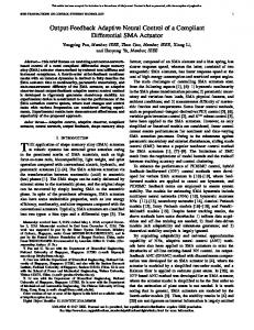
Fig. 1

E^

Output Feedback Adaptive Controller Architecture.

ˆ u) is the best available where v is commonly referred to as a pseudo control signal, and h(y, approximation of h(x, u). Then, the system dynamics can be expressed as y (r) = v + ∆,

(5)

where ˆ 1, h ˆ −1 (ξ1 , v)). ˆ −1 (ξ1 , v)) − h(ξ ∆(ξ, χ, v) = h(ξ, χ, h

(6)

ˆ u). is the difference between the possibly unknown function h(ξ, χ, u) and its estimate h(y, The pseudo control is chosen to have the form v = yc(r) + vdc − vad ,

(7)

(r)

where yc is the r-th derivative of the input signal, generated using an r-th (or higher) order stable reference model forced by an external input, vdc is dynamic compensator, and vad is the adaptive control signal designed to cancel ∆. A block diagram of the proposed controller is shown in Figure 1. ¿From (6), notice that ∆ depends on vad through v, whereas vad has to be designed to cancel ∆. Therefore the following assumption is introduced to guarantee existence and uniqueness of a solution for vad . Assumption 3.1. The map vad → ∆ is a contraction over the entire input domain of interest. Using (6), the condition in Assumption 3.1 implies:

5

ˆ ∂u ∂v ∂(h − h) ˆ ∂u ∂∆ ∂(h − h) < 1, = ∂vad = ∂u ˆ ∂v ∂vad ∂u ∂ h which can be re-written in the following way: ∂h/∂u − 1 < 1. ˆ ∂ h/∂u

(8)

(9)

Condition (9) is equivalent to:

 ˆ 1. sgn (∂h/∂u) = sgn ∂ h/∂u . ˆ 2. |∂ h/∂u| > |∂h/∂u|/2 > 0. The first condition states that unmodelled control reversal is not permissible, and the second condition places a lower bound on our estimate of the control effectiveness in (4). The input to the dynamic compensator in Figure 1 is the tracking error, which is defined by y˜ = yc − y.

(10)

ˆ ·) should be defined It is important to point out that the model approximation function h(·, so that it is invertible with respect to u, allowing the actual control input to the system to be computed by ˆ −1 (y, v). (11) u=h 3.2

Design of the Dynamic Compensator and Error Dynamics

Define the dynamic compensator as: η˙ = Ac η + bc y˜ vdc = cc η + dc y˜ , η ∈ Rr−1 . T  Then the vector e = y˜ y˜˙ · · · y˜(n−1) together with the compensator state η will the following dynamics, hereafter (with a slight abuse of language) referred to as tracking dynamics:

e e˙ b A − dc bc −bcc + = [vad − ∆] bc c Ac η η˙ 0 T ∆  y˜ η T , z = where

    A =   

1 0 ··· 0 1 .. ... . 0 0 0 0 0 ··· 0 0 .. .

  0  0      , b =     1  0

0 0 .. .



     , c = 1 0 0 ··· 0 ,  0  1

(12) obey error

(13)

6

and z is an output error signal available for use in the observer design step. For ease of notation, define the following matrices

A − d bc −bc c c A¯ = , bc c Ac b ¯ b = , 0

c 0 ¯ C = (14) 0 I and a new vector ∆

E=



e η

.

(15)

With these definitions the error dynamics (13) can be re-written as ¯ [vad − ∆] ¯ +b E˙ = AE ¯ z = CE.

(16)

Note that Ac , bc , cc , dc in (12) should be designed such that A¯ is Hurwitz. Naturally there might be multiple approaches for doing this in the most general case. Also, η needs to be at least of dimension (r − 1).

4

Design and Analysis of an Observer for the Error Dynamics

For the full state feedback application [2, 18, 20, 21], Lyapunov like stability analysis of the error dynamics in (16) results in update laws for the adaptive control parameters in terms of the error vector, E. In [10, 11, 15] adaptive state observers are used to provide the necessary estimates in the adaptation laws. However, the stability analysis was limited to second order systems with position measurements. To relax these assumptions, we propose a simple linear observer for the tracking error dynamics (16), assuming that the adaptive part of the control signal can compensate for the inversion error. This observer gives estimates of the feedback linearized states that will be used in the update laws of the adaptive parameters in Section 6. Thus, consider the following linear observer for the tracking error dynamic system in (16): ˙ Eˆ = A¯Eˆ + K (z − zˆ) ˆ zˆ = C¯ E,

(17)

where K is a gain matrix, and should be chosen such that A¯ − K C¯ is asymptotically stable, and z is defined in (16). The following remark will be useful in the sequel. Remark 4.1. Equation (17) provides estimates only for the states that are feedback linearized with the transformation (2), and not for the states that are associated with the internal dynamics.

7

This observer design ignores the nonlinearities that enter the tracking error dynamics (16) as a forcing function. This can be justified by the fact that the original nonlinear system is feedback linearized, or that vad nearly cancels ∆. This will be demonstrated in section 6 by using Lyapunov stability analysis. Let ∆ ¯ A˜ = A¯ − K C,

E˜ = Eˆ − E.

(18)

Then the observer error dynamics can be written: ¯ [vad − ∆] . E˜˙ = A˜E˜ − b

5

(19)

SHL NN Approximation of the Inversion Error

The term “artificial NN” has come to mean any architecture that has massively parallel interconnections of simple “neural” processors. Given x ∈ RN1 , a three layer-layer NN has an output given by    N N2 1   wij σ yi = vjk xk + θvj + θwi , i = 1, . . . , N3 , (20) j=1

k=1

where σ(·) is activation function, vjk are the first-to-second layer interconnection weights, and wij are the second to third layer interconnection weights. θvj and θwj are bias terms. Such an architecture is known to be a universal approximator of continuous nonlinearities with “squashing” activation functions [6, 7]. A general function f (x) ∈ C k , x ∈ D ⊂ Rn can be written as (21) f (x) = M T σ(N T x) + $(x) , where $(x) is the function reconstruction error. In general, given a constant real number $∗ > 0, f (x) is within $∗ range of the NN (20), if there exist constant weights M, N , such that for all x ∈ Rn Eq. (21) holds with $ < $∗ . Definition 5.1. The function range of NN (20) is dense over a compact set D, if for any f (·) ∈ C k and $∗ > 0, there exists a finite set of bounded weights M, N , such that (21) holds with $ < $∗ . The following theorem extends these results to map the unknown dynamics of an observable plant from available input/output history [1, 8]. Theorem 5.1. Given $∗ > 0, there exists a set of bounded weights M, N , such that ∆(ξ, χ, v) in (6) can be approximated over a compact set D ⊂ Ω × R by a single hidden layer NN (22) ∆ = M T σ(N T µ) + $(µ), $ < $∗ using the input vector

 T µ(t) = 1 v¯dT (t) y¯dT (t) ,

(23)

8

where

v¯dT (t) = [ v(t) v(t − d) · · ·

v (t − (n1 − r − 1)d) ]T

y¯dT (t) = [ y(t) y(t − d) · · ·

y (t − (n1 − 1)d)

]T

with n1 ≥ n and d > 0, σ is any squashing function. The input/output history of the original nonlinear plant is needed to map ∆ in systems with zero dynamics, because for such systems the unobservable subspace is not estimated by (17), as noted in Remark 4.1. If the system has full relative degree, the observer in (17) provides all the estimates needed for the reconstruction of ∆, and no past input/output history is required [9]. The adaptive term in (7) is designed as: ∆ ˆT ˆ T µ), σ(N vad = M

(24)

ˆ and N ˆ are the NN weights to be updated on line. With squashing functions, the where M equation (24) will always have at least one fixed point solution. Using (22) the error dynamics can be expressed as:   ¯ M ˆ T µ) − M T σ(N T µ) − $ ¯ +b ˆ T σ(N E˙ = AE ¯ z = CE.

(25)

Define

˜ =M ˆ − M, N ˜ =N ˆ −N, M

Z˜ =

˜ 0 M ˜ 0 N

,

(26)

and note that: ˆ F < M ˜ F + M ∗ , M

ˆ F < N ˜ F + N ∗ , N

(27)

where M ∗ , N ∗ are the upper bounds for the weights in (22): M F < M ∗ ,

N F < N ∗ ,

(28)

the subscript F denoting the Frobenius norm. With (27), the representation ˆ T σ(N ˆ T µ) − M T σ(N T µ) − $ vad − ∆ = M

(29)

allows for the following upper bound for some computable α1 , α2 : ˜ F + α2 , vad − ∆ ≤ α1 Z

α1 > 0,

α2 > 0.

(30)

For the stability proof we will need the following representation: 

ˆTµ + M ˜Tµ + w , ˆ T σ(N ˆ T µ) − M T σ(N T µ) = M ˜T σ ˆ Tσ M ˆN ˆ−σ ˆN ˆ µ), where σ ˆ = σ(N ˜ T µ)2 . ˜ Tσ ˆ  N T µ − M T O(N w=M Such a representation is achieved via Taylor series expansion of σ(N T µ) around the estimates ˆ T µ (refer to [18] for more details). The following assumption is used in the stability analysis. N

9

Assumption 5.1. Assume that the input vector to the NN is uniformly bounded: µ ≤ µ∗ ,

µ∗ > 0.

(31)

A similar assumption is made in [4]. With (31) a bound over the compact set D for (w − $) can be presented as follows [18]: ˜ F + γ2 , w − $ ≤ γ1 Z

γ1 > 0,

γ2 > 0 ,

(32)

where γ1 , γ2 are computable constants, and γ1 comprises the unknown constant µ∗ , γ2 comprises the $∗ . Thus the forcing term in (25) can be written:

 ˆTµ + M ˜ T µ + w − $, ˜T σ ˆ Tσ vad − ∆ = M ˆ−σ ˆN ˆN (33) subject to (31), (32).

6

Stability Analysis

The stability analysis of the closed-loop system should be done taking into account the observer error dynamics. We will prove ultimate boundedness of the error signals of the following system: ¯ [vad − ∆] ¯ +b E˙ = AE ¯ [vad − ∆] . E˜˙ = A˜E˜ − b

(34)

The following two lemmas are useful in the sequel: ˆ , W0 be matrices in Rn×m , and Lemma 6.1. Let W , W ∆ ˆ ˜ = W W − W.

Then the following is true:   ˜ T (W ˆ − W0 ) = 1 W ˜ 2 + 1 W ˆ − W0 2 − 1 W − W0 2 . tr W F F F 2 2 2 Proof: The result follows by using AF = trAT A and some basic properties of matrices. Lemma 6.2. [14] If A is an asymptotically stable matrix, then given any positive definite symmetric matrix Q  0, there exists a unique positive definite symmetric matrix P  0 such that AT P + P A = −Q

(35)

10

Theorem 6.1. Let assumptions 2.1, 3.1 hold. Consider the following weight adaptation laws:   ¯M ˆ˙ = −G 2µEˆ T P b ˆ Tσ ˆ − N0 ) N ˆ  + k(N (36)   ¯ + k(M ˆ˙ = −F 2(ˆ ˆ T µ)Eˆ T P b ˆ − M0 ) M σ−σ ˆN (37)   ∆ ¯ 2 , where κ1 = Θα1 + P bγ ¯ 1, Θ = ¯ + P˜ b||, ¯ and P, P˜ P b for F, G  0, k > 2 κ21 + γ12 P b satisfy: ˜ A˜T P˜ + P˜ A˜ = −Q, A¯T P + P A¯ = −Q, ˜ > 1. Then the feedback control law given by ˜ Q  0 with λmin (Q) > 1, λmin (Q) for some Q, ˆ −1 (y, v), u=h where v = yc(r) + vdc − vad vdc = Cc η + Dc y˜ ˆ T σ(N ˆ T µ) vad = M

(38)

˜ M ˜,N ˜ in the closed loop system are ultimately bounded, proguarantees that all signals E, E, vided D is sufficiently large. Proof: Consider the following Lyapunov function candidate: 1 ˜ ) + 1 tr(N ˜ ), ˜ T F −1 M ˜ T G−1 N V = E T P E + E˜ T P˜ E˜ + tr(M 2 2 The derivative of V along (34) will be V˙

  ¯ vad − ∆ ˜ E˜ + 2E T P b = −E T QE − E˜ T Q   T ˜¯ ˜˙ ) + tr(N ˜ T G−1 N ˜˙ ). ˜ T F −1 M ˜ −2E P b vad − ∆ + tr(M

With the definition of E˜ = Eˆ − E and (33), this can be written:

  ¯ M ˜ E˜ + 2Eˆ T P b ˆTµ + M ˜ T µ + w − $] ˆ Tσ ˜T σ V˙ = −E T QE − E˜ T Q ˆ−σ ˆN ˆN   T ˜¯ ¯ ˜˙ ) + tr(N ˜ T G−1 N ˜˙ ). ˜ T F −1 M ˜ −2E (P b + P b) vad − ∆ + tr(M Substituting the adaptive laws implies: V˙

 T ˜ ˜ T ¯ ˆ ˜ = −E QE − E QE + 2E P b w − $]   ¯ + P b) ¯ vad − ∆ −2E˜ T (P˜ b     ˜ (N ˆ − N0 ) . ˜ (M ˆ − M0 ) − ktr N −ktr M T

(39)

11

Using Lemma 6.1, upper bounds from (30) and (32), the derivative of the Lyapunov function candidate can be upper bounded as: V˙

˜ E ˜ 2 ≤ −λmin (Q)E2 − λmin (Q)     ¯ ˆ ˜ ˜ ˜ +2P bE γ1 ZF + γ2 + 2ΘE α1 ZF + α2 k ˆ k k ˜ 2 F − M − M0 2F + M − M0 2F − − M 2 2 2 k ˆ k k ˜ 2 − N F − N − N0 2F + N − N0 2F . 2 2 2

(40)

Further V˙

˜ E ˜ 2 ≤ −λmin (Q)E2 − λmin (Q)     ¯ ˜ α1 Z ˜ ˜ F + γ2 + 2ΘE ˜ F + α2 +2P b(E + ||E||) γ1 Z k ˜ 2 ¯ − Z F + Z, 2

(41)

where  k ∆ M − M0 2F + N − N0 2F . Z¯ = 2

(42)

Grouping terms, (41) can be written: V˙

˜ E ˜ 2 ≤ −λmin (Q)E2 − λmin (Q)  



  ¯ γ1 Z ¯ ˜ Θ α1 Z ˜ F + γ2 + 2E ˜ F + α2 + P b ˜ F + γ2 +2P bE γ1 Z k ˜ 2 ¯ − Z F + Z, 2

(43)

and further put in the form: V˙

˜ E ˜ 2 ≤ −λmin (Q)E2 − λmin (Q)     ¯ ˜ ˜ ˜ +2P bE γ1 ZF + γ2 + 2E κ1 ZF + κ2 k ˜ 2 ¯ − Z F + Z, 2

(44)

¯ 2 . Upon completion of squares, we get: where κ2 = Θα2 + P bγ   ¯ V˙ ≤ −E (λmin (Q) − 1) E − 2γ2 P b   

˜ ˜ ˜ −E λmin (Q) − 1 E − 2κ2  2 ˜ − κ1 Z ˜ F + κ21 Z ˜ 2F − E 2    ¯ Z ˜ F + γ1 P B ¯ 2 Z ˜ 2F − E − γ1 P b k ˜ 2 ¯ − Z F + Z, 2

(45)

12

which further allows for the following upper bound:   ¯ V˙ ≤ −E (λmin (Q) − 1) E − 2γ2 P b  

 ˜ ˜ ˜ −E λmin (Q) − 1 E − 2κ2  

 2 k 2 2 ¯ ˜ ¯ ZF − Z . − − κ1 − γ1 P b 2

(46)

The following conditions ¯ 2 2P bγ λmin (Q) − 1 2κ2 ˜ > E ˜ −1 λmin (Q)  Z¯ ˜ F > Z   k 2 ¯ 2 − κ − γ P b 1 1 2 E >

(47)

will render V˙ < 0 outside a compact set. To ensure, that the conditions (47) define a compact set in the space of error variables, introduce the following notations: ¯ 2 2P bγ λmin (Q) − 1 2κ2 β2 = ˜ −1 λmin (Q)  Z¯ β3 =   k ¯ 2 − κ21 − γ1 P b 2 Υ = Z¯ + β12 + β22 β1 =

(48)

and write (46) in the following way: 2

2 ˙ ˜ ˜ 2+Υ V ≤ − (E − β1 ) − E − β2 − β3 Z

(49)

¿From (49), it follows, that the condition V˙ < 0 is true everywhere in the space of error variables ˜ Z, ˜ outside the ellipsoid: E, E,

2 2 ˜ ˜ 2=Υ (E − β1 ) + E − β2 + β3 Z (50) which is a compact set that touches the origin. To conclude ultimate boundedness one must define the set of possible initial conditions for the error variables and ensure that this set is an invariant set, including the origin. Introduce the compact sets: Bc = {yc | yc  ≤ bc }

(51)

13

Br

r Ωβ Ωα

Fig. 2

Geometric Representation of the Sets in the Error Space.

and BZ = {vecZ | vecZ ≤ bZ } where

Z=

Consider the vector

M 0 0 N

(52)

.

(53)



 E ζ =  E˜  , vecZ˜

and define the compact set ∆

Br = {ζ | ζ ≤ r},

(54)

for a given r > C. The value of C will be specified in the sequel. Consider the Lyapunov function candidate in (39). Let α be the minimum value of the Lyapunov function V on the edge of Br : ∆

α = min V.

(55)

Ωα = {ζ ∈ Br | V ≤ α}.

(56)

ζ=r

Define

This and all other sets defined in this analysis are represented graphically in Figure 2. We have proven that the derivative of the Lyapunov function candidate (39) is negative definite for ∆

ζ ≥ max(β1 , β2 , β3 ) = C,

14

which implies that for the domain Ωβ = {ζ ∈ Br | z < C}

(57)

the derivative is sign indefinite. We need to ensure Ωβ ⊂ Ωα , making Ωα a positive invariant set. This requirement implies an upper bound to the adaptation gains F and G in Theorem 6.1. Based on above notations our choice of Lyapunov function can be represented as: V = ζ T T ζ, where 

 P 0 0 0 ˜ 0 0  ∆ 1 0 P . T =  2  0 0 F −1 0  0 0 0 G−1

(58)

Then α is: ∆

α = min ζ T T ζ = r2 Tm , ζ=r

(59)

where Tm is the minimum singular value of T . The requirement that Ωβ ⊂ Ωα imposes the following condition on Tm : Tm >

C . r2

(60)

This condition can be met by appropriate choice of the parameters in (58). For example, the condition (60) can be viewed in terms of learning rates once the linear design is fixed. If F = γF I, G = γG I, then the minimum singular value is determined by the learning rates γF−1 , γG−1 . Let ∆ γm = max(γF , γG ). Then the condition (60) yields: γm