Advanced Control Algorithms for Compact and Highly ...

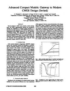
Advanced Control Algorithms for Compact and Highly Efficient Displacement-Controlled Multi-Actuator and Hydraulic Hybrid Systems Enrique Busquets Pump Switching pressure (bar)

Precision Motion Control position (°)

100 75 50 25 0

4

6

8

10

12

200 150 100 50 0 185

14

190

195

time (s)

time (s)

Engine Power Management 550 500 450

60

400 350

40

300 20 250 1500

2000

2500

200

ne (rpm)

1.00 0.75 0.50 0.25 0 0 75 0 100 200 150

dp (bar)

n (rpm)

Anti-Stall Control

West Lafayette 2016

php (bar)

0

SA (-)

Me (Nm)

80

350 300 250 200

0

5

10

15

20

time (s)

Hydraulic Hybrid Power Management

i

ADVANCED CONTROL ALGORITHMS FOR COMPACT AND HIGHLY EFFICIENT DISPLACEMENT-CONTROLLED MULTI-ACTUATOR AND HYDRAULIC HYBRID SYSTEMS

A Dissertation Submitted to the Faculty of Purdue University by Enrique Busquets

In Partial Fulfillment of the Requirements for the Degree of Doctor of Philosophy

August 2016 Purdue University West Lafayette, Indiana

ii

For my family

iii

ACKNOWLEDGEMENTS

There are a number of people whom I would like to thank for being part of my life during the course of these past years. First and foremost I would like to thank my family whose support made this achievement possible. I must also thank my advisor Prof. Monika Ivantysynova for her support, guidance and expert advice throughout this journey. Finally, I would like to acknowledge my fellow researchers from the Maha Fluid Power Research Center as well as Anthony Franklyn for the many hours spent working at the lab. My especial gratitude goes to Josh Zimmerman for providing the guidance and great advice as a graduate mentor during the summer of 2010 as well as a colleague and friend during the past years.

iv

TABLE OF CONTENTS

Page LIST OF TABLES ................................................................................................ viii LIST OF FIGURES ................................................................................................ ix NOMENCLATURE.............................................................................................. xvii ABSTRACT ........................................................................................................ xxiii CHAPTER 1.

INTRODUCTION...................................................................... 1

1.1

Background ..................................................................................................1

1.2

Pump Switching............................................................................................3

1.3

Secondary-Control .......................................................................................4

1.4

1.3.1

Displacement Control with Secondary-Controlled Hydraulic Hybrid

Drives

....................................................................................................... 5

Dissertation Organization .............................................................................7

CHAPTER 2.

STATE OF THE ART ............................................................... 9

2.1

Advanced control Algorithms for Valve-Controlled Actuation ................... 10

2.2

Throttle-Less Actuation Systems and Control Advancements .................. 14 2.2.1

Electro-Hydraulic Actuation Controls ........................................... 14

2.2.2

Displacement-Controlled Actuation and Controls ........................ 16

2.2.3

Secondary-Controlled Actuation Controls and their Role in

Hydraulic Hybrids ......................................................................................... 24 CHAPTER 3.

EXPERIMENTAL

PLATFORMS’

DYNAMIC

MODELING,

SIMULATION AND VALIDATION THROUGH MEASUREMENTS ..................... 29 3.1

Joint Integrated Rotary Actuation System for Pump Switching ................ 29 3.1.1 3.1.1.1

Mechanical and Hydraulic Systems’ Mathematical Models ......... 31 Axial Piston Machine Model ..................................................... 31

v

Page

3.2

3.1.1.2

Linear Actuator Model .............................................................. 33

3.1.1.3

Hydraulic Rotary Actuator Dynamic Model .............................. 34

3.1.1.4

Switching Valves Model ........................................................... 35

3.1.2

Joint Integrated Rotary Actuation Measurement Setup ............... 35

3.1.3

Step Command Measurement ..................................................... 37

Displacement-Controlled Hydraulic Hybrid Excavator Prototype .............. 40 3.2.1

Excavator Mechanical and Hydraulic Mathematical Models ........ 43

3.2.1.1

Hydraulic Hybrid Swing Drive Model ....................................... 44

3.2.1.2

Hydraulic Hybrid Swing Drive Reduced-Order Model ............. 46

3.2.1.3

Low Pressure System Model ................................................... 46

3.2.1.4

Mechanical System Model ....................................................... 48

3.2.1.5

Prime Mover Model .................................................................. 50

3.2.1.6

Excavator Baseline Controller ................................................. 51

3.2.2

Excavator Measurement Setup .................................................... 53

3.2.3

Excavator Model Validation Measurements ................................. 56

CHAPTER 4. 4.1

CONTROL SYNTHESIS ........................................................ 61

Actuator-Level Controls for DC and Secondary-Controlled Actuators ...... 61 4.1.1

Adaptive Robust Control for Displacement-Controlled Actuators 62

4.1.1.1

Nonlinear Controller Synthesis ................................................ 64

4.1.1.1.1

ARC Controller Design Step 1 ........................................... 66

4.1.1.1.2


4.1.1.1.3


4.1.1.2

Controller Assumptions ............................................................ 71

4.1.1.3

Controller Parameters .............................................................. 72

4.1.2

Actuator Level Control for Secondary-Controlled Hybrid Drives .. 73

4.1.2.1 4.1.2.1.1 4.1.2.2

Baseline Controller ................................................................... 74 Baseline Controller Parameters ......................................... 74 Robust H∞ Multi-Input Multi-Output Controller ......................... 74

4.1.2.2.1

H∞ Controller Design Step 1 .............................................. 75

4.1.2.2.2


vi

Page 4.1.2.2.3 4.1.2.3 4.1.3

Adaptive Robust Controller Synthesis ..................................... 82 Control Strategies for Pump Switching on the Actuator Level ..... 84

4.1.3.1

Pump Dynamics ....................................................................... 85

4.1.3.1.1 4.1.3.2 4.2


Incorrect Pilot-Operated Check Valves Opening ............... 86 Flow Summing Transitions....................................................... 87

Supervisory Level Control Strategies for Pump Switching and Hydraulic

Hybrid Multi-Actuator Systems ............................................................................ 89 4.2.1

Priority-Based Supervisory Controller for Pump Switching .......... 90

4.2.1.1 4.2.2

Supervisory Controller Parameters .......................................... 97 Supervisory Controller for the Power Management of Hydraulic

Hybrid Multi-Actuator Systems .................................................................... 97 4.2.2.1

The Engine Power Management Control Strategy .................. 97

4.2.2.1.1

The Engine Anti-Stall Controller ........................................ 98

4.2.2.2

Primary Unit Feedforward Control ......................................... 103

CHAPTER 5.

CONTROLLER MEASUREMENT RESULTS ...................... 107

5.1

Actuator-Level Controls Experimental Results ....................................... 107 5.1.1

Adaptive Robust Control for DC Actuators ................................ 107

5.1.1.1

Sinusoid Command ................................................................ 108

5.1.1.2

Rate-limited Step Command .................................................. 110

5.1.2

Hydraulic Hybrid Actuator-Level Control Measurement Results 113

5.1.2.1

0° ~ 90° Swing Command...................................................... 115

5.1.2.1.1

Low Inertia Case .............................................................. 115

5.1.2.1.2

High Inertia Case ............................................................. 119

5.1.2.2

0° ~ 180° swing command ..................................................... 123

5.1.2.2.1

Low Inertia Case .............................................................. 123

5.1.2.2.2

High Inertia Case ............................................................. 127

5.1.3

Pump Switching Measurement Results on the Actuator Level .. 132

5.1.3.1

Measurements on the JIRA Test Bench ................................ 132

5.1.3.2

Measurements on the Excavator Prototype ........................... 141

vii

Page 5.2

Supervisory-Level Controls Experimental Validation .............................. 147 5.2.1

Pump Switching Supervisory Controller Measurement Results 147

5.2.1.1

Single Actuator Operation ...................................................... 147

5.2.1.2

Conflicting Actuator Combinations ......................................... 149

5.2.1.3

Trench Digging Cycle ............................................................. 150

5.2.2

Power Management Supervisory Control Measurements ......... 154

5.2.2.1

Measurements of the Anti-Stall Controller ............................. 154

5.2.2.2

Hydraulic Hybrid Power Management Controller Measurements ............................................................................................... 157

CHAPTER 6.

CONCLUSIONS AND FUTURE WORK .............................. 163

BIBLIOGRAPHY ................................................................................................ 167 VITA ................................................................................................................... 179 PUBLICATIONS ................................................................................................ 181

viii

LIST OF TABLES

Table ................................................................................................................ Page Table 1: Joint integrated rotary actuation sensor information ............................. 37 Table 2: Joint integrated rotary actuation DAQ and control information ............. 37 Table 3: Structural components geometrical dimensions.................................... 49 Table 4: Center of gravity coordinates and mass properties ............................... 49 Table 5: Excavator DAQ and control information ................................................ 55 Table 6: Excavator sensor information ................................................................ 55 Table 7: Calculated parameter bounds ............................................................... 72 Table 8: Uncertain parameter ranges for the design of the H∞ controller ........... 76 Table 9: Modified uncertain parameter ranges to study the baseline control...... 82 Table 10: Excavator actuator truth table.............................................................. 92

ix

LIST OF FIGURES

Figure ............................................................................................................... Page Figure 1: Displacement-controlled actuator hydraulic circuit ................................. 2 Figure 2: Low pressure system architecture.......................................................... 3 Figure 3: Displacement-controlled actuator with pump switching hydraulic circuit 4 Figure 4: Secondary-controlled actuators hydraulic circuit.................................... 5 Figure 5: Secondary-controlled actuators with energy storage hydraulic circuit ... 5 Figure 6: Displacement-controlled actuation with a secondary-controlled hydraulic hybrid drive ............................................................................................................ 6 Figure 7: Electro-hydraulic actuator hydraulic circuit ........................................... 15 Figure 8: Open-circuit DC actuation .................................................................... 17 Figure 9: Displacement-controlled actuator hydraulic circuit ............................... 18 Figure 10: Displacement-controlled multi-actuator system hydraulic circuit ....... 20 Figure 11: Representative DC system with pump switching with three actuators ............................................................................................................................. 20 Figure 12: DC excavator prototype system proposed by Zimmermann (Zimmermann, 2009) ........................................................................................... 23 Figure 13: Proposed test bench hydraulic circuit ................................................ 30 Figure 14: Proposed test bench mechanical system ........................................... 31

x

Figure ............................................................................................................... Page Figure 15: Hydraulic unit four-quadrant operation for a given unit speed ........... 32 Figure 16: Joint integrated rotary actuation hardware system ............................ 36 Figure 17: Joint integrated rotary actuation system data acquisition and control 36 Figure 18: Rotary actuator measured and simulated pressures ......................... 38 Figure 19: Rotary actuator measured and simulated position ............................. 38 Figure 20: Rotary actuator measured and simulated velocity ............................. 38 Figure 21: Linear actuator measured and simulated pressures .......................... 39 Figure 22: Actuator simulated position ................................................................ 39 Figure 23: Actuator simulated velocity................................................................. 39 Figure 24: Measured normalized displacement command.................................. 40 Figure 25: Displacement-controlled excavator prototype with a secondarycontrolled hydraulic hybrid swing drive and pump switching ............................... 42 Figure 26: Multi-body dynamic and hydraulic systems co-simulation structure .. 44 Figure 27: Free-body diagrams of the excavator top and side views .................. 45 Figure 28: Volumetric efficiency .......................................................................... 47 Figure 29: Mechanical efficiency ......................................................................... 47 Figure 30: Pilot-operated check valve cross-sectional view ................................ 48 Figure 31: Excavator components physical dimensions ..................................... 49 Figure 32: Diesel engine scaled WOT curve ....................................................... 50 Figure 33: Feedforward actuator-level baseline controller for DC actuators ....... 52 Figure 34: Secondary-controlled hydraulic hybrid baseline controller ................. 53 Figure 35: Excavator prototype and working hydraulics ...................................... 53 Figure 36: Compact excavator system data acquisition and control ................... 54

xi

Figure ............................................................................................................... Page Figure 37: Prime mover measured and simulated rotational speed .................... 56 Figure 38: Actuator measured and simulated positions ...................................... 58 Figure 39: Actuator measured and differential pressures ................................... 59 Figure 40: Displacement-controlled multi-actuator machine controller with pump switching and hybrid drives ................................................................................. 61 Figure 41: Simplified JIRA DC rotary actuator hydraulic circuit .......................... 63 Figure 42: Adaptive robust control block diagram for a first-order system .......... 65 Figure 43: Excavator hydraulic hybrid swing drive .............................................. 73 Figure 44: Nominal open-loop plant and desired loop-shaped singular values .. 76 Figure 45: H∞ controller structure ........................................................................ 77 Figure 46: General control configuration for control study .................................. 78 Figure 47: N∆-structure ........................................................................................ 78 Figure 48: M∆-structure ....................................................................................... 78 Figure 49: Structured Singular Values of the M matrix with the H∞ controller ..... 79 Figure 50: Structured Singular Values of the N matrix with the H∞ controller ..... 80 Figure 51: Structured Singular Values of the M matrix with the baseline controller ............................................................................................................................. 81 Figure 52: Structured Singular Values of the N matrix with the baseline controller ............................................................................................................................. 81 Figure 53: Flow summing control strategy........................................................... 88 Figure 54: Proposed priority-based controller scheme........................................ 94 Figure 55: Combination indexing algorithm flowchart ......................................... 96 Figure 56: Proposed anti-stall controller framework .......................................... 100

xii

Figure ............................................................................................................... Page Figure 57: Rule-based operating mode predictor flowchart .............................. 100 Figure 58: Manually tuned anti-stall gain schedule ........................................... 101 Figure 59: Hydraulic hybrid multi-actuator system power distribution ............... 103 Figure 60: Actuator trajectory for the sinusoid command .................................. 108 Figure 61: Actuator position error, e1 ................................................................. 108 Figure 62: Actuator velocity error, e2.................................................................. 109 Figure 63: Actuator virtual torque input error, e3 ................................................ 109 Figure 64: Normalized control effort for the sinusoid command ........................ 109 Figure 65: Actuator pressures for the sinusoid command ................................. 110 Figure 66: Normalized parameter estimates for the sinusoid command ........... 110 Figure 67: Actuator trajectory for the rate-limited step command ..................... 110 Figure 68: Actuator position error, e1 ................................................................. 111 Figure 69: Actuator velocity error, e2.................................................................. 111 Figure 70: Actuator virtual torque input error, e3 ................................................ 111 Figure 71: Normalized control effort for the rate-limited step command ........... 112 Figure 72: Actuator pressures for the rate-limited step command .................... 112 Figure 73: Normalized parameter estimates for the rate-limited step command ........................................................................................................................... 112 Figure 74: Measured artificial and expert operator joystick commands ............ 114 Figure 75: Excavator cabin position for the 0 ~ 90° truck loading cycle with low inertia and the three proposed controllers ......................................................... 116 Figure 76: Excavator cabin velocity for the 0 ~ 90° truck loading cycle with low inertia and the three proposed controllers ......................................................... 117

xiii

Figure ............................................................................................................... Page Figure 77: Excavator cabin position and velocity errors for the 0 ~ 90° truck loading cycle with low inertia and the three proposed controllers .................................. 118 Figure 78: Control effort for the 0 ~ 90° truck loading cycle with low inertia and the three proposed controllers ................................................................................. 118 Figure 79: Secondary-controlled accumulator state-of-charge for the 0 ~ 90° truck loading cycle with low inertia and the three proposed controllers ..................... 119 Figure 80: Excavator cabin position for the 0 ~ 90° truck loading cycle with high inertia and the three proposed controllers ......................................................... 120 Figure 81: Excavator cabin velocity for the 0 ~ 90° truck loading cycle with high inertia and the three proposed controllers ......................................................... 121 Figure 82: Excavator cabin position and velocity errors for the 0 ~ 90° truck loading cycle with high inertia and the three proposed controllers ................................ 122 Figure 83: Control effort for the 0 ~ 90° truck loading cycle with high inertia and the three proposed controllers ................................................................................. 122 Figure 84: Secondary-controlled accumulator state-of-charge for the 0 ~ 90° truck loading cycle with high inertia and the three proposed controllers .................... 123 Figure 85: Excavator cabin position for the 0 ~ 180° truck loading cycle with low inertia and the three proposed controllers ......................................................... 124 Figure 86: Excavator cabin velocity for the 0 ~ 180° truck loading cycle with low inertia and the three proposed controllers ......................................................... 125 Figure 87: Excavator cabin position and velocity errors for the 0 ~ 180° truck loading cycle with low inertia and the three proposed controllers ..................... 126

xiv

Figure ............................................................................................................... Page Figure 88: Control effort for the 0 ~ 180° truck loading cycle with low inertia and the three proposed controllers ........................................................................... 126 Figure 89: Secondary-controlled accumulator state-of-charge for the 0 ~ 90° truck loading cycle with high inertia and the three proposed controllers .................... 127 Figure 90: Excavator cabin position for the 0 ~ 180° truck loading cycle with high inertia and the three proposed controllers ......................................................... 128 Figure 91: Excavator cabin velocity for the 0 ~ 180° truck loading cycle with high inertia and the three proposed controllers ......................................................... 129 Figure 92: Excavator cabin position and velocity errors for the 0 ~ 180° truck loading cycle with high inertia and the three proposed controllers .................... 130 Figure 93: Control effort for the 0 ~ 180° truck loading cycle with high inertia and the three proposed controllers ........................................................................... 130 Figure 94: Secondary-controlled accumulator state-of-charge for the 0 ~ 90° truck loading cycle with high inertia and the three proposed controllers .................... 131 Figure 95: Actuator normalized positions .......................................................... 131 Figure 96: Excavator cabin parameter estimate related to cabin inertia ........... 132 Figure 97: Measured relevant parameters for the evaluation of pump switching with 125ms switching time ........................................................................................ 135 Figure 98: Measured relevant parameters for the evaluation of pump switching with 250ms switching time ........................................................................................ 136 Figure 99: Measured relevant parameters for the evaluation of pump switching with 500ms switching time ........................................................................................ 137

xv

Figure ............................................................................................................... Page Figure 100: Multiple pump switching events for a large load of the rotary actuator ........................................................................................................................... 139 Figure 101: Normalized measured hydraulic units’ displacements ................... 140 Figure 102: Rotary actuator velocity .................................................................. 140 Figure 103: Pump switching demonstration without control using the boom actuator under a large load .............................................................................................. 143 Figure 104: Pump switching demonstration with control using the boom actuator under a large load .............................................................................................. 144 Figure 105: Pump switching demonstration without control using the boom actuator under a small load ............................................................................................. 145 Figure 106: Pump switching demonstration with control using the boom actuator under a small load ............................................................................................. 146 Figure 107: Supervisory controller evaluation for single-actuator usage .......... 148 Figure 108: Supervisory controller output for three actuator combination conflicts due to architecture constraints .......................................................................... 150 Figure 109: Actuator positions for the trench-digging cycle .............................. 151 Figure 110: Supervisory controller output for the trench-digging cycle ............. 152 Figure 111: Hydraulic units providing flow for the commanded motion ............. 152 Figure 112: Corresponding switching valves for the trench-digging cycle ........ 152 Figure 113: Hydraulic units’ measured differential pressures ........................... 155 Figure 114: Calculated resulting engine torque load ......................................... 155 Figure 115: Unit 1 displacements before and after the anti-stall control .......... 156 Figure 116: Unit 2 displacements before and after the anti-stall control .......... 156

xvi

Figure ............................................................................................................... Page Figure 117: Unit 3 displacements before and after the anti-stall control .......... 156 Figure 118: Unit 4 displacements before and after the anti-stall control .......... 157 Figure 119: Measured engine speed error ........................................................ 157 Figure 120: Calculated machine Power distribution .......................................... 158 Figure 121: Measured primary unit displacement ............................................. 159 Figure 122: Measured hydraulic hybrid accumulator state-of-charge ............... 159 Figure 123: Measured engine speed ................................................................. 160 Figure 124: Engine operation during the measured cycle ................................. 160

xvii

NOMENCLATURE

Symbol

Description

Units

d

External disturbance force

N

dPO

Pilot-operated check valve spool diameter

N

ds

Switching valve valve spool diameter

N

e1 … en

State errors

-

e1 … en

State error dynamics

-

f

Lumped external and hard-to-model forces

N

fs

Static friction coefficient

N

fc

Coulomb friction coefficient

N

fv

Viscous friction coefficient

kg/s

g

Gravity

m/s2

iTOT

Total gear ratio

-

k

Spring stiffness coefficient

N/m

k1… kn

Linear gains

-

k1r1… knr1

Robust control linear stabilizing gains

-

kL

Pressure-dependent volumetric flow losses

m3/s/Pa

kv

Velocity dependent internal volumetric flow losses

m

lcg

Distance to center of gravity

m

m

Mass

kg

meq

Equivalent mass

kg

n

Rotational speed

rpm

n1

Primary unit rotational speed

rpm

ncp

Charge pump rotational speed

rpm

xviii

Symbol

Description

Units

nE

Prime mover rotational speed

rpm

p1, p2

Ports 1 and 2 pressures

bar

php

High pressure line pressure

bar

plp

Low pressure line pressure

bar

pme

Mean effective pressure

bar

po

Accumulator pre-charge pressure

bar

psetting

Relief valve pressure setting

bar

rPO

Pilot-operated check valve pilot ratio

-

rv

Viscous friction coefficient

kg/s

t

Time

s

u1, u2

Primary and secondary unit normalized commands

-

ucmd

Actuator command vector

-

u

Normalized hydraulic unit displacement command

-

uE

Prime mover normalized speed command

-

w

Weight

kg

wRTR

Right track weight factor

-

wLTR

Left track weight factor

-

wswing

Swing weight factor

-

wboom

Boom weight factor

-

warm

Arm weight factor

-

wbucket

Bucket weight factor

-

woffset

Offset weight factor

-

wblade

Blade weight factor

-

w1… wn

Adaptive controller weighting factors

-

x

Linear actuator position

m

x

Linear actuator velocity

m/s

x

Linear actuator acceleration

m/s2

xact

Actual linear actuator position

m

xarm

Arm length

m

xix

Symbol

Description

Units

xboom

Boom length

m

xbucket

Bucket length

m

xmax

Maximum actuator displacement

m

y1, y2

Valve spool displacements

m

y1 normal

PO valve spool displacement on the normal direction

m

y1 opposite

PO valve spool displacement on the opposite direction

m

ys

Switching valve spool displacement

m

A1, A2

Actuator piston and rod side areas

m2

Acc

Control cylinder area

m2

APO

Pilot-operated check valve spool area

m2

CH

Hydraulic capacitance

Pa

CH hp

High pressure line hydraulic capacitance

Pa

CH lp

Low pressure line hydraulic capacitance

Pa

Cr

Relief valve linear flow gain

m3/Pa/s

Cθ1… Cθn

Positive-definite constant diagonal matrices

-

Cφ1… Cφn

Positive-definite constant diagonal matrices

-

D

Hydraulic transmission line length

m

Fcrack

Cracking force

N

Ff

Friction force

N

Fext

External forces

N

J

Inertia

kg m2

JE

Prime mover inertia

kg m2

Jeq

Equivalent inertia

kg m2

K

Hydraulic fluid bulk modulus

Pa

Kp

Controller proportional gain

-

Ki

Controller integral gain

-

Kβ

Swash plate dynamics gain

-

L

Hydraulic transmission line length

m

Lcc

Control cylinder height

m

xx

Symbol

Description

Units

KL

Pressure-dependent Hydraulic motor internal losses

m3/Pa/s

KQ

Volumetric flow coefficient

-

KT

Torque loss coefficient

-

Ks

Stabilizing controller gain matrix

-

Kv

Control valve DC gain

-

Kβ

Swash plate DC gain

-

Kϕ

Velocity-dependent Hydraulic motor internal losses

m2

M

Torque

Nm

Mc

Coulomb friction torque

Nm

ME eff

Prime mover effective torque

Nm

ME f

Prime mover friction torque

Nm

ME th

Prime mover theoretical torque output

Nm

Mext

External torque load

Nm

Mf

Friction torque

Nm

Mi

Torque due to cabin inclination

Nm

ML

Prime mover torque load

Nm

Mm

Hydraulic motor torque output

Nm

Ms

Torque loss

Nm

MWOT

Prime mover wide-open-throttle torque

Nm

N

Polytrophic exponent

-

P

Generalized plant matrix

-

Q 1, Q 2

Ports 1 and 2 volumetric flow rates

m3/s

Q1e, Q2e

Ports 1 and 2 effective volumetric flow rates

m3/s

QAe, m, QBe, m

Effective motor volumetric flows at port A and B

m3/s

QAe, p, QBe, p

Effective pump volumetric flows at port A and B

m3/s

Qchk 1, Qchk 2

Check valves volumetric flow rates in line 1 and 2

m3/s

Qcp

Charge pump volumetric flow rate

m3/s

Qe

Effective pump flow rate

m3/s

QL, 1, QL, 2

Internal volumetric flow loss rates in line 1 and 2

m3/s

Qr1, Qr2

Relief valves volumetric flow rates

m3/s

xxi

Symbol

Description

Units

Qr lp

Low pressure relief valve volumetric flow rate

m3/s

Qs

Volumetric flow loss

m3/s

Qs, u1, Qs, u2

Primary and secondary units’ external flow losses

m3/s

Qswitching

Switching valve flow

m3/s

Qv

Control valve volumetric flow

m3/s

Sc

Scaling factor

-

Sp

Prime mover piston speed

m/s

T

Temperature

°C

V1… Vn

Adaptive controller Lyapunov functions

-

Vcc

Control cylinder volume

m3

Vcp

Charge pump volumetric displacement

cm3/rev

Vd

Derived volumetric displacement

cm3/rev

Vdead

Dead volume

m3

VL1, VL2

Hydraulic fluid volume in lines 1 and 2

m3

VL

Total hydraulic transmission line volume

m3

VM

Hydraulic motor volumetric displacement

cm3/rev

Veng

Prime mover volumetric displacement

m3

Vo

Accumulator gas volume

m3

Vu1, Vu2

Hydraulic units’ volumetric displacement

cm3/rev

W1

Glover-McFarlane pre-filter

-

α

Inclination angle

°

α1…αn

Adaptive control laws

-

α1r…αnr

Robust control laws

-

β

Hydraulic unit displacement

%

βnorm

Normalized hydraulic unit displacement

-

βjoy

Normalized joystick feedforward command

-

βref

Normalized reference displacement command

-

βu1, βu2

Hydraulic units’ displacements

-

Γ

Adaptive controller parameter adaptation rate matrix

-

Δp

Differential pressure

bar

xxii

Symbol

Description

Units

Δpact

Actual differential pressure

bar

ε

Adaptive control design parameter

-

η

Efficiency

-



Angular position

°



Angular velocity

°/s



Angular acceleration

°/s2

ˆ 1… ˆ n

Adaptive controller parameter estimates

-

 1… 

Adaptive controller parameter estimate errors

-

 1 … n

Adaptive controller parameters true values

-

 1min,  2min

Minimum parameter estimate bounds

-

 1max,  2max

Maximum parameter estimate bounds

-

 min,  max

Minimum and maximum parameter estimate bounds

-

μΔ

Structured singular values

dB

ρ

Hydraulic fluid density

kg/m3

τv

Control valve time constant

s

τβ

Swash plate time constant

s



Angular position

°



Angular velocity

°/s



Angular acceleration

°/s2

1 …  n

Adaptive controller regression vectors

-

ωc

Cross-over frequency

Hz

n

xxiii

ABSTRACT

Busquets, Enrique. Ph.D., Purdue University, August 2016. Advanced Control Algorithms for Compact and Highly Efficient Displacement-Controlled MultiActuator and Hydraulic Hybrid Systems. Major Professor: Monika Ivantysynova. Environmental awareness, emission restrictions, production costs and operating expenses of mobile fluid power systems have provided a large incentive for the investigation of novel and more efficient fluid power technologies for decades. These factors have driven fluid power technology advancements in the earthmoving sector where displacement-controlled (DC) actuation and hydraulic hybrid architectures have emerged as highly efficient choices for the next generation hydraulic systems. Industry and academia have recognized the need for these technologies as well as the challenges for their implementation and commercialization. At the Maha fluid power research center, highly efficient DC actuation with pump switching has demonstrated that, when coupled with novel hydraulic hybrid drives and under certain applications, the prime mover’s power can be downsized by up to 50% leading to substantial energy savings. In this dissertation, challenges related to the actuator and supervisory-level controls for DC machines with pump switching and hydraulic hybrids are studied and implementable solutions are proposed for the first time. On the actuator-level linear robust controllers and an adaptive robust controller are utilized to assess the performance of a secondary-controlled hydraulic hybrid drive, which is subjected to large and rapidly changing inertial and external load dynamics as well as varying pressure nets. Also on the actuator-level, feedforward strategies for the realization of DC actuation with pump switching are put forward, studied and tested in two different experimental platforms, leading to smooth actuator transitions. On the

xxiv

supervisory level, the challenge to manage multi-actuator systems with pump switching is addressed through the use of a priority-based algorithm. An instantaneous optimization algorithm is formulated and coupled with a novel electronic anti-stall control for the power management of the prime mover in hydraulic hybrid DC multi-actuator systems. Finally, a feedforward controller is developed based on the power distribution of this new class of hydraulic hybrid systems to enable prime mover downsizing for cases where the DC actuation savings and cyclical machine operation allow. Ultimately, the control algorithms derived in this dissertation bring the technology a step closer to the predicted savings while emulating traditional or superior operability at reduced cost.

1

CHAPTER 1.

1.1

INTRODUCTION

Background

Gradual development toward increased efficiency systems has been made over time on the state-of-the-art fluid power technologies; nonetheless, there has been no major advancement leading to a radical improvement on hydraulic systems’ efficiencies. Displacement-controlled (DC) actuation has been under investigation at the Maha fluid power research center as a highly efficient alternative to its valve controlled counterpart, demonstrating fuel economy improvements of up to 40% and productivity increases of up to 70% for an excavator truck-loading cycle. Through the installation of a variable displacement hydraulic over-center unit per actuator, DC actuation eliminates the losses due to resistive control and allows for the instantaneous recuperation of energy from overrunning loads. Actuator control in DC is achieved through the control of the hydraulic unit displacement, when the hydraulic unit is of variable displacement, or the prime mover’s speed, when the hydraulic unit is of fixed displacement. Consequently, the hydraulic system overall efficiency depends mostly on the hydraulic unit’s efficiency. The hydraulic circuit shown in Figure 1 was first introduced in (Rahmfeld & Ivantysynova, 1998). The work developed in this dissertation focuses on enabling control algorithms for technologies and hydraulic topographies which in conjunction with DC actuation aim to improve the overall system efficiency, productivity and operability while reducing production costs and addressing practical implementation limitations. An essential part of this actuation system is the low pressure system, its functions include compensating for the single rod linear actuators’ differential volumes, supply pressurized fluid for the hydraulic units’ displacement control regulation, compensate for the volumetric losses in the closed circuit hydraulic units and

2

cooling of the hydraulic fluid. A number of solutions have been proposed for the architecture of the low pressure system (Rahmfeld R. , 2004), (Zimmerman, 2012).

Figure 1: Displacement-controlled actuator hydraulic circuit For illustration purposes, one such example is shown in Figure 2 where the low pressure system comprises a fixed displacement external gear pump and a relief valve to set the pressure level, which is typically set between 15 and 30 bar depending on the hydraulic unit adjustment system design. Additionally, a hydraulic cooler, in combination with an external gear motor which speed is regulated by a proportional valve according to the hydraulic fluid temperature, is installed to regulate the hydraulic fluid temperature, as show in Figure 2. Installing a low pressure accumulator in the low pressure system allows for the minimization of the charge pump size thereby reducing the overall system losses. Sizing the low pressure system must be a task performed taking into account the maximum flow required by the actuators while operating in conjunction and moving at maximum velocity and the aforementioned flows. The engine speed also plays an important role in sizing this system; nonetheless, the actuator performance requirements will only be met at maximum engine speed. For that reason, the low pressure system can be sized at the highest engine speed and then verified at low speeds to ensure that the total flow demands are met at any engine speed. One example for sizing the low pressure system could be for highest efficiency. This can be achieved by sizing the charge pump to only compensate for the losses in the system, the flow of the hydraulic units’ control valves and the flow required for the cooling fan motor since these flows are redirected directly to the hydraulic reservoir. Since the actuators’ differential volumes on the other hand are redirected

3

to the low pressure system, the accumulator could be sized large enough to handle these flows. Evidently, the disadvantage of this approach is that compactness is sacrificed. The best methodology would be to use a dynamic model with inputs for different cycles. An initial guess can be obtained by plotting an approximated flow demand from the low pressure system and size the charge pump at an average flow. Then, to verify the accumulator size, the difference between the integrated peaks above and the ones below the chosen average value can be utilized. If desired, the charge pump size can be modified according to the magnitude of the latter mentioned difference. For instance, if the difference is negative, the accumulator size must be increased.

Figure 2: Low pressure system architecture 1.2

Pump Switching

The one-pump-per-actuator requirement in DC multi-actuator systems represents the technology’s largest obstacle due to the increased machine production costs and limitations on the practical drivability of large numbers of hydraulic units using a single prime mover’s driveshaft. To overcome these impediments, the idea of DC with pump switching was proposed in 2012 (Zimmerman, 2012). Figure 3 shows a hydraulic circuit of the most basic DC actuation configuration with pump switching. The main principle behind the abovementioned architecture is to use a set of on/off valves, referred to in this dissertation as switching valves, to direct flow from/to a hydraulic unit to/from various actuators in a sequential manner. The most important aspect of the technology is that the basic DC hydraulic architecture is retained, therefore the demonstrated DC energy savings are retained. For the

4

realization of pump switching, a proper design of the working hydraulics, namely the switching valves configuration, and enabling controls both on the actuator-level and the supervisory-level are essential for seamless switching and conventional machine operability. Nonetheless, these aspects have not been studied in the past and comprise a considerable part of the research conducted in this dissertation.

Figure 3: Displacement-controlled actuator with pump switching hydraulic circuit 1.3

Secondary-Control

The concept of secondary control actuation was originally patented as a more efficient alternative to valve controlled actuation (Germany Patent No. Pat. P 27 39 968.4, 1977). The hydraulic circuit shown in Figure 4 illustrates the concept. In reference to Figure 4, the primary unit (1) is employed to maintain a constant pressure net (typically above 150 bar) at the working port of the secondary units (2 and 3). This is achieved via the primary unit (1) being a pressure-compensated or utilizing electrohydraulic displacement control (4) to control the supply pressure. To control the load dynamics coupled to each of the secondary-controlled units (2 and 3), the secondary units’ electro-hydraulic displacement control (5 and 6) is employed in a closed-loop configuration based on the inertial load position, velocity or rotating shaft torque. To improve the controllability of the high pressure net, a small accumulator may be installed to increase the hydraulic system capacitance. On the secondary-controlled hydraulic hybrid counterpart, the secondary units may

5

individually operate in pumping or motoring mode. Energy storage is possible through the installation of a high pressure accumulator on the units’ working port and the replacement of the primary unit’s pressure-compensator with electrohydraulic control as shown in Figure 5. Due to the accumulator state-of-charge influence on the system, its management may lead to improved energy utilization.

Figure 4: Secondary-controlled actuators hydraulic circuit

Figure 5: Secondary-controlled actuators with energy storage hydraulic circuit 1.3.1

Displacement Control with Secondary-Controlled Hydraulic Hybrid Drives

Off-highway vehicles’ systems have been the subject of extensive engineering research for the past few decades. In particular, novel architectures and control algorithms have been successfully developed, which maximize the overall system performance and efficiency. A sector that has demonstrated large improvements in both aspects is the earthmoving equipment and much attention has been paid to excavators due to their largely cyclical operation. Additionally, the high inertial forces experienced by the machine makes it ideal for energy recuperation. One approach to exploit this type of machines’ operation and inherent behavior is

6

system hybridization. For excavators, a number of architectures have been proposed both including electric and hydraulic drives. Hydraulic hybrid technology is of special interest for DC actuation since, for certain architectures and operation, coupling the DC actuation savings with the hydraulic hybrid drives’ ability to store energy allows the installed prime mover rated power in a multi-actuator system to be downsized to a great extent. The benefits, in terms of energy utilization, of DC actuation with hydraulic hybrid drives have been studied in the past where a seriesparallel (SP) secondary-controlled hydraulic hybrid swing drive was proposed for a compact excavator (Zimmerman, 2012). For illustration purposes, the proposed hydraulic circuit is shown in Figure 6.

Figure 6: Displacement-controlled actuation with a secondary-controlled hydraulic hybrid drive The most important feature of the aforementioned architecture is that, through the use of the primary unit in the hydraulic hybrid system, stored energy, namely, swing braking energy, can be instantaneously utilized to assist the prime mover

7

during high power demands. Nevertheless, in order to achieve conventional machine operability while downsizing the prime mover’s rated power, management of the system power distribution is crucial. Power management strategies for this architecture have been explored in the past with marginally good results using rulebased and minimum speed algorithms (Hippalgaonkar, 2014). On the actuatorlevel, the changing pressure levels on the high pressure accumulator poses an interesting challenge. This aspect has also been identified in (Hippalgaonkar, 2014) but unsuccessfully addressed. Control algorithms for the aforementioned hydraulic hybrid architecture, both on the actuator-level and the supervisory-level, comprise a substantial portion of the research conducted in this dissertation. 1.4

Dissertation Organization

Having introduced the scope of this work in Chapter 1, a literature review of the state-of-the-art pertaining the work developed in this dissertation is presented in Chapter 2. Two actuation systems, which serve as platforms for the implementation of the generalized concepts are presented in detail, modelled and validated through measurements in Chapter 3. Chapter 4 presents a number of proposed control algorithms synthesis and development for both actuator and supervisory level of DC actuation with pump switching and hydraulic hybrid drives. To validate the derived concepts and control strategies, Chapter 5 presents a set of validation measurements on the aforementioned testing platforms. The dissertation ends with conclusions and future work as outlined in Chapter 6.

8

9

CHAPTER 2.

STATE OF THE ART

A modern trend in fluid power systems is to utilize electronic controls to improve efficiency, performance and controllability. In recent years, moving away from the industry standard proportional, integral and derivative (PID) compensator has led to the development of advanced electronic controls. The combination of these novel algorithms and highly efficient fluid power technologies has resulted in a new class of hydraulic systems where improved efficiency and operability are not part of the tradeoffs of designing an efficient system or an impediment due to the system architecture, but rather a consequence. This is especially important since the use of hydraulic actuation systems span the transportation, earth-moving equipment, forestry and aircraft industries. Consequently, special considerations are required when developing advanced control algorithms for fluid power systems. In general these systems are inherently highly nonlinear due to the nature of their components, which was very early identified as a crucial element in the control development (de Pennington & Mannetje, 1974), and a number of factors may affect their transient and steadystate behaviors generally exhibiting large model uncertainties. These uncertainties can be classified as parametric uncertainties, which include changes due to fluid properties or changes in inertia due to external loads, and uncertain nonlinearities, such as hydraulic components’ leakage flows and friction forces. Additionally, these systems may be subject to nonlinearities due to the nature of control algorithms such as input saturation. A number of strategies and control algorithms have been developed over the past few decades in order to improve actuator performance, namely but not exclusively PID, state feedback, gain-scheduling, self-tuning regulators, model-based nonlinear controls, adaptive controls, sliding-

10

mode controls, robust H∞ control, optimal control, fuzzy logic, genetic algorithms and neural networks. In this chapter, the state-of-the-art on modern and advanced control development for fluid power systems relevant to the work in this dissertation is summarized. For this purpose, the chapter has been divided in two main sections providing an insight on the early and most up to date control advancements for VC systems as well as for throttle-less actuation controls, which include electro-hydraulic actuation, displacement-controlled or pump-controlled actuation and secondary control. Due to the extensive literature on these subjects, only a selective number of contributions have been included in this dissertation. 2.1

Advanced control Algorithms for Valve-Controlled Actuation

The state-of-the-art commercial fluid power systems is mainly driven by valve control. These systems are of special interest to the control community due to their inherently nonlinear behavior. In an attempt to overcome the challenges posed by the control of these systems, researchers have very early identified the need to properly model the hydraulic components in the system. One of the first research activities on this field demonstrated the importance of properly modeling the control valve of a hydraulic actuator as well as the need for feedback compensation to accurately controlling its motion (de Pennington, Marsland, & Bell, 1971). In terms of feedback compensation, the importance of high quality feedback signals has been addressed. For cases where not all states are measureable, state observers have been developed and widely utilized (Schmutz & Matthias, 1980). Through the use of PID controllers with pseudo-derivative terms, the need of numerical differentiation and the undesired effects of noise are avoided for velocity tracking in VC actuation (Whiting & Cottell, 1995). Classical PID control has been extensively applied to servo controlled drives and cylinders for decades with satisfactory results. Some of the drawbacks of this type of control are that in general the feedback loop is suitable for control of stable time constant plants with small delays and difficulties may arise for plants with resonances, integrators or unstable transfer functions (Atherton & Majhi, 1999). For that reason, a number of

11

modifications have been proposed to the classical PID and state-feedback algorithms such as pole placement and robust pole placement techniques have been successfully developed to achieve actuator consistent performance under changing supply pressure and actuator dynamics (Mare & Laffitte, 1995) (Vaughan & Plummer, 1991). Optimal control has been the subject of study in VC fluid power systems wherein the state feedback gains are chosen to minimize a performance metric based upon an online optimization (typically linear-quadratic (LQ)) (Egner, 1986). One of the disadvantages of the latter approach is the iterative nature of the optimization process, which is computationally expensive. Alternatives to offset disturbances have been developed through the system model augmentation and adding the error integral as a state (Gunnarsson & Kruss, 1994). Nonlinear control algorithms have also been widely studied for VC actuation. One of the well-known challenges in fluid power is lack of damping. To solve the issues related to this condition, nonlinear control strategies have been developed to introduce damping (Plummer, 1995). Force trajectory and position tracking have been studied through the use of nonlinear controllers (Sohl & Bobrow, 1999) (Kaddissi, Kenne, & Saad, 2007). It has been shown however that for cases where a priori knowledge of how the system parameters vary, a gain scheduling approach may lead to the best results, especially when varying the state feedback gains (Moore, Harrison, & Weston, 1994). Analog to the gain scheduling principle, nonlinear state observers have been employed in VC systems to change the entire observer model depending on certain plant parameters (Virtanen, 1993). Also, novel observer-based adaptive controllers have been developed for the friction compensation of VC electrohydraulic manipulators thereby improving tracking control (Tafazoli, de Silva, & Lawrence, 1998) and (Kim, Won, Shin, & Chung, 2012). For cases where the nonlinearities are more complicated, or a priori knowledge is not available, self-tuning algorithms or online adaptive control laws have been developed (Vaughan & Whiting, 1987), (Sastry & Bodson, 1989), (Yao B. , 1997), (Ackermann, 2002), (Zongxia, Yaoxing, & Cheng, 2010) and (Yao, Jiao, Ma, & Yan, 2014). In the latter mentioned algorithms a plant model is utilized to perform online

12

plant identification based on information from sensors as well as input commands. An early application of this technique was utilized for the performance evaluation of a speed control of a servo-valve-controlled hydraulic motor under slow-changing loads (Daley, 1987). More recent applications include the nonlinear compensation of parametric uncertainties in linear actuators such as actuator dynamics and friction through adaptation laws and in combination with an adaptive observer (Zeng & Sepheri, 2008). Adaptive control (AC) strategies consider parametric uncertain parameters but entirely disregard uncertain nonlinearities. This in turn affects the adaptation law stability even when small disturbances are present (Reed & Ioannou, 1989), which becomes a weakness since every physical system is exposed to some form of disturbance. Even though solutions such as that of the robust adaptive control exist to this problem, tracking accuracy is degraded dependent on the system disturbances (Ioannou & Sun, 1996). In addition, transient performance is unknown and the system response may suffer. Contrary to adaptive control techniques, deterministic robust control (DRC) do guarantee transient performance and final tracking accuracy in the presence of model uncertainties. One drawback of DRC is that they involve switching, such as the case of sliding-mode control, or infinite-gain feedback, which introduces chattering. Nonetheless, sliding-mode control, which involves switching, has resulted in extremely good robustness for a hydraulic positioning servo with flexible loads (Liu & Handross, 1999) (Hisseine, 2005). Solutions to smooth sliding-mode control have been introduced at the cost of performance (Lo & Chen, 1995). An adaptive robust control (ARC) technique, which combines both adaptive control as well as robust control while overcoming the challenges of both, has been developed by Yao (Yao B. , 1997). This technique has shown extremely accurate actuator motion control both in simulation and implementation for electrical and VC systems, (Yao & Tomizuka, 1994), (Yao, Bu, & Chiu, 2001), (Yao, Reedy, & Chiu, 1998). Some of the advantages of the ARC methodology, which are an improvement over backstepping adaptive control, include guaranteed transient performance and final tracking accuracy to a given degree. An essential feature of the ARC approach is the consideration of unknown nonlinear functions, which are

13

not accounted for in traditional backstepping adaptive control. This is achieved by formulating the DRC technique as a baseline control law guaranteeing transient performance and certain final tracking. Additionally, parameter adaptation is utilized to reduce model uncertainties due to parametric uncertainties and improved tracking performance. Finally, different from backstepping adaptive control, which deals with uncertain parameters through exact cancellation, ARC relies on strong robust feedback to guarantee stability. Robust control algorithms based on H∞ theory have not been the focus of much attention in the fluid power community. Nevertheless, researchers have reported both high and later improved low-order controller transfer functions for linear actuator position control and active suspension systems in on-highway vehicles (Piche, Pohjolainen, & Virvalo, 1991) (Palmeri, Moschetti, & Gortan, 1995). More recently, H∞ theory was applied to the robust control of a multi-input multi-output (MIMO) VC wheel loader automatic bucket load leveling (Fales & Kelkar, 2005). One approach that gained a lot of interest before microcontrollers’ power exponentially increased is genetic algorithms. In this approach the off-line controller tuning is conducted thereby accommodating for the system’s nonlinearities. An interesting application of this approach was performed for the design of a phase-lag compensator for its use in a servo-hydraulic press (Donne, Tilley, & Richards, 1995). More recently, the optimization of PID gains for an electro-hydraulic servo control rotary actuator was successfully implemented and improved results were obtained relative to the classical PID controller (Elbayomy, Zongxia, & Huaquing, 2008). Fuzzy logic algorithms have been extensively used in VC fluid power systems with positive results for linear actuators and suspension systems (Klein & Backe, 1995) (Huang & Chao, 2000) (Renn & Tsai, 2005); however, good steady state and transient performance can’t be guaranteed. More recently, these approaches have also been modified to accommodate adaptive algorithms especially for applications in VC vehicle suspensions (Huang & Lin, 2003). Automated digging control systems have also been combined with fuzzy logic algorithms for the control of automated wheel loaders (Lever, 2001). In the same field, path tracking

14

controllers have been implemented and shown advantages in the positioning of VC actuators and their application to robotic machines (Chiang & Huang, 2004). Neural network control was studied and very early applied in combination with an adaptive control algorithm to analyze the approach as well as training trends for the velocity control of a rotary VC drive (Sanada, Kitagawa, & Wu, 1993). More advanced concepts have been applied to the real-time position control of servohydraulic actuators through the use of neurobiologically-motivated algorithms (Sadeghieh, Sazgar, Goodarzi, & Lucas, 2011). Predictive control has also been the subject of study for VC actuators. A generalized predictive control was developed for a hydraulic positioning system wherein the algorithm uses available output and predictive control information to obtain the future control sequences (Yu, Shi, & Huang, 2011). 2.2

Throttle-Less Actuation Systems and Control Advancements

Different form VC systems, throttle-less hydraulic actuation utilizes non-dissipative means to control the actuator motion. As a technology, several throttle-less variations and configurations exist. In the subsequent sections a summary of the most remarkable throttle-less actuation architectures as well as the state-of-theart control strategies applied to them is given. 2.2.1

Electro-Hydraulic Actuation Controls

Electro-hydraulic actuation (EHA) is a form of throttle-less actuation based on the hydrostatic motion control principle. This type of actuation gained a lot of attention in the aerospace field where compactness and weight constraints made it the perfect solution for aircraft surfaces control and other moving parts. A number of EHA architecture configurations exist in literature. Two main classifications can be made: 1) EHAs with fixed displacement hydraulic units and variable speed drives and 2) EHAs with variable displacement hydraulic units and fixed speed drives. As originally proposed, a conventional EHA system requires a symmetrical linear actuator to ensure flow balance, an accumulator to compensate for the hydraulic fluid volumetric changes due to temperature changes, and a variable speed

15

electric motor as shown in Figure 7 (Raymond & Chenoweth, 1993).

Figure 7: Electro-hydraulic actuator hydraulic circuit Electro-hydraulic actuators have been the focus of considerable research, especially in terms of aerospace for flight controls. One of the earliest application of EHA was to fly-by-wire hydraulic systems. In the aforementioned study, two control architectures were analyzed for the reliable implementation of the actuators in a Boeign military airplane (Krogh & Chenoweth, 1983). Also for fly-by-wire applications, a robust sampled-data controller based on a parameter space design was utilized to demonstrate the system stabilization under varying hydraulic damping and actuator Eigen frequencies (Kliffken, 1997). More importantly, in the latter application, the reduction of necessary feedback was achieved by predesigning the position feedback gain for a specific bandwidth; therefore, only the actuator velocity feedback is required to achieve improved tracking results relative to a proportional controller. Cascaded feedback control was also analyzed and the challenges of this type of architecture control were studied for high performance EHA (Habibi & Gurwinder, 2000) (El Sayed & Habibi, 2011). Nevertheless, the presented results were very restricted and far from characteristic high performance EHA exhibiting oscillations in the actuator position. Electro-hydraulic actuation has also benefited from the use of robust control algorithms. Traditional sliding-mode controls have been successfully utilized in the precision motion control of electro-hydraulic actuators resulting in reduced oscillations due to friction for small input signals at cross-over regions where the velocity changes direction (Wang, Habibi, & Burton, 2008). More recently, in order to achieve high-precision motion control, a robust discrete-time sliding-mode

16

control (DT-SMC) was developed to characterize the fiction in the actuator as an uncertainty in the system (Lin, Shi, & Burton, 2013). Self-tuning algorithms have improved EHA performance through the on-line approximation of the plant parameters. A simple adaptive control (SAC) comprising a feedback and a feedforward controller combination enhanced the tracking performance when compared to the classical PID control (Cho & Burton, 2011). A more advanced indirect adaptive approach was utilized based on the backstepping design to achieve actuator position control while guaranteeing asymptotic stability under parametric uncertainties (Kaddissi, Kenne, & Saad, 2011). Similarly, an adaptive anti-windup PID sliding-mode scheme was proposed for the position control of an EHA while considering control input saturation, external load disturbances and lumped system uncertainties and nonlinearities with successful results (Lee, Park, & Kim, 2013). Neural networks have been utilized for EHAs motion control. Robust position control of an EHA was achieved through the use of an adaptive backstepping control scheme with radial basis function neural networks and compared with the traditional backstepping design (Seo, Shin, Kim, & Kim, 2010). Through the use of a multilayer feed forward small world structure, an improvement of up to 30% in the EHA positioning tracking was achieved over the complex network structure while subjected to external disturbances (Li, Xu, Zhang, & Wang, 2013). 2.2.2

Displacement-Controlled Actuation and Controls

Similar to EHA, DC actuation makes use of the hydrostatic concept to operate hydraulic actuator. A number of configurations have been proposed for DC linear symmetric actuators. Nonetheless, for mobile applications asymmetrical or singlerod actuators are the choice due to space constraints; therefore, solutions have been proposed for the use of this type of actuators. One example is that presented in (Berbuer, 1998) wherein a hydraulic transformer concept was utilized. This idea did not attract much attention due to the added components, their cost, and attached hydraulic transformer efficiency. A patent by Hewett (United States Patent No. 5329767, 1994) proposed an accumulator connected through check

17

valves and a three-way, two-position valve for the compensation of the differential volumetric flow rate. This system operates the latter mentioned valve through the detection of the actuator operating mode by means of pressure sensors. Recent circuit configurations for displacement control have been proposed utilizing an open circuit configuration (Heybroek, 2008). In this concept, four on/off valves are used to port the actuator according to its operating mode as shown in Figure 8.

Figure 8: Open-circuit DC actuation A configuration utilizing pilot-operated (PO) check valves to balance the unequal flows in a single-rod DC actuator was proposed by Rahmfeld and Ivantysynova and has been the focus of extensive research by the Maha Fluid Power Research Center in Purdue University (Rahmfeld & Ivantysynova, 1998). This alternative architecture has demonstrated substantial energy and fuel savings as well as reduced cooling power requirements and improved controllability (Busquets & Ivantysynova, 2013), (Williamson, Zimmerman, & Ivantysynova, 2008). Similar to the aforementioned DC actuation architectures, the basis for the advantages of this DC actuation configuration resides in the complete elimination of resistance control. In reference to Figure 9, the linear actuator (8) is controlled through the hydraulic unit (2) displacement. To absorb and compensate the linear actuator (8) differential volumetric flows, the PO check valves (4 and 5) are connected to a constant-pressure flow source (3). Finally, to prevent over-pressurization, pressure relief valves (6 and 7) are installed. The state-of-the-art on control development for DC actuation is significantly less relative to that of VC systems due to the relatively new interest in the technology. To demonstrate the benefits of DC actuation, actuator-level control algorithms

18

have been developed in a number of working prototypes. LQR and LTR in a cascaded configuration were developed to control the position and velocity (Rahmfeld R. , 2004). Also in the latter work, the introduction of a quasi-integrator was proposed for the elimination of actuator limit cycles with successful results. The studies by Rahmfeld were crucial in many aspects of the development of closed-circuit DC actuation, namely to demonstrate the feasibility of the actuation, energy consumption, thermodynamic behavior analysis and hydraulic unit control. In terms of actuator control, the focus was to demonstrate that this type of actuation can achieve bandwidth requirements and disturbance suppression similar or superior to valve controlled systems.

Figure 9: Displacement-controlled actuator hydraulic circuit For rotary drives, a critical development was also made early in the development stages of closed-circuit DC actuation through the use of cascaded feedback control. This type of control was successfully implemented for the first time in closed-circuit DC rotary drives and their application in large robotic end-effectors under large and slowly varying load inertias (Grabbel, 2004). More recently, linear controllers have also been successfully implemented to compensate for reduced damping (i.e. pressure feedback (Williamson C. , 2010)). Similarly for linear actuators, cascaded control algorithms have been developed for a DC steer-by-wire system (Daher & Ivantysynova, 2013). Self-tuning adaptive control algorithms have also been the subject of study for their application in DC systems. One of the earliest applications of adaptive controllers was conducted for the speed control of a variable-displacement hydraulic motor (Wu & Lee, 1995). In this study, the drive was tested for different speeds under

19

different inertial loads, oil temperatures and external disturbances. Advances in the development of advanced control algorithms have been made on the actuator level to achieve improved tracking and/or performance for both open and closedcircuit DC systems. Some of the most notorious include a passivity-based nonlinear controller developed for open-circuit DC actuation (Wang & Li, 2012). This controller achieved very accurate positioning of a short single-rod actuator under very low pressure loads. Control strategies for the open-circuit DC architecture shown in Figure 8 have been developed. In this case, the importance of a mode prediction algorithm was emphasized for the operation of the on/off valves in the actuation system and control strategies were developed (Heybroek & Palmberg, 2008). Control strategies with integrated linear observers have been developed for the cost reduction and reliability improvement of steerby-wire closed-circuit DC systems (Daher & Ivantysynova, 2014). For the same steer-by-wire system an advanced active stability control (Daher & Ivantysynova, 2014)

and

an

indirect

adaptive

velocity

controller

were

developed

(Daher & Ivantysynova, 2014) resulting in machine safe operation and precise actuator motion. It is important to mention however that the steering actuator in this study is not subjected to large external forces due to the large friction excreted by the tires and the ground so the on-line parameter adaptation task is simplified. In order to develop more advanced control algorithms, it is crucial to recognize the nature of DC systems as well as their differences with VC systems. In DC actuation the nonlinearities due to the directional change in the actuator control valve opening and valve dead band are eliminated. This is possible through the elimination of the control valve as an intermediary element and the direct use of machine displacement to control the actuator. Nonetheless, this poses challenges for DC, namely lack of damping and lack of physical means to modify it. Having introduced the concept of DC actuation and their advancements in control development, it is easy to think of a multi-actuator DC system as a combination of multiple DC actuators, which are independent from each other in terms of load but mechanically coupled through a common drive shaft. For illustration purposes, this multi-actuation system in shown in Figure 10.

20

Figure 10: Displacement-controlled multi-actuator system hydraulic circuit

Figure 11: Representative DC system with pump switching with three actuators

21

The one-pump-per-actuator requirement in DC actuation has been recognized over the years as a challenge for practical implementation of the technology. In order to overcome this obstacle, the concept of pump sharing or pump switching was introduced in 2012 (Zimmerman, 2012). The breakthrough improvement to DC actuation has the potential to overcome compactness, production cost and practical implementation limitations while allowing for further improvements in the overall system efficiency. In this concept, a reduced number of hydraulic units is connected to a larger number of actuators through a distributing manifold comprising on/off valves. For illustration purposes, Figure 11 shows a hydraulic circuit similar to that proposed by Zimmermann. It is clear that DC multi-actuation systems can greatly benefit from pump switching. This concept was demonstrated on a working prototype through the use of operator input. In 2006, a manually-operated form of pump switching for DC actuation was proposed and implemented at the Maha fluid power research center in Purdue University on a compact excavator. In this architecture, the operator selected via a manual switch which actuators were connected to which hydraulic units in two predefined configurations. A hydraulic circuit of the aforementioned architecture is shown in Figure 12. It can be observed that the excavator architecture was designed to alternate between a digging mode (where the swing, boom, arm and bucket were connected to a different hydraulic unit) and a travel mode (where the hydraulic units were connected to the tracks, offset and blade). This design is extremely limited in terms of actuator operability. Even though common operations such as digging and travel are possible through the installation of the on/off valves in the system, due to the hydraulic architecture configuration, only a small number of operations are possible. Moreover, the ability to use the tracks is restricted to operate in combination only with the bucket, swing, blade and offset. Therefore, a trenchdigging or a pipe-lying cycles are impossible to achieve. In many instances the small number of combinations allowed by the original architecture may suffice. Nevertheless, this aspect is also an obstacle for customary machine operability. The challenges on the automation of pump switching have never been considered

22

on the actuator and supervisory level. Instead, work has focused only on the architecture feasibility based on energy and reliability evaluation. In addition, previous work did not include multi-actuator machines’ design or studies to maximize actuator availability while considering the reduction in the number of hydraulic units or compactness in the technology implementation. Further, since the technology was not studied in detail, the performance requirements for the realization of pump switching were disregarded as well.

23

23

Figure 12: DC excavator prototype system proposed by Zimmermann (Zimmermann, 2009)

24

2.2.3

Secondary-Controlled Actuation Controls and their Role in Hydraulic Hybrids

Since the conception of secondary-controlled actuation, many advances in the control of the actuator position, velocity and torque have been developed. Linear control theory was utilized by Murrenhoff and Hass (Murrenhoff, 1983) and (Haas, 1989) to control the secondary unit position and velocity. These approaches suffered from low performance relative to valve controlled actuators. A global linearization and stabilization scheme was proposed for secondary-control wherein state observers were utilized to approximate unmeasurable states (Guo & Schwarz, 1989). More advanced control concepts were developed in (Weishaupt, 1995). Here, an adaptive controller was developed based on the system linear state space. Since no observers were used for this control law, the controller is equivalent to a cascaded proportional control. Similar to the linear approaches in (Murrenhoff, 1983) and (Haas, 1989), this controller achieved a limited bandwidth. Some of these challenges posed by the highly nonlinear nature of the system have been overcome through the development of nonlinear techniques as is the case of (Guo L. , 1991). Additionally, robust H∞ theory was utilized to push the limits on the bandwidth of the secondary unit as well as to improve the disturbance rejection under a constant pressure net (Berg, 1999). In this work, the open-loop and closedloop systems were analyzed and an extensive sensitivity analysis was presented. Through the use of simulated and measured data, it was demonstrated that the proposed robust controller improved to a great extent the disturbance suppression ability of the plant as well as the actuator bandwidth. Additionally, to tackle the challenges posed by the input saturation and integrator action, Berg proposed a quasi-integrator. Also nonlinear robust approaches have been developed for a constant pressure net wherein the compensation of the estimated torque load through an observer is achieved and improved results over the PI cascaded approach are achieved (Kim & Lee, 2000). More recently, a secondary-controlled drive was utilized for a novel hydraulic energy-regenerative system. In this system, an adaptive fuzzy sliding mode control was utilized to achieve the speed control of the secondary unit

25

(Ho & Ahn, 2012). All of the aforementioned approaches assume a constant pressure at the working port of the secondary unit. Evidently, for the hydraulic hybrid system a constant pressure net is meaningless. Instead, a wide range of operating pressures are expected during operation for the working port of the secondary unit. This varying parameter has never been considered in literature and typically control strategies for secondary-controlled drives are only formulated to be robust against changing inertial loads while assuming a constant pressure. In this dissertation, the use of secondary-controlled drives is studied for its application in excavator swing drives. The high external and inertial load dynamics experienced by excavator rotary drives make them a challenging yet ideal platform for hybridization. Hybrid excavators with electric storage devices were first introduced in the market by Kobelco and Komatsu. In their systems, an electric motor is installed as the drive actuator and an electric capacitor is installed for storage of the kinetic energy during braking. These manufacturers have advertised up to 41% energy savings for specific working cycles (Komatsu introduces the world’s first hydraulic excavator: Hybrid evolution plan for construction equipment, 2008), (Inoue, 2008) and (Kagoshima, Komiyama, Nanjo, & Tsutsui, 2007). However, the biggest disadvantage of the electrical hybrid systems is their high cost. More recently, CAT commercialized a hydraulic hybrid excavator (Caterpillar Unveils First Hybrid Excavator, 2012). In the latter case, swing braking energy is recuperated in a high pressure accumulator and reuse is possible through an adaptive valve capable to distribute stored energy back to the swing system in the next power demand. Besides the commercially available hydraulic hybrid concepts, DC multi-actuator machines with energy storage or hydraulic hybrid drives were first introduced in (Wendel, 2000) and (Wendel, 2002). In his work, Wendel proposed a parallel hybrid for a DC excavator that stored energy by means of an additional pump/motor and a high pressure accumulator. The disadvantage of this architecture was that energy had to be converted from hydraulic to mechanical to hydraulic again for storage and vice versa for usage. Also, the concept of a secondary-controlled hydraulic hybrid swing drive has been studied as part of the

26

NSF center for compact and efficient fluid power (CCEFP). From the energy point of view, Zimmermann proposed innovative design methodologies for novel DC actuation with hydraulic hybrids with the aim to demonstrate the proposed technology modifications’ feasibility while meeting or exceeding machine design constraints (Zimmerman, 2012). However, the state-of-the-art on DC multiactuation systems with hydraulic hybrid drives, has never considered the challenges on the actuator-level control for the rotary drive as proposed by Zimmerman. This is especially important since the proposed swing drive is not only subjected to changes on the load dynamics for optimal efficiency but is largely affected by the inertial loads experienced by the cabin kinematic behavior. These operating parameters have clearly been considered for VC systems for years but never studied for the newly proposed secondary-controlled rotary system and are essential for conventional feel and operation. The work presented in this dissertation tackles a series of challenges for DC actuation and hydraulic hybrid drives on the actuator and supervisory control levels for which no solutions exist in literature. On the actuator level: 

All control strategies up to date are not suitable for maximum control gain, which limits the overall system bandwidth. In order to overcome this issue, control schemes of higher order are required to significantly increase controller gain thereby achieving higher load tracking accuracy and performance. In addition, current control strategies are subjected to the effects of parameter uncertainties, changes of the linearized plant model and in many cases are restricted to predetermined equilibrium points. The work in this dissertation aims to overcome these issues through the first time formulation of a nonlinear adaptive robust control scheme for a closed-circuit DC actuator, which experiences changes in inertial loads and parameter variations over wide ranges of motion.



The actuator-level control of a secondary-controlled hydraulic hybrid drive under large and rapidly varying inertial load and external dynamics has not been successfully demonstrated in literature. To date, secondary-

27

controlled drives have only been studied under limited ranges of parametric uncertainties where the system pressure is maintained constant and the inertia loads are small or of slow-changing nature. Control strategies that allow changes in the working pressures as well as compensation for large and rapidly changing inertial loads are a must for hydraulic hybrid drives. In this dissertation, this subject is systematically studied for the first time. The system behavior under three different control strategies is studied where the nonlinearities as well as the large ranges of parametric uncertainties are compensated according to the proposed control scheme and the tradeoffs are analyzed through implementation. 

In literature, a number of control strategies have been proposed for the use of on/off valves in hydraulic systems (i.e. digital hydraulics). Nonetheless, most of these approaches rely on control of the valve to manipulate the actuator behavior. Little research has been done on utilizing the on/off valve as a logic element and the hydraulic unit displacement as means of actuator control (Lumkes & Andruch, 2011), (Sun, 2012) and no research exists on the closed-circuit DC configuration. In this dissertation, the concept of autonomous pump switching under varying loads is studied for the first time.

On the supervisory-level: 

No research exists on the control of a DC multi-actuation system with pump switching. This aspect is crucial in realizing conventional machine operability using such architecture since the basis of the approach focuses on a reduced number of installed hydraulic units. Therefore, the supervisory-level controls for DC multi-actuator machines aim to mediate the operator commands and the switching valves and hydraulic unit commands in order to achieve conventional machine operation.



The idea of a hydraulic hybrid DC multi-actuator system has been extensively evaluated in terms of energy and performance as well as benchmarked for optimal sizing. Nonetheless, previous attempts have failed to achieve machine operation in a real prototype and to demonstrate

28

that the system can indeed operate with a downsized prime mover. A series of solutions and control algorithms are developed in this dissertation to demonstrate the prime mover downsize promise. Overall, the objective of the work developed in this dissertation is to propose enabling actuator and supervisory level control strategies that allow for conventional or superior operability of DC hydraulic hybrid multi-actuator machines while tackling the compactness barrier and improving fuel savings. Ultimately, the use of these technologies in conjunction with the algorithms synthesized in this dissertation enable a new class of highly efficient systems.

29

CHAPTER 3. EXPERIMENTAL PLATFORMS’ DYNAMIC MODELING, SIMULATION AND VALIDATION THROUGH MEASUREMENTS

The advanced control concepts for DC multi-actuator machines with hydraulic hybrid drives and pump switching are studied using two different representative technology demonstrators. The first one is a joint integrated rotary actuation system (JIRA), and the second one is a compact excavator, which working hydraulics have been modified according to the concepts developed in this dissertation. An accurate system model is the basis for the synthesis and development of effective control algorithms. Additionally, a mathematical model is a cost-effective design tool, which allows for rapid modification of system-level components and/or parameters. In this chapter, dynamic models are derived and proposed as a tools for studying control strategies for DC multi-actuator machines with hydraulic hybrid drives and autonomous pump switching. The high-fidelity models are created in the MATLAB environment. The mechanical system is especially important for cases where effects imposed upon mechanically coupled components are present. The generated mechanical models are coupled with the derived hydraulic models where Simulink is used to calculate the forces and torques generated by the hydraulic system and SimMechanics feeds back the resulting load dynamics (i.e. actuator positions and velocities). 3.1

Joint Integrated Rotary Actuation System for Pump Switching

To test DC actuation with pump switching and advanced actuator-level controls, a joint integrated rotary actuation system (JIRA) comprising two pumps and two actuators is utilized. The JIRA hydraulic system is shown in Figure 13. In particular, the variable displacement axial piston pumps (1 and 2) provide flow to the linear and rotary actuators (17 and 18 respectively). The rotary actuator (18) actuates a

30

1,500 kg robotic arm with a range of motion of 220° and the linear actuator (17) extends and retracts the robotic arm to change its center of gravity. A set of PO check valves (3 and 4) ensures the connection to the low pressure system (19) to either one of the linear actuator lines according to the actuator load and the check valves (7 and 8) perform a similar task for the rotary actuator lines to compensate for unit and actuator losses. In this case, the low pressure system (19) consists of a large pump and a relief valve, contained in a stationary power supply, set to a desired pressure level. To protect the circuit against overpressurization, relief valves (5, 6, 9 and 10) are installed. To realize pump switching for the linear actuator, switching valves (11 and 12) are installed and for the rotary actuator, switching valves (13, 14, 15 and 16) allow to perform pump switching and flow summing.

Figure 13: Proposed test bench hydraulic circuit

31

Also important are the test bench inertia load dynamics, which can be derived from Figure 14. During actuator operation, when a pay-load is moved upwards against its own gravity force, fluid is pumped from the actuator line 2 into line 1 thereby pressurizing line 1. Opposite actuator motion displaces fluid from line 1 into line 2 and due to the overrunning load the axial piston machine operates as a motor. For low overrunning loads and/or when high friction exists in the rotary joint, the axial piston machine pressurizes the opposite hydraulic line.

Figure 14: Proposed test bench mechanical system 3.1.1

Mechanical and Hydraulic Systems’ Mathematical Models

This section focuses on the development of a mathematical model describing the hydraulic system of the JIRA test bench. One of the simplifications in modeling this test bench is the assumption that the low pressure system is a constant pressure flow source with large enough size. This is true for this particular case since a large power supply is connected to the low pressure port. In addition, the prime mover dynamics, in this case an electric motor, have not been modelled. 3.1.1.1

Axial Piston Machine Model

The axial piston machine in the hydraulic system is responsible to provide flow for the actuator motion. In DC actuation, the machine is not only the source of flow but also the control element thereby, its losses are of great importance. To obtain these losses over a range of unit speeds, differential pressures and displacements,

32

the derived volumetric displacement, Vd, is determined using the Toet method. For this procedure, a linear extrapolation of the data at various differential pressures is used to obtain the volumetric displacement when the hydraulic unit operates at zero differential pressure as k

1 Vd  . n

k

k

k

 Q . p   p . p .Q j 1

ej

j 1

2 j

j 1

j

 k  k . p    p j  j 1  j 1  k

j

j 1

2

ej

,

(4.1)

2 j

where Qe is the effective pump flow rate, n is the hydraulic unit speed, and Δp is the differential pressure across the unit ports. Steady-state measurements are obtained for various speeds, displacements and differential pressures at constant inlet temperature and then fitted to a polynomial.

Figure 15: Hydraulic unit four-quadrant operation for a given unit speed Then, using the four-quadrant operation of the hydraulic unit shown in Figure 15, the expressions for the unit flows can be derived. In reference to Figure 15, β is the normalized hydraulic unit swash plate angle and Qs is the volumetric loss flow

33

rate given by I1

I3

I2

Qs Vd , n, p T=constant   KQ  i1 , i2 , i3 Vdi1 ni2 p i3 ,

(4.2)

i1  0 i2  0 i3  0

where KQ is a volumetric flow coefficient. Also in reference to Figure 15, Ms is the torque loss also obtained by fitting measured data and given by I1

I3

I2

M s Vd , n, p T=constant   KT  i1 , i2 , i3 Vdi1 ni2 p i3 ,

(4.3)

i1  0 i2  0 i3  0

where KT is a torque loss coefficient. 3.1.1.2

Linear Actuator Model

The forces acting on the cylinder can be used to obtain its equation of motion. One important assumption is that the cylinder has a perfect prismatic joint, which allows it to extend and retract with only one degree of freedom. This results in

meq x  p1 A1  p2 A2  Ff  Fext ,

(4.4)

where meq is the equivalent mass carried by the cylinder, x is the cylinder position and it’s first and second derivative describe the cylinder velocity and acceleration respectively, p1 and p2 are the pressures in ports 1 and 2 of the actuator, A1 and A2 are the piston and bore side cylinder areas respectively, Fext is the external force acting upon the actuator, which as mentioned before is calculated based on measurements and the inverse kinematics model, and Ff are the friction forces, which in this case are estimated using a modified Stribeck friction model given by



Ff  fs e

 s x



 f c tanh  x   f v x .

(4.5)

The above mentioned cylinder pressures can be calculated as

K Q1e  A1 x  Qchk 1  QL,1  Qr1  VL1

(4.6)

K  Q2e  A2 x  Qchk 2  QL,2  Qr2  , VL2

(4.7)

p1 

and

p2 

where Q1e and Q2e are the hydraulic unit effective flows at ports 1 and 2 respectively obtained using the measured loss models in 3.1.1.1, K is the effective bulk

34

modulus, VL1 and VL2 are the fluid volumes in either one of the actuator chambers, which are given by VL1 = Vdead, 1 + A1x + VL and VL2 = Vdead, 2 – A2(xmax – x) + VL where Vdead, 1 and Vdead, 2 are the assumed cylinder dead volumes, A1 and A2 are the bore and rod side areas respectively x is the actuator displacement, xmax is the maximum actuator displacement, and VL is the line volume. Also, QL,1 and QL,2 are the internal leakage flows across the actuator chambers given by QL,i  kL  p1  p2   k v x ,

(4.8)

where kL and kv are the coefficients for pressure and velocity dependent internal losses respectively. The flows Qr1 and Qr2 are the relief valves’ flows, Qchk 1 and Qchk 2 are the PO check valves’ flows. 3.1.1.3

Hydraulic Rotary Actuator Dynamic Model

The rotary actuator load dynamics may be expressed using a general form of the equation of motion as

J eq  M m  M f  M ext ,

(4.9)

where ϕ is the hydraulic motor angular position and its first and second time derivatives denote its angular velocity and acceleration, MM is the motor’s output torque, which can be expressed as Mm = VmΔpβm where Vm is the motor’s maximum volumetric displacement, Δp is its differential pressure and βm is its normalized displacement. The friction torque Mf, is given by

 

M f  rv  M c sign  ,

(4.10)

where rv is the viscous friction coefficient and Mc is the Coulomb friction coefficient, and Mext is the torque experienced by the motor due to external loads. Finally, each of the hydraulic lines’ pressures can be calculated as

p1 

and

p2 



K Q1e  Vm  QL,1  Qchk 1  Qr1 VL1



 

K Q2e  Vm  QL,2  Qchk 2  Qr2 , VL2

(4.11)

(4.12)

where Q1e and Q2e are the hydraulic unit effective flows at ports 1 and 2 respectively, K is the effective bulk modulus, V1 and V2 are the fluid volumes in line 1 and line 2

35

respectively, which can be expressed as VL1 = Vc + Vmϕ + VL and VL2 = Vc – Vmϕ + VL where Vc = Vm /2 and VL is the line volume. Also, QL,1 and QL,2 are the internal leakage flows across the actuator chambers expressed in terms of the coefficients of internal leakage due to pressure and velocity, KL and Kϕ as

QL,i  KL  p2  p1   K . 3.1.1.4

(4.13)

Switching Valves Model

An essential part of the simulation model is the switching valves model. The switching valves’ behavior was modelled as an orifice (as noted in (4.14)) with firstorder dynamics. In simulation, their response was set so that the 90% rise time is 50 ms, which was obtained based on a survey of typical off-the-shelf on/off valves’ opening times. This parameter was set also as a constraint since the objective is to manipulate the pump switching transition using the hydraulic unit displacement rather than the switching valve. Further details of the hydraulic unit analysis will be provided in section 4.1.3.1.





Qswitching   D ds tanh  pin  pout  2 pin  pout  ys .

(4.14)

In (4.14), pin and pout are obtained by calculating the pump and the actuator pressures and ds and ys are the switching valve diameter and spool displacement. The latter is simply a Boolean command, which is modified with the aforementioned first-order dynamics. 3.1.2

Joint Integrated Rotary Actuation Measurement Setup

The JIRA system was implemented at the Maha fluid power research center according to the description in section 3.1. The test bench hardware with the implemented switching valve block is shown in Figure 16. Additionally, to validate the simulation results, the test bench was equipped with sensors to measure essential parameters during operation, see Table 1. Finally, the data acquisition and control was performed using National Instruments hardware according to Table 2. Figure 17 shows a schematic of the implemented DC system hydraulic circuit as well as the data acquisition and control hardware.

36

Figure 16: Joint integrated rotary actuation hardware system

Figure 17: Joint integrated rotary actuation system data acquisition and control

37

Table 1: Joint integrated rotary actuation sensor information Sensor WIKA A-10 Parker RS70 Heidenhain ROD 421

Measurement Pressure Swash plate angular position Robotic arm angular position

Range 0 – 345 bar

Output 0 – 10 VDC

Accuracy < 0.25 %

0 – 45 °

0 – 4.5 VDC

< 3.0 %

0 – 360 °

TTL

36000 pulses/rev

Table 2: Joint integrated rotary actuation DAQ and control information Instrument

Function

cRIO 9024

Control

  

800 MHz processor 4 GB nonvolatile storage 512 MB DDR2 memory

cRIO-9112

I/O interface

 

8-slot reconfig. embedded chassis Xilinx Virtex-5 I/O FPGA core

NI 9201

Analog Input

  

8-Channel module ±10 V 500 kSamples/s

NI 9264

Analog Output

  


NI 9472

Digital Output

  

8-Channel module 6 – 30 VDC sourcing digital output 100 μs max output delay time

NI 9401

Digital input

  

8-Channel module 0 – 5.25 VDC TTL sinking/sourcing DIO 100 ns max delay time

3.1.3

Specifications

Step Command Measurement

To validate the mathematical model, a step command was utilized to persistently excite both actuators. For the rotary actuator, a step command from the arm equilibrium point to 90° was chosen. Once the rotary actuator reached its final commanded position, the linear actuator was commanded to extend to its maximum stroke length from its minimum stroke. It is important to mention that due

38

to the large rotary actuator internal volumetric losses unit 1 was utilized to provide flow and retain its final position. The above mentioned commanded motion not only persistently excites both hydraulic actuators allowing for their characterization over a wide range of frequencies but also allows the switching valves model and thereby pump switching approach to be validated. The measurement results for both actuators are shown in Figure 18 to Figure 23. It can be observed that a good correlation is obtained between the measured and the simulated results. For the rotary actuator, the magnitudes of the pressures in Figure 18 as well as the actuator velocity and position in Figure 19 and Figure 20 are very well approximated. It can be noted that the shaded areas indicate the times when the actuator motion was commanded.

Figure 18: Rotary actuator measured and simulated pressures

Figure 19: Rotary actuator measured and simulated position

Figure 20: Rotary actuator measured and simulated velocity

39

In the case of the linear actuator, the pressures are also very well matched as shown in Figure 21. Unfortunately, the linear actuator position or velocity were not measured. For completeness, these last two simulated parameters are shown in Figure 22 and Figure 23. Similar to the rotary actuator, the shaded areas indicate the periods of time during which an actuator motion was commanded. One thing to notice on the linear actuator pressure is the spike shown from t = 11s to t = 11.5s. This is caused by the actuator reaching the end of stroke as shown in Figure 22. Also interesting is the zoomed-in portion of the pressures between t = 7.9s and t = 8.2s. It can be observed that the pressures transients shown is captured by accounting for the presence of the switching valves in the model.

Figure 21: Linear actuator measured and simulated pressures

Figure 22: Actuator simulated position

Figure 23: Actuator simulated velocity

For these measurements no special control algorithms were utilized. Instead, the switching valves were opened as soon as the actuator was commanded to move (this can be observed by noting the displacement command shown in Figure 24).

40

Then, transients are expected. A less noticeable transient is observed on the rotary actuator at t = 7s since unit 1 is introduced to hold its position due to the large actuator leakage.

Figure 24: Measured normalized displacement command 3.2

Displacement-Controlled Hydraulic Hybrid Excavator Prototype

As part of the center for compact and efficient fluid power (CCEFP) test bed 1, a compact 5-ton excavator, was retrofitted with DC actuation according to the hydraulic circuit in Figure 12. This testbed has served as a platform to develop and implement novel ideas at the Maha fluid power research center over several years. The newly proposed hydraulic architecture for DC multi-actuation with a hydraulic hybrid swing drive and pump switching is shown in Figure 25. It can be observed that the means for energy storage have not been modified from Zimmermann’s original contribution in (Zimmerman, 2012). In addition, a hydraulic distributing manifold comprising 20 switching valves is proposed for the realization of DC actuation with autonomous pump switching. The number of switching valves is relatively large due to the also relatively large number of actuators in the excavator system and its versatile use. Eight hydraulic actuators, the swing, boom, arm, bucket, tracks, blade and offset comprise the working hydraulics. Since the excavator operation during the digging task requires the swing, boom, arm and bucket to be operated simultaneously, the proposed excavator architecture is limited to a minimum number of four hydraulic units. Focusing on the excavator configuration, the machine may be used to actuate the

41

swing, boom, arm and bucket simultaneously as mentioned before, but it is also possible to actuate the rest of the actuators in a number of combinations. For instance, an important operation of the compact excavator is trench digging where the swing, boom, arm, bucket and tracks are actuated interchangeably. The proposed architecture allows for this operation in a sequential manner since unit 1 and unit 4 can be used to actuate the tracks while any combination of the swing, boom, arm and bucket are allowed through the use of unit 2 and unit 3. It is important to note that due to the fact that the designed excavator is based on an already existent system where the rotational speed of unit 1 is slower than that of the remaining units, compensation is required to limit the displacement of the faster-running when the tracks are commanded. This is performed to achieve straight driving. This limitation can be overcome by installing all hydraulic units on the same shaft thereby driving them at the same rotational speed. Nonetheless, one of the advantages of running unit 1 at a lower speed is that when operating the hybrid swing at larger displacements and better efficiency will obtained. Limiting the tracks’ speed on the other is a drawback for the newly proposed architecture. Some limitations exist on the proposed architecture, which have been purposely placed for compactness. For instance, the operation of the offset and blade, which are not used as much as the swing, boom, arm or bucket, have been installed such that only one hydraulic unit can provide flow to them. The limitation exists when other actuators, which would have higher priority during operation, are also commanded. Then, the blade and offset would not be operational. If this fact is considered a limitation, alternative solutions may include the introduction of an electronically-controlled proportional valve downstream of the actuator and appropriate controls so that it can be controlled regardless of the load seen by the providing hydraulic unit, (Lumkes & Andruch, 2011). This solution would not incur in significant metering losses due to the seldom use of the blade and offset actuators and every actuator in the machine will be operable.

42

Figure 25: Displacement-controlled excavator prototype with a secondary-controlled hydraulic hybrid swing drive and pump switching 42

43

Another advantage of the proposed architecture is that flow summing is possible. One of the practical applications of this configuration includes cases where DC actuation is limited in actuator retraction rates. Here, by combining flows from multiple hydraulic units, the boom can be actuated at a faster rate and therefore can meet or exceed VC design constraints. In reference to Figure 25, it can be observed that the boom can be provided with flow from unit 2, unit 3 or unit 4 though switching valves 5 and 8, 10 and 13, or 17 and 18 respectively. Due to structural limitations and the hydraulic units’ sizes in this particular system, it is not proposed to provide flow from all three units simultaneously but rather to actuate the boom with either one or a combination of two of the aforementioned units. 3.2.1

Excavator Mechanical and Hydraulic Mathematical Models

For the case of the prototype excavator mathematical models similar to those in sections 3.1.1.1, 3.1.1.2 and 3.1.1.4 were utilized for the axial piston machine, linear actuator and switching valves respectively. The mass and inertial properties of the excavator structure were obtained from CAD data supplied by the manufacturer. The joints were assumed to have a single degree of freedom and all joint friction has been lumped into the friction of the linear and rotary motors. Additionally, a nonlinear model of the prime mover is created in the same interface to closely replicate its dynamics. Altogether, the models allow for the determination of the loads imposed on the prime mover through the hydraulic units and their effect on the prime mover rotational speed. For illustration purposes, the excavator model layout is shown in Figure 26. The inputs for the simulation model include operator joystick commands, the commanded prime movers’ speed and the external loads, which may be obtained through measurements of the actuators’ positions and pressures and the machine inverse kinematics model. The outputs on the other hand include actuators’ positions, pressures and prime mover speed. In DC actuation, an open-loop joystick command translates into an actuator velocity if directly commanded to the hydraulic unit displacement. Ultimately, the operator closes the loop on the desired velocity. It is crucial that the developed models are able to replicate the open-loop

44

system behavior in order to formulate effective control algorithms.

Figure 26: Multi-body dynamic and hydraulic systems co-simulation structure 3.2.1.1

Hydraulic Hybrid Swing Drive Model

The equivalent inertia, Jeq, attached to the rotary drive shaft, as well as the experienced torques, are utilized to write the actuator equation of motion as

J eq  M m  M f  M ext ,

(4.15)

where θ is the cabin position and its first and second time derivatives are its velocity and acceleration respectively, MM is the motor output torque, which can be expressed as MM = VmΔpβm, Mf is friction torque and Mext is the torque experienced due to external loads. For the excavator swing drive, Eq. (4.15) is modified to

 

J  xarm , xboom , xbucket   VM piTOT  M  b  M c sign   M i   ,

(4.16)

where J(xarm, xboom, xbucket) is the inertia of the excavator cabin, which is a function of the arm, boom and bucket actuator lengths xarm, xboom, and xbucket, iTOT is the total gear ratio between the hydraulic motor pinion and the cabin ring gear and Mi is the torque induced by the weight of the excavator cabin when the excavator is placed on an incline, which is a function of the incline angle α, as shown in Figure 27.

45

Figure 27: Free-body diagrams of the excavator top and side views Since the excavator swing drive under study is a hydraulic hybrid drive where the high pressure accumulator has a big impact on the actuator dynamics, the pressure buildup equation of the rotary actuator is expressed in terms of the exchanged flows as

php 

1 CH hp

Q

Ae, p

 QBe, m  ,

(4.17)

where QAe, p is the effective pump flow at port A given by

QAe, p  n1Vu1u1  Qs, u1 ,

(4.18)

and QBe, m is the effective motor flow at port B given by

QBe, m   iTOTVu2 u2  Qs, u2 ,

(4.19)

where n1 is the primary unit speed, Vu1, Vu2, βu1 and βu2 are the primary and secondary

units’

maximum

volumetric

displacements

and

normalized

displacements respectively. It is important to mention that, for the hydraulic units studied in this dissertation, it has been assumed that their dynamic behavior is governed by the valve performing the swash plate regulation, which have been found to be of second order (Grabbel & Ivantysynova, 2005). The flows Qs, u1 and Qs,

u2

are the unit’s volumetric external losses, which may be obtained from

Figure 15, and CH hp is the hydraulic actuator capacitance given by

CH hp 

Vo N

 poN  N 1 N  php

  , 

(4.20)

where Vo is the accumulator gas volume, which in this particular prototype is 6 liters

46

(Zimmerman, 2012), N is the polytrophic exponent of the assumed ideal gas and po is the accumulator pre-charge pressure. Due to the large volume of this components relative to the hydraulic transmission line, the line capacitance contribution has been neglected. 3.2.1.2

Hydraulic Hybrid Swing Drive Reduced-Order Model

A useful model for the study and development of linear control strategies is a reduced-order model. In this case, two equations may be used to describe the system behavior, the inertia load dynamics and the actuator pressure dynamics. Simplifications are required to linearize the expressions in Eq. (4.16) and Eq. (4.17). The first simplification is neglecting Coulomb friction and choosing a representative, in this case average, value of the cabin inertia. Also, the hydraulic units’ efficiencies were assumed constant. A similar approach to that in (Ossyra, 2005) was utilized to linearize the remaining nonlinear terms. The simplified linear model can then be expressed using state variables as shown in Eq. (4.21).

x1  1 J Vu2iTOT Sc x2ref  u 2  Vu2iTOT Sc x2  u 2ref  Vu2iTOT Sc x2ref  u 2ref  rv x1 

x2  1 CH Sc  n1Vu1  u1  Qs, u1  Vu2iTOT  u1ref  u 2  Qs, u2  Vu2iTOT x1 u 2ref  Vu2iTOT x1ref  u 2ref 

.

(4.21) The constant terms Vu2iTOTηScx2refβu2ref and Vu2iTOTx1refβu2ref may be neglected since for a certain range of x1ref, x2ref and β2ref they have small magnitudes. Then, the new linear state space model becomes

x1  1 J Vu2iTOT Sc x2ref u2  Vu2iTOT Sc x2u2ref  rv x1 

x2  1 CH Sc  n1Vu1u1  Qs, u1  Vu2iTOT x1ref u2  Qs, u2  Vu2iTOT x1u2ref  3.2.1.3

.

(4.22)

Low Pressure System Model

An important aspect of the low pressure system model is the flow delivered by the external gear pump. The losses of this unit are obtained from measured efficiency data dependent on the unit differential pressure and speed. For illustration purposes, Figure 28 and Figure 29 show the volumetric and mechanical unit efficiencies respectively for a 38 cc/rev external gear pump. These efficiency maps are linearly scaled in simulation to accurately represent any particular unit size.

47

Figure 28: Volumetric efficiency

Figure 29: Mechanical efficiency

In reference to Figure 2, the charge line low pressure is a result of balancing the flows from the charge pump, relief valve, actuators’ differential volumes, control valves for the units’ swash plate regulation and losses, which can be expressed as

plp 

1  Qcp  Qr lp   Qchk, i   Qv, i  , CH,lp

(4.23)

where Qcp is the flow delivered by the external gear pump given by Qcp = ncpVcpη where ncp is the pump speed, Vcp is the volumetric displacement and η is the hydraulic unit efficiency obtained from the volumetric loss map in Figure 28, Qr lp is the flow through the relief valve, which in this case has been calculated using a linear flow gain, Cr, obtained from catalog data of a valve of appropriate size, and the differential pressure across the valve as Cr  plp  psetting  if  plp  psetting   0  Qr lp   . 0 if  plp  psetting   0  

(4.24)

Also, the flow ΣQchk, i is the sum of all of the flows leaving the low pressure system through the PO checks within each DC actuator and ΣQv, i is the sum of flows demanded by the control valves of each hydraulic unit. An important part of the expression in Eq. (4.23) is the flow through the PO checks in each DC actuator. In order for these components to properly function, their flows are calculated using the orifice equation in terms of the system pressures as





Qchk1   D dPO tanh  plp  p1  2 plp  p1  y1

(4.25)

48

and





Qchk2   D dPO tanh  plp  p2  2 plp  p2  y2 ,

(4.26)

where αD is the valve discharge coefficient, dPO is the spool diameter, plp is the inlet pressure and y1 and y2 are the spool displacements, which can be calculated according Figure 30 by balancing the forces on the spool.

Figure 30: Pilot-operated check valve cross-sectional view The expressions for the normal and opposite spool motion are given by



y1 normal  APO  plp  p1   Fcrack

and





(4.27)

k

y1 opposite  APO  rPO p2  1  rPO  plp  p1   Fcrack



k,

(4.28)

where APO is the PO check spool area, Fcrack is the valve cracking force, k is the valve spring constant and rPO is its pilot ratio. In this study, the PO check valves’ spool dynamics are neglected. Spool stroke limits are set to prevent oscillations and avoid cavitation. Also important is the flow delivered to the control valves of each hydraulic unit. This flow can be expressed taking into account the hydraulic units’ control system construction and finding the derivative with respect to time of the volumetric flow inside each of the control cylinders. This is accomplished by noting that the volume inside each control cylinder is given by Vcc  Acc Lcc  i ,

(4.29)

where Vcc, Acc and Lcc are the volume, area and length of the control cylinder within the hydraulic unit and βi is the normalized displacement of a given unit. 3.2.1.4

Mechanical System Model

The excavator structural components’ geometrical properties are shown in Figure 31 and details are provided in Table 3. Additionally, the coordinates for each

49

components’ center of gravity and their mass properties are given in Table 4.

Figure 31: Excavator components physical dimensions Table 3: Structural components geometrical dimensions Point A B C D E F G H I

x (m) 0.000 2.641 1.568 -0.298 0.148 1.371 0.000 -0.024 0.220

y (m) 0.000 0.000 0.819 0.229 0.311 0.000 0.000 -0.881 0.000

z (m) 0.000 0.000 0.000 0.000 0.000 0.000 0.000 0.000 0.000

Table 4: Center of gravity coordinates and mass properties Component Bucket Arm Boom

xCG (m) 0.024 0.516 1.395

yCG (m) -0.292 0.096 0.361

zCG (m) 0.000 0.000 0.000

mass (kg) 202 120 190

Each of the excavator structural components’ inertia tensor is given by

I CG boom

I CG arm

and

0.119  14.133 1.162    1.162 115.423 0.0418  kg  m 2 ,  0.119 0.0418 127.309

 2.086 2.797 0.025   2.797 36.272 0.005  kg  m 2  0.025 0.005 37.539 

13.471 5.386 -0.058  I CG bucket   5.386 19.943 0.017  kg  m 2 .  -0.058 0.017 21.358 

(4.30)

(4.31)

(4.32)

Finally, the excavator cabin, which mass is 1,955 kg, is simulated with its rotational

50

axis referenced to the ground and a single degree of freedom. 3.2.1.5

Prime Mover Model

For the DC excavator prototype, the prime mover is a naturally aspirated 36.5 kW Kubota diesel engine with a maximum rated speed of 2700 rpm. The dynamics of the machine driveshaft can be expressed as

nE 

1  M E eff  M L  , JE

(4.33)

where nE is the prime mover’s speed, JE is the prime mover’s inertia, ME eff is the effective torque output, which can be expressed as ME eff = ME th – ME f, where ME th is the prime mover theoretical torque output and Mf is the prime mover torque loss due to friction. Finally, ML is the load torque imposed on the prime mover, in this case by the hydraulic system. It is important to note that the maximum theoretical prime mover torque, ME th, can be obtained from the wide-open-throttle (WOT) curve, which includes friction. To get the maximum theoretical prime mover torque, the WOT measurements must be modified to remove the measured friction as M E th  uE  M WOT  M E f  .

(4.34)

In Eq. (4.34), uE is the normalized prime mover control input at any operating speed and MWOT is the measured WOT curve torque, which for the prime mover under study is shown in Figure 32.

Figure 32: Diesel engine scaled WOT curve

51

Friction on the other hand is modeled based on published empirical data (Heywood, 1988) noting that pme  75  0.048nE  0.4Sp2 .

(4.35)

Knowing that the effective mean pressure can be expressed as

pme  2 MnE Veng ,

(4.36)

where Veng is the prime mover displacement in liters and M is the torque in Nm resulting from the mean effective pressure, the friction torque can be expressed as Mf 

Veng 2  2

 75  0.048n

E

 0.4 S p2  ,

(4.37)

where Sp is the pistons’ speed. This parameter can be expressed for a four-stroke prime mover and taking into account the piston stroke, l, as

Sp  nE 2l 60 . 3.2.1.6

(4.38)

Excavator Baseline Controller

A baseline controller on the actuator-level is required for simulation and validation purposes. Also, this baseline controller is not concerned with providing an optimal trajectory or to provide a particular actuator performance. Instead, the obtained measurements on the excavator experimental platform serve as virtual inputs for the simulation validation. This in turn allows for the close inspection of the proposed model and the platforms’ behavior, which for control design and development is crucial. For the benchmarking measurements, the excavator prototype was controlled in an open-loop configuration. For improved operation and safety, electronic cushioning for the actuator stroke limits are added thereby preventing the actuator from abruptly reaching its end-of-stroke position. Finally, to prevent the system pressure to surpass the relief valve setting in each DC circuit, electronic relief valves have been setup so that the hydraulic units are de-stroked as they reach the maximum allowable pressure. This limit is set to 250 bar with the exception of the hydraulic unit providing flow for the hydraulic hybrid drive and only when connected to this actuation system. Finally, pressure feedback is included

52

accordingly to add damping to the arm and boom actuators response. The block diagram of the proposed baseline controller for any DC actuator is shown in Figure 33. It is important to note that this controller assumes that the switching valves in the system, if any exist, are open. This is consistent for the validation of the mathematical model but not for implementation. It is evident that special control algorithms are required for pump switching and these are described in detail in Chapter 7. In reference to Figure 33, the electronic cushion comprises a lookup table with feedback from the actuator position. As the actuator position reaches the end of the stroke, the lookup table outputs a scaling factor to de-stroke the hydraulic unit. A similar approach is taken for the electronic relief; nonetheless, this lookup table is indexed with the actuator pressure and acts to de-stroke the hydraulic unit just before the pressure reaches the physical relief valve setting. Finally, pressure feedback comprises a band-pass filter and a constant gain to regulate the controller action.

Figure 33: Feedforward actuator-level baseline controller for DC actuators Due to the different architecture and operation of the hydraulic hybrid system, a hybrid baseline controller is proposed, see Figure 34. A proportional-integral (PI) controller and a proportional (P) controller are selected for the primary and secondary units respectively. The controller gains for the primary unit, KPp and KPi and the secondary unit, KSp, are manually tuned in simulation to achieve good performance and avoid limit cycles. From Figure 34, it can be observed that the reference and feedback signals are compared to generate the error signals e1(t) and e2(t). Based on these, the primary and secondary unit controllers C1(t) and C2(t)

53

respectively generate the commands u1(t) and u2(t), which are provided to the hybrid system hydraulic units’ control valves.

Figure 34: Secondary-controlled hydraulic hybrid baseline controller 3.2.2

Excavator Measurement Setup

For the implementation of the ideas in this dissertation, the hydraulic circuit in Figure 25 has been realized in the excavator prototype shown in Figure 35. In order to conduct research on control of DC actuators with a hybrid swing drive and autonomous pump switching, the excavator has been equipped with sensors and National Instruments DAQ and control hardware as shown in Figure 36. A list of the devices and installed sensors can be found in Table 5 and Table 6 respectively.

Figure 35: Excavator prototype and working hydraulics

Figure 36: Compact excavator system data acquisition and control

54

54

55

Table 5: Excavator DAQ and control information Instrument

Function

Specifications

cRIO 9024

Control

  

800 MHz processor 4 GB nonvolatile storage 512 MB DDR2 memory

cRIO-9112

I/O interface

 

8-slot reconfig. embedded chassis Xilinx Virtex-5 I/O FPGA core

NI 9205

Analog Input

  

32-single-ended-Channel module programmable input ranges 250 kSamples/s

NI 9264

Analog Output

  


NI 9472

Digital Output

  

8-Channel module 6 – 30 VDC sourcing digital output 100 μs max output delay time

NI 9401

Digital input

  

8-Channel module 0 – 5.25 VDC TTL sinking/sourcing DIO 100 ns max delay time

Table 6: Excavator sensor information Sensor WIKA A-10 Parker RS60 Kubota Parker RS70 Parker Laser Intellinders LCG50 Systron VT-SWA-LIN Rexroth

Measurement Pressure Engine throttle angular position Engine rotational speed Swash plate angular position Cylinder positions

Range 0 – 345 bar

Output 0 – 10 VDC

Accuracy < 0.25 %

0 – 45°

0 – 4.5 VDC

< 3.0 %

0 – 3200 rpm

TTL

1 pulse/rev

0 – 45°

0 – 4.5 VDC

< 3.0 %

0 – 1m

0 – 10 VDC

< 3.0 %

Cabin velocity

± 100°/s

16mV/(°/s)

< 0.05%

hybrid motor displacement

± 4mm

16mV/(°/s)

±0.00003m

56

3.2.3

Excavator Model Validation Measurements

The first set of measurements serve to validate the prime mover behavior. Measurements were conducted for a wide range of loads using arbitrary actuator commands. The measured and simulated prime mover’s speeds are shown in Figure 37. It can be observed that the prime mover model characterizes the real prime mover very well.

Figure 37: Prime mover measured and simulated rotational speed A very common and representative excavator operation is a truck-loading cycle. As noted on Table 6, the swing, boom, arm and bucket actuator positions and pressures are measured. Therefore, in simulation only the swing, boom, arm and bucket are validated. An important assumption then is that the switching valves are open at all times, which is how the measurements were obtained. The simulated actuator positions and differential pressures are shown in Figure 38 and Figure 39. It can be observed that for all actuators the simulation matches the results very well. It is important to note that the simulated actuator response is that of the open-loop. Having this correlation between the measured and simulated data is of great advantage for the development of control algorithms. Some discrepancies between the measurement data and the simulated results are observed. One instance is the actuators’ position magnitudes. In the simulated results, the position trends are very well replicated; however, the magnitudes are lower than the measured ones. One possible explanation for this is the measured hydraulic units’ loss models overestimating the volumetric losses.

57

Another instance is the simulation of the state-of-charge of the hydraulic hybrid accumulator. This discrepancy is due to the approach taken to model this component’s capacitance, which tends to overestimate this parameter. Two other instances can be observed for the bucket differential pressure between t1 = 9.5s and t2 = 11s and the arm actuator differential pressure between t1 = 7s and t2 = 8s. In this particular case, the simulated actuator differential pressure is below those measured on the testbed. It can be observed however that both discrepancies appear when the actuators have reached the end of their stroke. The difference between the simulated and measured results can be a consequence of the lookup table utilized to de-stroke the hydraulic units’ displacements as the actuators reach their maximum positions. It is apparent that the set limits in simulations act to prevent pressure from increasing very well, while the same values are not appropriate during measurements.

58

a) Swing position

b) Boom position

c) Arm position

d) Bucket position Figure 38: Actuator measured and simulated positions

59

a) Swing differential pressure

b) Boom differential pressure

c) Arm differential pressure

d) Bucket differential pressure Figure 39: Actuator measured and differential pressures

60

61

CHAPTER 4.

CONTROL SYNTHESIS

The main objective of this dissertation is to investigate control concepts for different subsystems of DC multi-actuator hydraulic hybrid machines. The main purpose of these control strategies is to achieve the closest possible or superior conventional system operation while guaranteeing energy savings and exploiting the advantages of the proposed hydraulic architectures. Figure 40 shows a block diagram of the generalized proposed control structure for DC multi-actuator hydraulic hybrid machines. This control diagram serves as a framework for the research in this dissertation as well as for future research. The abovementioned structure is referred throughout this dissertation to guide the reader as the research on control development is undertaken.

Figure 40: Displacement-controlled multi-actuator machine controller with pump switching and hybrid drives 4.1

Actuator-Level Controls for DC and Secondary-Controlled Actuators

As noted in the state-of-the-art, a number of researchers have focused on actuatorlevel controls for DC actuation. Nonetheless, up to the present, no researcher has

62

focused on the precision motion control of pump-controlled actuation either for DC actuation or for secondary control, especially under the conditions posed by the experimental platforms presented in this dissertation (namely the largely and rapidly changing inertial loads of the excavator swing drive as well as the varying pressure net required by the hydraulic hybrid drive). This section explains the generalized control approach for the individual DC actuator-level controls and the secondary-controlled hydraulic hybrid actuator controls according to Figure 40. The adaptive robust control (ARC) technique proposed in this chapter follows work developed by (Yao B. , 1997). The ARC technique, which has demonstrated extremely accurate actuator motion control both in simulation and implementation for electrical and VC systems, combines both adaptive control as well as robust control while overcoming the challenges of both. Nonetheless, despite the already demonstrated accuracy of the ARC technique, this approach has never been utilized for pump-controlled actuation. Moreover, since the controller accuracy is highly dependent on the parameter adaptation, the biggest unknown is whether this technique will be implementable for large and rapidly changing inertial loads such as those experienced by the hydraulic hybrid drive studied in the excavator prototype. For this reason, a generalized ARC controller for DC actuation was developed for preliminary evaluation for the rotary drive in the JIRA experimental platform. The advantage of evaluating the ARC technique on this platform is that the actuator is subjected to lower and slowly changing loads and parametric uncertainties relative to the excavator secondary-controlled drive. The results obtained serve as motivation for the later use of the ARC approach to successfully control the secondary-controlled hydraulic hybrid drive. 4.1.1

Adaptive Robust Control for Displacement-Controlled Actuators

The JIRA test bench hydraulic and mechanical systems are described in section 3.1. Nevertheless, the hydraulic architecture has been simplified to that shown in Figure 41. It can be observed that the actuator is a vane type rotary actuator for which regular check valves are required. For linear actuators with differential volumes (i.e. the actuator shown in Figure 1), PO check valves are an

63

essential part of the hydraulic circuit. To extend the application of the control algorithm derived in this dissertation for linear actuators with differential cylinders, the work presented below uses PO check valves.

Figure 41: Simplified JIRA DC rotary actuator hydraulic circuit An important assumption is that the PO check valves’ spool dynamics are neglected due to their fast nature. The axial piston machine swash plate dynamics on the other side are modelled as a first order dynamic system given by

 β     Kβ u ,

(4.39)

where τβ and Kβ are the swash plate time constant and dynamics gain respectively and u is the normalized unit displacement command. This generalization allows for a simpler controller synthesis since higher order dynamics would require additional states and feedback from not easily measurable parameters such as the swash plate velocity and/or acceleration. Finally, a constant unit efficiency was assumed. Following relevant expressions from Chapter 3, the system can be expressed as

x1  x2 1 Vm  x3  x4   rv x2  mglcg sin x1  f t , x1 , x2   J K x3   K L  x4  x3   K x2  Vm x2  nVp x5  Qs, u1  y1Qchk 1  , V1

x2 

x4 

K  K L  x3  x4   K x2  Vm x2  nVp x5  Qs, u2  y2Qchk 2  V2

x5   1   x5  K v   u with x   x1 , x2 , x3 , x4 , x5    ,  , p1 , p2 ,   . T

T

(4.40)

64

To avoid numerical errors the state space in Eq. (4.40) is scaled wherein a new set of state variables can be defined as x   x1 , x2 , x3 , x4 , x5    ,  , p1 , p2 ,   . T

T

Then, the new nonlinear state space system may be expressed as

x1  x2 Sc Vm  x3  x4   rv x2   w sin x1  d  t , x1 , x2  J   2K x3  h1  x1   K L  x4  x3   K x2   nVp x5  Vm x2  Qs, u1  y1Qchk 1  . (4.41) S V c m  

x2 

  2K x4  h2  x1   K L  x3  x4   K x2  Vm x2  nVp x5  Qs, u2  y2Qchk 2  S V c m   x5  1   x5  K v   u In Eq. (4.41), the constant Sc is the scaling factor. The scaled pressures become p1  p1 Sc and p2  p2 Sc . Also, rv  rv Sc , w  mglcg J , K  2 K K ScVm ,

KL  2KL K Vm , Fcrack  Fcrack Sc , y1  y1 S c , y2  y2 Sc h1  x1   1 1  x1   2VL Vm  and h2  x2   1 1  x1   2VL Vm  , where VL denotes the hydraulic lines volume. 4.1.1.1

Nonlinear Controller Synthesis

The structure of the ARC controller formulated in this dissertation follows the procedures underlined in (Yao B. , 1997). For illustration purposes, Figure 42 shows a block diagram of the ARC structure for a first order system. Since in the analyzed system the joystick directly controls the axial piston machine displacement and therefore actuator velocity, the commanded signal is integrated to obtain the desired actuator trajectory. The controller objective is to follow the desired actuator trajectory, x1d(t), as closely as possible. This is crucial to prevent an artificial feel and or undesired transients on the actuator motion, which is especially important during actuator deceleration. To achieve this, the linearly parameterized state space in Eq. (4.42) takes into account parametric uncertainties due to the actuator inertia, J, the arm mass, m, the hydraulic fluid bulk modulus, K, the modified friction losses, K and KLI , and external disturbances d.

65

Figure 42: Adaptive robust control block diagram for a first-order system

x1  x2

x2  1 Vm  x3  x4   rv x2    2 sin x1  3  d  t , x1 , x2 



x3  h1  x1   4  x4  x3   5 x2  6  nVp x5  Vm x2  Qs, u1  y1Qchk 1  ,   x4  h2  x1   4  x3  x4   5 x2  6  nVp x5  Vm x2  Qs, u2  y2Qchk 1    x5  1   x5  K    u

(4.42)



where the unknown parameters can be defined as θ1 = Sc/J, θ2 = mglcg/J, θ3 = d, θ4 = 2 KL K/Vm, θ5 = 2 K K/ScVm, and θ6 = 2K/ScVm. The ARC controller developed in this dissertation is similar to that of (Yao, Reedy, & Chiu, 2001) where the main difficulty is that the system uncertainties in Eq. (4.42) are in equations which have no control input, u. For the parameter adaptation, it was assumed that all uncertainties are bounded according to

  

 :  min     max  ,

(4.43)

where θmin = [θ1 min, …, θ2 min]T and θmax = [θ1 max, …, θ2 max]T, and

d  t , x1 , x2    d  t , x1 , x2  .

(4.44)

Due to the discontinuous nature of the projection mapping utilized in this controller, the following must be stated: Let ˆ be the estimate of θ and  be the error given by   ˆ  

.

66

Then, the discontinuous projection is defined as 0  Projˆ  i    0 i   i

if î  i max and i  0 if î  i min and i  0 , otherwise

(4.45)

where •i is the i-th component of the vector • with i = 1, …, 6 for this particular case and the projection vector is given by T

Projˆ  i   Projˆ  1  , ... , Projˆ  6  , i 1 6  

(4.46)

which is utilized in the adaptation law given by

ˆ  Projˆ    ,

(4.47)

where Γ is a diagonal positive adaptation rate matrix, and τ = φ(x)e, where φ(x) is a regression vector and e = x – xd(t), which guarantees that (Yao & Tomizuka, 1994)

ˆ   and

ˆ : 

min

 ˆ   max

 T   1Projˆ        0,



  x  e .

(4.48) (4.49)

The adaptive robust control approach in this dissertation is based on the adaptive backstepping design. The difference between this control synthesis approach and former ARC control design techniques as well as robust adaptive controllers, which are based on the tuning function based adaptive backstepping is that rather than using smooth projections or smooth modifications to the adaptation law, discontinuous projections are utilized. The benefit then is that the discontinuous projection-based approach is easier to implement. 4.1.1.1.1

ARC Controller Design Step 1

Since the first equation in Eq. (4.42) does not include uncertainties, an ARC Lyapunov function can be directly constructed for the first two equations so that x1 tracks the desired trajectory, x1d(t), as close as possible. Define a switching-function-like quantity as

e2  x2  x2eq ,

(4.50)

where x2eq = x1d – k1e1 and e1 = x1 – x1d(t). Since the transfer function G(s) = e1(s)/e2(s)

67

is stable, minimizing e1 or making it converge to zero is equivalent to minimizing e2 or making it converge to zero. The error dynamics can be obtained as

e2  x2  x2eq  1 Vm  x3  x4   rv x2   2 sin x1  3  d  x2eq .

(4.51)

Let the virtual input be the motor input torque M = Vm(x3 – x4). Then, a virtual control law α2 can be obtained to minimize e2. This virtual control law is given by

 2   2a   2r ,

(4.52)

where α2a is an adaptation law and the second part, the robust law, is given by

 2r   2r1   2r2 .

(4.53)

The first part of the robust control law, α2r1, is given by

 2r1  

1

1 min

k2r1e2 ,

(4.54)

where k2r1 ≥ ||Cφ2Гφ2||2 + k2, with Cφ2 as a positive-definite constant diagonal matrix. The second part of the robust control law, α2r2, must be designed according to the guidelines in (Yao & Tomizuka, 1997). Define a positive-semi definite Lyapunov function as

V2 

1 w2 e22 , 2

(4.55)

where w2 is a weighting factor. Taking into account the expressions in Eq.(4.51), Eq. (4.52) and Eq. (4.53) and defining the input discrepancy as e3 = M – α2, the time derivative of the Lyapunov function in Eq. (4.55) becomes

V2  w2 e2 e2  w21e2 e3  w2 k2r1

1

1 min





e22  w2 e2 1 2r2   T 2  d ,

(4.56)

where the regression vector, φ2, is given by

2   2a  rv x2 ,  sin x1 , 1, 0, 0, 0 . T

(4.57)

Then, according to Eq. (4.56) and Eq. (4.57), the adaptive control law becomes

 2a  rv x2 





1 ˆ  2 sin x1  ˆ3  x2eq . ˆ

(4.58)

1

Finally, taking into account Eq. (4.56), α2r2, must satisfy





e2 1 2r2   T 2  d   2

(4.59)

68 e2 2r 2  0 ,

and

(4.60)

where and ε2 is a design parameter. It is important to note that the condition in Eq. (4.59) guarantees dominance over uncertainties and the condition in Eq. (4.60) gives α2r2 a dissipative nature to prevent interference in the adaptation process performed by α2a. As noted in (Yao, Bu, & Chiu, 2001), an appropriate choice for α2r2, which satisfies the conditions in Eq. (4.59) and Eq. (4.60), is given by

 2r2   4.1.1.1.2

1 21min  2



max

  min

2



2   d2 e2 . 2

(4.61)


Step 2 focuses on the synthesis of a control function α3, which minimizes e3 with guaranteed transient performance. This is accomplished noting the error dynamics

e3   4  h1  h2 Vm  x4  x3   5  h1  h2 Vm x2 +6  h1  h2 Vm nVp x5

  h1  h2 Vm2 x2   h1Qs, u1  h2Qs, u2 Vm  Vm h1 y1QPO1 Vm h2 y2QPO2    2

. (4.62)

since α2 is in terms of x1, x2, ˆ1 , ˆ2 and t its derivative can be expressed in terms of its calculable and incalculable parts as

 2   x2  2 xˆ2  2 x1 x2 t

(4.63)

 2   1 Vm  x3  x4   rv x2    2 sin x1  3  d   2 ˆ .   x2 ˆ

(4.64)

 2c  and

 2i 

Similar to the previous step, assuming that the virtual input is the flow rate, Q = Vm (h1 + h2) nVpx5, a control function α3 can be obtained for Q to minimize e3. Also similar to Eq. (4.52), such robust control law is given by

 3   3a   3r .

(4.65)

The first part, α3r1, is chosen as

3r1  

1

6 min

k3r1e3 ,

(4.66)

where k3s1 ≥ ||∂α2/∂θ Cθ3||2 + ||Cφ3Гφ3||2 + k3, with Cφ3 and Cθ3 as positive-definite constant diagonal matrices. Then, the second part, α3r2, can be similar to step 1.

69

Define an augmented positive-semi definite Lyapunov function as

1 V3  V2  w3e32 , 2

(4.67)

where w3 is a weighting factor. Taking into account the expressions in Eq. (4.62), Eq. (4.64) and Eq. (4.65) and defining the input discrepancy as e4 = Q – α3, the time derivative of the Lyapunov function in Eq. (4.67) can be expressed as

V3  V2

2

 w36 e3e4  w3 k3r1

6 6 min

e32  w3e3

  2 ˆ     w3e3  6 3r2   T 3  2 d  , (4.68) x2  ˆ 

where V2 |α2 denotes V2 such that M = α2 (the error e3 = 0). The regression vector, φ3, is given

 w2 w3 e2   2 x2 Vm  x3  x4   rv x2      2 x2  sin x1       2 x2   .  h1  h2 Vm  x4  x3  3       h1  h2 Vm x2    h  h  V 2 x   Q h  Q h  V   s, u2 2 s, u1 1 m  1 2 m 2   Vm  h1 y1QPO1  h2 y2 QPO2    3aVm  h1  h2   

(4.69)

According to Eq. (4.68) and Eq. (4.69) the adaptive control law, α3a, is given by 1  w2 ˆ ˆ ˆ   1  h1  h2  e2   4  x4  x3  +5 x2 ˆ6  w3  ˆ V x  Q h  h  h   Q h  h  h

 3a 

6

m 2

s, u1 1

1

2

s, u2 2

1

  h2 y2 QPO2  h1 y1QPO1   h1  h2     2c

2



.

(4.70)

 h1  h2 

Finally, taking into account Eq. (4.68), α3r2, must satisfy

and

   e3   6 3r2   T 3  2 d    3 x2  

(4.71)

e3 3r 2  0 .

(4.72)

where ε3 is a design parameter. A suitable choice for α3r2 may be

 3r2  

 1   max   min 26 min  3 

2

3  2

 2 2   d  e3 . x2 

(4.73)

70 4.1.1.1.3


In step 3, the synthesis of the control input, u, which minimizes e4 is achieved by allowing the virtual input Q to track the control function α3. The error dynamics are

Q Q x1  x5  3 x1 x5

(4.74)

Vm nVp V nV K Q x2   h1  h2  x5  m p v  h1  h2  u  3 . x1 v v

(4.75)

e4  e4 

and

Since α3 is in terms of x1, x2, x3, x4, θ and t, its derivative can be expressed in terms of its calculable and incalculable parts as

 3c 

 3  x2  3 ˆ1 Vm  x3  x4   rv x2   ˆ2 sin x1  ˆ3  x1 x2



 3  h1 ˆ4  x4  x3   ˆ5 x2  ˆ6  nVp x5  Vm x2  Qs, u1  y1QPO1     x3  



 3  h2 ˆ4  x3  x4   ˆ5 x2 ˆ6  nVp x5  Vm x2  Qs, u2  y2QPO1 x4  

   t

, 3

(4.76)

 3i  

 3 1 Vm  x3  x4   rv x2    2 sin x1  3  d   x2 



 3  h1  4  x4  x3   5 x2   6  nVp x5  Vm x2  Qs, u1  y1QPO1     x3  



 3   h2  4  x3  x4   5 x2  6  nVp x5  Vm x2  Qs, u2  y2QPO1    3 ˆ      x4 ˆ

.



(4.77) Again, a control function α4 can be obtained for u to minimize e4. Similar to the previous control laws, the virtual control law is

 4   4a   4r .

(4.78)

The first part, the linear stabilization feedback law, α4r1, is chosen as

 4r1  

1

6 min

k4r1e4 .

(4.79)

In Eq. (4.79), k4s1 ≥ ||∂α3/∂θ Cθ4||2 + ||Cφ4Гφ4||2 + k4, with Cφ4 and Cθ4 as positive-definite constant diagonal matrices. The second part, α2r2, is designed similar to step 1.

71

Define the augmented positive-semi definite Lyapunov function

1 V4  V3  w4 e42 , 2

(4.80)

where w4 is a weighting factor. Taking into account Eq. (4.75), Eq. (4.77) and Eq. (4.78) the Lyapunov function time derivative can be expressed as

V4  V3

3

 Vm nVp K      w4 e4   h1  h2  u   4a   T 4  3 d  ˆ3 ˆ  ,   x2    

(4.81)

where V3 |α3 denotes V3 such that Q = α3 (the error e4 = 0) and the regression vector, φ4, is given by

    3 x2 Vm  x3  x4   rv x2      3 x2 sin x1      3 x2   .   3 x3 h1  x4  x3    3 x4 h2  x3  x4  4       3 x3 x2   3 x4 x2    w w z   x  nV x  V x  Q  y Q    3 3 p 5 m 2 s, u1 1 PO1  3 4 3       x  nV x  V x  Q  y Q   3 4 p 5 m 2 s, u2 2 PO1  

(4.82)

According to Eq. (4.81) and Eq. (4.82) the adaptive control law, α4a, is given by

 4a  



 w3  Vm nVp Q e3   h1  h2  x5  x2  3c  .  ˆ6 Vm nVp K   h1  h2   w4  x1 

(4.83)

Furthermore, the second part of the robust control law, α4r2, must satisfy

 Vm nVp K    e3   h1  h2  us2   T 4  3 d    4   x2   

(4.84)

e4 4r 2  0 .

(4.85)

and

where ε4 is a design parameter. Finally, a suitable choice for α4r2 may be

 4r2  

4.1.1.2

   max   min 26 min  4  1

2

4  2

 3 2   d  e4 . x2 

(4.86)

Controller Assumptions

One simplification is to neglect the hydraulic unit control valve dynamics. Then, the

72

actual control, u, can be expressed based on Eq. (4.65), Eq. (4.66), Eq. (4.70) and Eq. (4.73) with the parameter adaptation law given by Eq. (4.47) where

  w2 e22  w3 e33 .

(4.87)

To obtain a rigorous robust control law, which guarantees global stability and control accuracy ur must be given by Eq. (4.65), Eq. (4.66) and Eq.(4.73). Nonetheless, this increases computation time and the gain tuning process is lengthened for implementation. Since ARC ensures stability through the use of strong feedback guaranteeing that the value of ε3 is small, a linear stabilizing feedback law similar to Eq. (4.66) is utilized with a large enough feedback gain within the specified bounds. This approach has been proven valid during implementation as noted in (Yao, Bu, & Chiu, 2001), resulting in highly accurate tracking performance in the presence of disturbances. 4.1.1.3

Controller Parameters

The controller parameters include gains, parameter adaptation matrices and parameter estimates initial conditions. In this case, the gains k1r1 = 9.0, k2r1 = 9.0, k3r1 = 0.05, w2 = 1, w3 = 1, the scaling factor, Sc = 1e5, the adaptation rate matrices Γ2 = diag{0.015, 0.00015, 0.0015, 1.5, 15, 15} and Γ3 = diag{0.15, 0.015, 0.015, 1.5, 15, 15}. Table 7 shows the parameter bounds noted in Eq.(4.43). These parameter bounds were calculated based on the expressions noted in Eq. (4.42) and utilizing realistic values for each of the parameters defining θ1, …, θ6. Table 7: Calculated parameter bounds Parameter θ1 θ2 θ3 θ4 θ5 θ6

Min value 27.390 0.000 -100.000 0.032 98.715 4.935e6

Max Value 142.860 23.000 100.000 29.615 10629.000 5.314e6

From Table 7, it can be observed that the main challenges in controlling the proposed system include the arm large range of motion (220°), the changing load as the arm is actuated, both units’ varying volumetric losses, and the considerably

73

large actuator cross-port leakage. Results will be presented in Chapter 6. 4.1.2

Actuator Level Control for Secondary-Controlled Hybrid Drives

In this section, three control strategies are studied for the actuator-level control of hydraulic hybrid rotary drives in DC multi-actuator machines. All of them fit in the generalized approach within the hydraulic hybrids actuator control as shown in Figure 40. In order to recognize the challenges faced by the control algorithms outlined in this section, the hydraulic and mechanic systems of the secondary controlled rotary drive must be understood. The aforementioned control strategies are tested using the excavator prototype. The excavator swing drive hydraulic system and its control systems are shown in Figure 43.

Figure 43: Excavator hydraulic hybrid swing drive It can be observed that the means for control in the system are each of the hydraulic units’ displacements. During operation there is a great dependence on the behavior of each unit. Focusing on Figure 43, the main task of the primary unit is to control the accumulator state of charge. This task is complicated when the secondary unit is used to actuate the load dynamics since it draws fluid from the high pressure line at a rate relative to the commanded motion rate. The behavior of the secondary unit is also affected by the primary unit. In this case, the pressure level at which the primary unit maintains the accumulator will have a large impact on the load dynamics coupled to the secondary unit. Nevertheless, in order to increase this new technology acceptance, it is crucial to achieve conventional or superior operability relative to traditional VC rotary drives.

74

4.1.2.1

Baseline Controller

The main purpose of the baseline controller is to have a comparison with a simple linear controller and to identify the trade-offs of each control algorithm. The controller structure follows that shown in the block diagram in Figure 34. The primary unit controller consists of a proportional and an integral feedback loop and for the secondary unit a proportional controller is utilized. Through the secondary unit, the cabin velocity was the controlled parameter. This is especially important since controlling the actuator velocity has a natural feel to the operator. It is certain that improved tracking of the cabin commands could be achieved to some extent through the addition of position control in a cascaded scheme or through the addition of integral action; however, inaccuracies could lead to an artificial feel. Moreover, during the simulation and implementation, it was observed that the addition of these parameters led to large position and velocity overshoots during deceleration commands. This in turn resulted on the controller attempting to compensate for the position overshoot and ultimately leading to actuator limit cycles. This controller was tuned in simulation and refined during the implementation process to achieve good tracking for both the lowest possible inertia and the maximum inertia generated by extending the boom, arm and bucket with no additional load. The challenge is that for the larger inertia, the controller needs to be aggressive enough to effectively control the load inertia but so aggressive as to result in limit cycles or oscillations during deceleration. Similarly, the baseline controller gains must be low enough to be able to achieve smooth motion for the low inertia case but aggressive enough to permit good tracking. 4.1.2.1.1

Baseline Controller Parameters

The only parameters of the baseline controller are the proportional and integral gains for each of the feedback loops. The controller gains are Kp

primary

= 0.4,

Ki primary = 0.05, and Kp,secondary = 1.1. 4.1.2.2

Robust H∞ Multi-Input Multi-Output Controller

The objective for the H∞ controller synthesis is to obtain a stabilizing controller, K, for the hydraulic hybrid system, in this case denoted by GHH, which shapes its

75

singular values into a desired loop shape, KGHH. The H∞ controller synthesis is not only simple but flexible. It follows that a good model of the plant under investigation, the performance criteria and the range of uncertain parameters are the main degrees of freedom for the design. The controller objective in this study is to achieve maximum actuator bandwidth in the presence of uncertain parameters. 4.1.2.2.1

H∞ Controller Design Step 1

The procedure for the control design of the H∞ controller revolves around the idea of loop-shaping. The key point of this methodology is that the behavior of the closed loop system can be designed by studying the open loop system, which is similar in a sense to using the Nyquist criterion to analyze system stability, which is more convenient than using the response of the closed loop system. It has been shown that through the use of singular values, the classical loop-shaping concepts of feedback design could be applied to MIMO systems. It is essential to mention that in this dissertation the algorithm utilized to synthesize the H∞ differs from traditional H∞ design methods like the mixed-sensitivity in the sense that the desired loop shape of the closed-loop system is the main design constraint and the weights are obtained through the optimization process. The disadvantage is that the individual weights for each state can’t be modified independently to improve the results. It follows that the singular values of the plant described in Eq. (4.22) may be utilized as a basis for the control design. Figure 44 shows the nominal open-loop plant as well as the desired loop shape singular values. It is also important to note that the plotted singular values are those of the nominal plant, which inputs and outputs are normalized with respect to their maximum possible quantities. Also in Figure 44, it may be observed that the chosen desired loop shapes possesses a lowest cross over frequency magnitude, ωc, of 3.0 Hz. This range of was selected to achieve typical dynamic behavior of secondary-controlled drives.

76

c  3.0 Hz

Figure 44: Nominal open-loop plant and desired loop-shaped singular values 4.1.2.2.2


The controller design was carried out using the Robust Control Toolbox in MATLAB. A manual iterative process was conducted by conservatively modifying the parameter uncertainty ranges and performance criterion to obtain a robust stable and robust performing controller. Table 1 shows a list of the parameters relevant to Eq. (4.22), which have been defined as uncertain and their ranges. Table 8: Uncertain parameter ranges for the design of the H∞ controller Parameter rv J CH u2ref x1ref x2ref n1

Min. Value 1000 2000 1.0e-10 -1.0 -1.0 200 1500

Max. Value 10000 10000 2.0e-10 1.0 1.0 350 2700

Units Nm s/rad kg m2 m5/N rad/s bar rpm

In this case, the synthesized controller is obtained by first formulating a stabilizing compensator. The procedure starts by fitting the compensated loop singular values to the desired singular values as closely as possible. The MATLAB algorithm combines a novel all-pass squaring-down compensator technique together with optimal balanced stochastic truncation (BST) minimal realization techniques and normalized-coprime optimal H∞ synthesis (Balas, Packard, Safonov, & Chiang, 2004). Specifically, the utilized algorithm computes an optimal minimum-phase Glover-McFarlane pre-filter, W1(s), that shapes the singular values to any specified loop shape |Gd(jω)| (Le & Safonov, 1992). Since the design focuses on a

77

compensator, the closed-loop system is augmented to add the reference command as shown in Figure 45.

Figure 45: H∞ controller structure The obtained controller Ks is given by From input 1 (cabin velocity) to output: 6.280e  11s 3  5.041e  7 s 2  0.001s  7.823e  7 . s 3  8232 s 2  1.694e7 s  4136

(4.88)

1.001s 3  8222 s 2  1.688e7 s  4121 . s 3  8232 s 2  1.694e7 s  4136

(4.89)

From input 2 (pressure) to output:

4.1.2.2.3

1.001s 3  8222 s 2  1.688e7 s  4121 . s 3  8232s 2  1.694e7 s  4136

(4.90)

2.146e  9s 3  1.758e  5s 2  0.036s  8.788e  6 . s 3  8232s 2  1.694e7 s  4136

(4.91)


A crucial part of the controller design is the study of the closed-loop behavior. Since this is a multivariable system, the classical definitions of gain and phase margins are unreliable indicators of robust stability (Skogestad & Postlethwaite, 1996). To study the closed-loop system robust stability and robust performance, nominal stability must be satisfied. The analysis can be based on the general control configuration shown in Figure 46. Then, nominal stability condition can be verified by considering the uncertain N∆-structure in Figure 47, where N may be expressed by the linear fractional transformation (LFT) in Eq. (4.92).

78

N  Fl  P, K   P11  P12 K  I  P22 K  P21 . 1

(4.92)

Figure 46: General control configuration for control study

Figure 47: N∆-structure

Figure 48: M∆-structure

If N is stable, the system is nominally stable. In this particular case, performing the LFT with the generalized plant in and the synthesized H∞ controller, K, yields a stable N matrix with eigenvalues at s = {–4105, –4105, –4096, –4096, –9.98, –9.98, –0.8, –2.4e-7 and –2.4e-7}. Furthermore, since the algorithm utilized to synthesize the H∞ control is based around the idea of obtaining a stabilizing controller, K, for the plant, P, it is evident that the closed-loop system is nominally stable. It follows that the only source of instabilities in the system is the feedback term (I – N11∆)-1. Since the pre-requisite of nominal stability is satisfied, the stability of the system in Figure 46 may be analyzed using the M∆-structure in Figure 48, where M = N11. In that case, a decomposition of the closed-loop uncertain system into a certain part, M, and a normalized uncertain part, ∆, is performed. It can be shown that the eigenvalues of the certain part, M, have negative real parts. Therefore, M is asymptotically stable. In this dissertation, the system analysis is performed in a

79

non-conservative manner through the use of the structured singular values (SSV) introduced by Doyle in (Doyle, 1982). To ensure that no matrix ∆o(s) exists which would render the M∆-structure unstable, the following condition must be satisfied

  M  j    1 .

(4.93)

If so, it may be concluded that the closed-loop system is robust stable. Figure 49 shows that with the defined uncertain parameters ranges in Table 8 and using the desired loop shape Gd(s) = 10/s, which yields a desired cross-over frequency of 2 Hz, the SSV plot remains below 1 with a maximum magnitude of 0.4. Hence, the closed-loop system is robust stable.

Figure 49: Structured Singular Values of the M matrix with the H∞ controller A similar analysis can be performed to determine the robust performance of the closed-loop. However, the structured singular values to plot correspond to those of the N matrix in the N∆-structure in Figure 47. The condition for robust performance is given by

  N  j    1 .

(4.94)

Figure 50 shows the structured singular values of the matrix N. It may be noted that for the plotted range of frequencies, the SSV magnitudes never exceed 1. In addition, the upper and lower bounds of the structured singular values are shown in Figure 50. Since the structured singular value in this case reaches a maximum of 0.95, it can be concluded that the system achieves robust performance. It is certain that during the control design, the desired system response can be

80

greatly increased. Nonetheless, this task must be carefully undertaken to prevent chattering or undesired transients due to overly aggressive control. It is also important to mention that the goal of the H∞ controller design is not to minimize the SSV magnitudes but to demonstrate that the computed controller can achieve SSV magnitudes below 1.0 thereby achieving robust stability and robust performance.

Figure 50: Structured Singular Values of the N matrix with the H∞ controller The above described analysis can be performed for the baseline controller as well by noting that

Ki primary  C1 0   K p primary  C s   s   0 C2   0 

 ,  K p secondary  0

(4.95)

with the controller gains in section 4.1.2.1.1. This study determines the robust stability and robust performance of the closed loop system with the baseline controller. One aspect to note is that the eigenvalues of the closed-loop system with are located at s = {–77.57, –0.55 + 0.11i, –0.55 – 0.11i and –1.01}. Therefore, the plant is stable. It can be shown that the nominal stability condition is not satisfied since the matrix N in the N∆-structure has eigenvalues with positive real parts (s = {0.60 + 71.30i, 0.60 – 71.30i, -0.99 + 0.01i, -0.99 – 0.01i}). To study the closed-loop robust stability and the trade-offs of the baseline controller, the structured singular values of the M block in the M∆structure can be studied. In reference to Figure 51, it may be observed that, if the condition of nominal stability were to be satisfied, the robust stability of the closed-

81

loop system would be satisfied for frequencies ranging between 0 and 6 Hz. This can be determined by noting that the maximum observed SSV magnitude is ~0.35.

Figure 51: Structured Singular Values of the M matrix with the baseline controller In reference to Figure 52, it may be observed that the SSV value exceeds 1.0 at ω = 0.8 Hz for the uncertain parameters defined in Table 8. To achieve robust performance (assuming nominal stability were satisfied) the uncertain parameters ranges must be modified to those in Table 9 where the major impact is inertia.

Figure 52: Structured Singular Values of the N matrix with the baseline controller The analysis presented above is in agreement with the general concepts of robust stability and performance. On one hand it is possible to achieve robust stability for the large range of uncertain parameters; however, it is required to reduce the baseline controller gains’ magnitudes. Therefore, robust performance will not be achieved. It follows that a more aggressive baseline controller would allow for

82

smaller SSV magnitudes in the robust performance analysis, at the cost of stability. Table 9: Modified uncertain parameter ranges to study the baseline control Parameter rv J CH u2ref x1ref x2ref n1 4.1.2.3

Min. Value 1000 2000 1.0e-10 -1.0 -0.2 200 1500

Max. Value 10000 3000 2.0e-10 1.0 0.2 350 2700

Units Nm s/rad kg m2 m5/N rad/s bar rpm

Adaptive Robust Controller Synthesis

The ARC structure synthesized for the hydraulic hybrid drive is similar to that in Figure 42. One simplification for the control synthesis in this section is that the MIMO hydraulic hybrid drive was treated as a SISO system by disregarding the accumulator state-of-charge dynamics. This allows the control effort to be focused only on the secondary unit load dynamics, which regards the accumulator stateof-charge as a largely changing parametric uncertainty, which allows for a much easier derivation of the ARC controller. Since in the hydraulic hybrid system the joystick command ultimately controls the cabin velocity, the joystick signal is normalized and used as the velocity command. Conveniently, the maximum cab velocity is ~0.9 rad/s. The controller objective is to follow the desired cab velocity as closely as possible. To achieve this, the hydraulic hybrid state space, which is based on Eq. (4.16), can be simplified to have the states x=[x1, x2] = [  ,  ] and is given by

x1  x2 x2 

1

J  larm , lboom , lbucket 

V

M

piTOT  m  bx2  M c sign  x2   M i   

.

(4.96)

To prevent numerical errors, Eq. (4.96) is scaled using the scaling factor Sc as

x1  x2 x2 

ScVM piTOT . 1 m  bx2  M c sign  x2   M i     J  larm , lboom , lbucket  J  larm , lboom , lbucket  (4.97)

83

Then, the linearly parametrized state space can be written as

x1  x2

x2  1 M   2 x2  3sign  x2    4

,

(4.98)

where the unknown linear parameters are defined as θ1 = SciTOTΔpVM/J, θ2 = b/J, θ3 = Mc/J and θ4 = Mi/J. As mentioned before, the controller synthetized in this dissertation is not concerned with the accumulator state of charge. Instead, it considers the pressure in the high pressure line as a parametric uncertainty with a large variation range. Then, through the online parameter adaptation, the controller must self-adjust to changes in pressure based on the error between the measured and commanded quantities. This aspect is crucial in the control development since adding a third state in the system dynamic model would not only complicate the control synthesis but due to the system structure would become a MIMO controller. Since the first equation in Eq. (4.98) does not include uncertainties, an ARC Lyapunov function can be directly constructed for the first two equations so that x1 tracks the desired trajectory, x1d(t), as close as possible. The procedure begins by defining a switching-function-like quantity as

e2  x2  x2eq ,

(4.99)

where x2eq  x1d  kr1e1 and e1 = x1 – x1d(t). Since the transfer function G(s) = e1(s)/e2(s) is stable, minimizing e1 is equivalent to minimizing e2.The error dynamics are e2  1  M   2 x2  3sign  x2    4  x2eq .

(4.100)

Let the virtual input be βM, the fraction of the input torque applied by the secondarycontrolled unit. Then, a virtual control law α2 can be obtained to minimize e2 as u  ua  u r ,

(4.101)

where ua is the parameter adaptation law and the robust control law, ur, is given by ur  ur1  ur2 .

(4.102)

The first part of the robust control law, ur1, is

ur1  

1

1 min

kr1e2 ,

(4.103)

where kr1 ≥ ||CφГφ||2 + kr2, with Cφ as a positive-definite constant diagonal matrix.

84

The second part of the robust control law, ur2, must be designed according to the guidelines in (Yao & Tomizuka, 1997). To create the adaptive control law, define a positive-semi definite Lyapunov function as

1 V  e22 . 2

(4.104)

Taking into account the expressions in Eq. (4.100), Eq. (4.101) and Eq. (4.102) and defining the input discrepancy as e3 = βm – u2, the Lyapunov function time derivative of Eq. (4.104) becomes

V  1e2 e3  kr1

1

1 min





e22  e2 1ur2   T  ,

(4.105)

where the regression vector, φ, is given by

  ua ,  x2 ,  sign  x2  , 1 . T

(4.106)

Then, according to Eq. (4.105) and Eq. (4.106), the adaptive control law becomes

ua 





1 x2ˆ2  sign  x2 ˆ3  ˆ4  x2eq . ˆ

(4.107)

1

Finally, taking into account Eq. (4.105), ur2, must satisfy





e2 1ur2   T   d   2

(4.108)

e2 ur 2  0 .

(4.109)

and where and ε2 is a design parameter.

Finally, an appropriate choice for ur2 is

ur2  

4.1.3

1 21min  2



max

 min

2



   d2 e2 . 2

(4.110)

Control Strategies for Pump Switching on the Actuator Level

In this section, three main challenges are described in detail and feedforwardbased algorithms solutions are proposed. The challenges stem from the architecture configuration and components’ inherent behavior such as the hydraulic units’ dynamics. The biggest advantage of the control strategies developed in this section is that the DC architecture remains unchanged and the

85

control algorithms do not rely on sensor data to achieve seamless pump transitions for a certain range of parameters. The work in this section fits the generalized controller approach within the DC actuator-level controls as shown in Figure 40. 4.1.3.1

Pump Dynamics

One challenge of pump switching is posed by the architecture itself and the nature of DC actuation. Since DC actuation relies on hydraulic units that may operate in 4 quadrants (as shown in Figure 15), these will play an important role on achieving seamless pump switching. Take for instance the case of the excavator prototype in Figure 25, assume the operator commands are such that the bucket and boom are sequentially operated using flow from unit 2 and that the operator commands fast transitions between actuators (i.e. no time delay exists in the transition between the boom and bucket motion). If for both actuators the hydraulic unit operates as a pump in quadrant I, the transition between actuators will require less control effort. On the other hand, if the boom actuator is lowered while holding an overrunning load that forces the hydraulic unit to operate in motoring mode and sequentially the bucket actuator is commanded to retract, forcing the hydraulic unit to operate as a pump, a greater control effort would be required. This phenomenon is observed due to the hydraulic unit having to go over-center. Problematic scenarios would be expected only in cases where the pump dynamics are very slow leading to very slow transitions, which would be perceived by the operator. In addition, if the unit has very fast dynamics and, due to the DC system lack of damping, pressure is built up before the switching valve is opened, a disruptive pressure transient could be observed as well. It is worth mentioning that machine dynamics and actuator sizes will play an important role in the required hydraulic unit dynamics. For larger machines where the actuator sizes impede highly dynamic behavior, the aforementioned constraints will be more flexible. A study of the pump dynamic behavior is conducted to determine a high and a low threshold on the pump dynamics for a large robotic end effector and measurements are shown in section 5.1.3.1. Three different rate limiters were artificially imposed on the swash plate dynamics thereby slowing down its response with the fastest response being the inherent bandwidth of the valve. Then,

86

a specially challenging scenario was analyzed where the actuator commands are such that the hydraulic unit must move over-center to switch the actuator according to the commanded motion direction. It is worth mentioning that the dynamic behavior of the switching valves will have an influence on achieving seamless pump switching. However, this influence will only be significant if the switching valves are very slow (having opening times larger than 100ms). Nonetheless, off-the-shelf valves have typically fast dynamics (most of them with spool shifting times between 40 and 100ms). For that reason, the switching valves are considered as elements with fast enough dynamic behavior. Also, rather than attempting to utilize these elements to control the actuator transitions (as it is done in some applications such as digital hydraulics), the control strategies focus on the use of the hydraulic unit displacement to achieve seamless transitions, as will be observed in the flowing sections. 4.1.3.1.1

Incorrect Pilot-Operated Check Valves Opening

The second challenge for pump switching is the existence of PO check valves in the basic architecture of DC actuation (as shown in Figure 1). Ideally, when a hydraulic unit is not in use, its displacement as well as the pressure differential across its working ports is zero; however, this is not necessarily true in practice. In some cases, improperly calibrated swash plate sensor or improper control of the unit displacement may lead to small increments on either of the hydraulic unit’s working port pressures. With a differential pressure greater than zero, one of the PO check valves will be forced open (this can be seen from Figure 1). The problem worsens when the PO check valves have large hysteresis. Take for instance unit 4 in Figure 25, assume that the PO check valve corresponding to the boom piston side (left side PO check on unit 4) is open due to the pressure on port U4p2 being higher than that in port U4p1. Then, opening valves 17 and 18 would allow some flow through the PO check valve before the load pressure on the opposite working port (U4p1) is able to close it. This would cause a noticeable bump in the boom motion especially on cases where the actuator is under a large load. Similarly, take into account unit 3 in Figure 25, and assume that the unit is utilized

87

to retract the arm actuator through valves 11 and 12 thereby opening the PO check valve on the actuator’s piston side. Suddenly closing valves 11 and 12 and opening valves 17 and 18 would lead to the same scenario. Unfortunately, the only alternative to the PO check valves would be a flushing valve; nonetheless, due to their application in DC hydraulics they will not solve this issue as the differential pressure would still force the valve spool to shift and, depending on its design, larger hysteresis may be found in this type of valve. This challenge is addressed by imposing an offset on the hydraulic unit displacement command such that the PO checks are forced to open according to the commanded motion. This displacement offset rapidly pressurizes the working ports of the hydraulic unit thereby forcing the PO check valve corresponding to the operator commands open and preventing undesired actuator transients. It is important to mention that this feedforward approach is not robust against changes in fluid properties, hydraulic fluid working temperature, changes in hydraulic components’ efficiencies and in some cases large changes in external load magnitudes. However, due to the lack of damping in DC actuation systems, and the discontinuity posed by the switching valves, a closed-loop approach is not promising. Also, since it is not realistic to obtain feedback from the PO check valves’ spool position, the feedforward approach is promising. It is proposed to indirectly add robustness to the control strategy by modifying the offset magnitude depending on the pressure and/or temperature. Even though this alternative might be tedious as it should be performed experimentally, it will lead to improved results. Moreover, the simplicity of the strategy makes it very attractive. One practical example of the latter scenario is the arm actuator of an excavator when the boom actuator is completely extended. In this case, when the actuator is completely extended the load pressure will be resisted by the fluid in the piston side whereas when the arm actuator is completely retracted the load pressure will be sustained by the rod side. Then, the displacement offset must be modified according to the actuator differential pressure. 4.1.3.2

Flow Summing Transitions

The third challenge for pump switching is the transition from flow summing to single

88

unit actuation. Take into account the hydraulic circuit in Figure 25. Assume that units 3 and 4 are providing flow to the boom actuator through valves 10, 13, 17 and 18. If the operator suddenly commands the arm to move, valves 10 and 13 must be closed to connect unit 3 to the arm actuator through valves 11 and 12. If the boom was in the middle of high velocity motion and unit 2 is not available to provide flow to it, single unit operation is the only alternative. This direct switch would then cause a severe step down on the boom actuator velocity. The remedy to the sudden change in speed can be handled through appropriate controls; however it is evident that a compromise on the actuator velocity must be made to maintain actuator availability regardless of the control strategy. To address the challenge posed by the transition between flow summing and single unit actuation, the following strategy was utilized: if the feedforward actuator velocity command exceeds 50% of the maximum possible actuator velocity, a second unit is gradually integrated to accelerate the actuator. This simple strategy is shown in Figure 53. The worst case scenario is presented when the actuator command is 100% (two units are utilized at full displacement) and one unit is required by another actuator. Consequently, the only solution to this challenge is to slowly ramp down one of the units’ displacement command before switching it to a different actuator. The difficulty is that this slow down must be fast enough to prevent a delay on the other actuator motion but slow enough to smooth the actuator velocity transition.

Figure 53: Flow summing control strategy These conditions are different for different actuators and depending upon the

89

desired performance or actuator priority, the aforementioned rate limiters must be manually tuned. Unfortunately if the DC energy savings are to be preserved this scenario must remain unchanged. If a certain application requires an actuator with permanent large flow demands, an additional hydraulic unit may be installed in the system or a proportional valve can be added on an auxiliary unit to draw extra flow as proposed in (Lumkes & Andruch, 2011). This strategy nonetheless, is not explored in this dissertation. 4.2

Supervisory Level Control Strategies for Pump Switching and Hydraulic Hybrid Multi-Actuator Systems

In this section, supervisory-level controls are proposed for DC multi-actuator systems with pump switching and hydraulic hybrid drives. For DC multi-actuator systems with pump switching, the ability to sequentially operate the actuators, especially when an operator is involved in the motion control, opens the door for the intelligent design of efficient fluid power systems. The supervisory level controls for autonomous pump switching are developed based on the proposed control architecture in Figure 40. For the development of a supervisory controller for pump switching, the DC excavator prototype architecture shown in Figure 25 is the subject of study. A well-designed distributing manifold for pump switching is crucial to the proper operation of the machine. Too many valves may allow for many actuator combinations but space and cost constraints must be considered. Few switching valves on the other hand will limit the machine operability making the technology less attractive. Then, it is important to maintain a conservative design taking into account space and cost constraints but also the available actuator combinations. The proposed hydraulic manifold in this case allows for the operation of the swing, boom, arm and bucket simultaneously as required by the aforementioned main excavator operation. For certain operations the use of the tracks is a must. As shown in Figure 25, the manifold design allows the tracks to be operated in conjunction with a number of combinations of two additional actuators. This gives the operator the ability to perform operations such as trench digging and pipe-

90

laying. However, an essential part of the system control is commanding the switching valves as well as the hydraulic units according to the proposed architecture. The need arises to manage each of the hydraulic components properly, which can only be achieved through a supervisory-level control. Focusing on DC multi-actuator machines with hydraulic hybrid architectures, it is essential that the state-of-the charge of the hydraulic accumulator is properly handled in order to maintain operability but also to achieve efficiency improvements and the promise of prime mover downsizing. It is evident that a traditional secondary-controlled drive operating under a constant pressure net is meaningless for a hydraulic hybrid since energy recovery would be impossible. For this reason, the proposed secondary-controlled swing drive must operate under a wide range of pressures, which will be dictated by the use of the primary unit either as a pump or as a motor. It is essential that appropriate control algorithms are synthesized to achieve the aforementioned operation. Similarly, to achieve best efficiency results, the prime mover power management is a must. 4.2.1

Priority-Based Supervisory Controller for Pump Switching

The idea behind a supervisory controller for pump switching lies on the need to properly manage the hydraulic units’ flow distribution with the goal to achieve maximum actuator operability. In the case of the hydraulic excavator in this dissertation, the four hydraulic units installed in the system must allow the operator to use all eight actuators either individually, sequentially or in combination sets since there are less pumps than actuators. This is achieved through the electronic control of the operator commands and the switching valves in the distributing manifold based on priority levels. The advantage of using a priority-based approach is that the controller will select certain actuators by default and, using predefined weights, allow the operator to switch to lower priority actuators in a seaming-less manner. The impediment is obviously the fact that not all actuators are available at all times; nonetheless, through the use of DC actuation with pump switching the possibility to complete complex tasks in a reduced time relative to VC systems is a big advantage.

91

Focusing our attention on the number of combinations available to the operator, the following may be noted: 1)

On a stock VC excavator similar to that presented in this dissertation, a total of 8 actuators are available to the operator at all times.

2)

Since the actuators are available at all times, a truth table can be generated to show that 256 different actuator combinations are achievable on the stock VC system.

3)

Because of the limited number of hydraulic units on the proposed system, only 162 out of the total 256 combinations are achievable.

4)

The design of the hydraulic distributing manifold poses an additional limitation on the number of achievable combinations.

In this case, due to the proposed design, the manifold allows for a total of 109 out of the total 256 combinations. This may be verified by studying the truth table in Table 4, were a list of the total possible actuator combinations for the VC stock excavator is presented. The achievable actuator combinations using the proposed DC actuation system are marked in gray. The actuator numerical order by column corresponds to: 1) right track, 2) left track, 3) swing, 4) boom, 5) arm, 6) bucket, 7) blade and 8) offset. Even though the number of combinations is greatly reduced due to the proposed architecture limitations, combinations that include more commonly used actuators (i.e. swing, boom, arm, bucket and tracks) are prioritized in the distributing manifold design. This in turn affects only combinations with less commonly used actuators such as the offset or blade while still allowing for their use in cycles such as leveling.

92 Table 10: Excavator actuator truth table 1

53

1 2 3 4 5 6 7 8

1 2 3 4 5 6 7 8

105 1 2 3 4 5 6 7 8

157 1 2 3 4 5 6 7 8

209 1 2 3 4 5 6 7 8

256

92

52

104

156

208

93

The difficulty in designing a priority-based controller, which takes into account all of the aforementioned limitations is that a number of manual steps are required in the controller design. While a truth table to obtain the number of possible combinations with the limited number of hydraulic units in the proposed system is an easily automated task, identifying those which are not achievable due to the distributing manifold limitations is not. In this case, manual verification of each of the 162 possible combinations is required to assess the system performance and properly design the supervisory controller. For the excavator under study, this manual process ultimately leads to the aforementioned 109 possible combinations. For larger excavators and other earth-moving equipment, which may require additional hydraulic units and have a reduced number of actuators, this task is greatly simplified due to the reduced number of total actuator combinations. Having found the total number of actuator combinations with the proposed DC system with pump switching, the task now is to formulate the supervisory controller. One alternative to embed the possible actuator combinations on a controller is to program each of them individually and use an indexing value based on the operator commands to properly route the operator commands to the hydraulic units and corresponding switching valves. This however requires a large number of combinations to be individually programmed in the controller and any modification on the actuation system hardware would require modifications on the controller structure. The proposed alternative is to pre-program all of the possible actuator combinations on a matrix similar to a truth table, which would then be compared to the prioritized operator commands. Then, a combination of operator commands and this matrix is utilized in selecting the hydraulic units and switching valves to achieve the commanded actuator operation. For illustration purposes, the proposed priority-based controller scheme is shown in Figure 54. In reference to Figure 54, it can be observed that the operator commands βi,joy are not modified by the supervisory controller. Instead, they are directly fed to the actuator controls and to a combination indexing algorithm. The latter outputs the vector umode, comprising a combination of actuators defined using Boolean operators for the active or inactive actuators in that particular combination. Then,

94

the supervisory controller outputs include a set of hydraulic units’ displacement commands and corresponding switching valves’ commands.

Figure 54: Proposed priority-based controller scheme The command prioritization consists of a set of weights ranging from 0 to 1, where 0 is the lowest priority and 1 is the highest, which multiply each of the operator commands βi,joy. These weights may be modified according to the operator preference or the task in-hand. The weight-operator command product is then compared with the rest of the commanded signals and, the signals with the highest magnitudes are fed to the combination indexing algorithm. It is evident that one of the most important parts of the supervisory controller is the combination indexing algorithm. The proposed approach utilizes the pre-calculated truth table matrix and compares βi,prty with each of its rows. Due to challenges posed by computational expense, this algorithm is divided into subsections. Each one of them comprising a search among a set of combinations possible with a given number of active commands. For instance, if the operator is commanding the machine to travel and actuate the swing drive, only three hydraulic units are required to accomplish the task. Then, the combination indexing algorithm searches only among the pre-programmed combinations with only 3 hydraulic units. A similar approach is taken for operations requiring 1, 2 or 4 hydraulic units. This methodology minimizes the computational expense to a great extent and allows for real-time implementation. To better understand the combination indexing algorithm, Figure 55 shows a flowchart of the scheme. With the operator joystick commands as an initial point, a search is undertaken with the goal to match the operator commands with the pre-calculated matrix of actuator

95 combinations, labelled in Figure 55 as “comb”. If a match is found, the vector umode is obtained. If on the other hand the set of commanded actuators does not match any entry of the matrix “comb”, a secondary search is initiated based on the total number of commanded actuators. The secondary search reduces the number of commanded actuators by eliminating the lowest priority commanded actuator. Then a search is performed to compare the reduced set of commanded actuators with a matrix containing only the maximum number of actuators in the reduced vector (labelled on Figure 55 as “comb3” or “comb2” depending on the maximum number of actuators). Finally it is important to note that if the reduced commanded number of actuators still does not match any achievable combination, a further reduction and consequent search is performed. The resulting command vector, umode, includes only achievable actuator combinations based on the prioritized actuators. Once the vector umode has been obtained, the hydraulic units and switching valves selectors determine which units and corresponding switching valves are required to accomplish the operator commanded operation. This requires a degree of manual involvement from the controls engineer since the distributing manifold can be designed in a redundant manner (i.e. the case of flow summing where flow from/to more than one hydraulic unit can be provided to/from a single actuator). The control algorithm must be equipped to account for redundancy and prevent conflicts such as the use of more than one hydraulic unit when not required.

96

Figure 55: Combination indexing algorithm flowchart

97

4.2.1.1

Supervisory Controller Parameters

The only parameters in the supervisory controller are the command prioritization weights. For this particular case, these have been chosen as wRTR = 1.00, wLTR = 1.00, wswing = 0.90, wboom = 0.85, warm = 0.80, wbucket = 0.75, woffset = 0.01 and wblade = 0.05. 4.2.2

Supervisory Controller for the Power Management of Hydraulic Hybrid Multi-Actuator Systems

The proposed supervisory controller for DC multi-actuator systems with hydraulic hybrid drives comprises two parts, 1) an instantaneous optimization for the minimization of fuel consumption and maximization of actuator performance and 2) a feedforward controller for the hydraulic hybrid primary unit based on the machine power distribution. In conjunction, these two parts optimize the usage of prime mover power and allow the hybrid to provide complementary power to the common drive shaft. 4.2.2.1

The Engine Power Management Control Strategy

The engine power management control is similar to that in (Williamson & Ivantysynova, 2010) wherein the efficiency characteristics of the engine as well as the hydraulic units are taken into account to minimize fuel consumption and satisfy machine transient performance. With this algorithm the engine speed will change to suit efficiency and performance parameters, which differs from traditional mobile equipment operation where the operator sets a fixed reference engine speed. In doing so, the algorithm takes advantage of the fact that diesel engines are more efficient at large torque loads but low speeds and hydraulic units are more efficient at lower speeds and large displacements. The controller formulation revolves around the minimization of an objective function at each moment in time. For DC hydraulic hybrid systems the proposed formulation can be expressed as n

J  bsfc  ne , M e   kQ  QDC err, i ,

(4.111)

i 1

where bsfc(ne, Me) is the engine brake specific fuel consumption, kQ is a flow rate error gain for performance adjustment, and the flow rate error can be formulated

98

based on the desired and current DC flows, QDC, des, and QDC, curr respectively, as

 0  QDC err     QDC, des  Qp, current

QDC, des  Qp, curr QDC, des  Qp, curr

.

(4.112)

Equation (4.111) yields a nonlinear, multivariable optimization subject to flow rate constraints (βref, ne, ref) = f(dp, QDC, curr), speed constraints ne, min ≤ ne ≤ ne, max and torque constraints Te ≤ Te, max(ne). To simplify the task of solving this optimization scheme, the flow rate constraint can be directly substituted into Eq.(4.111) , the torque constraint can be implicitly enforced by adding a penalty, Jc, to Eq. (4.111) and the speed constraint is a bound on the optimized parameter. An option for the implementation of the proposed approach is to pre-calculate the optimal speed trajectories into a lookup table. Nonetheless, due to the large number of states in the system, an online solution is preferred. The optimization problem is solved online at a sampling rate of 5 Hz using a golden section (Fibonacci) search. It is evident that a trade-off between efficiency and performance will exist due to the much slower dynamics of the engine relative to the DC actuators. Nevertheless, different values for the parameter kQ may be prescribed to establish different machine operating modes such as energy saving (kQ is small) or performance (kQ is large). Additionally, if machine performance is a priority over fuel savings, the engine speed could be adapted to maintain higher average or constant speeds based on the operator trends. 4.2.2.1.1

The Engine Anti-Stall Controller

An additional requirement on the engine power management is an anti-stall function. This controller is an essential part of any multi-actuator system since in general hydraulic drives are more powerful than their prime movers. If not addressed properly, this fact can degrade performance, controllability, efficiency and even lead to complete system shutdown. To prevent engine overloading and its undesired effects, several hydraulic and electro-hydraulic anti-stall system have been proposed and commercialized. Typically, the prime mover speed is acquired directly through a sensor or indirectly through the measurement of pressure across the hydraulic units connected to the prime mover’s shaft. Then, the mechanism to

99

prevent overload functions to either reduce the hydraulic units’ displacements, increase the engine throttle or limit the operator commands. For hydraulic transmission systems, electro-hydraulic solutions where a variable displacement pump is de-stroked to limit the total engine power absorption have been developed (US Patent No. US4274257 A, 1981) and (US Patent No. US4180979 A, 1980). In such solutions, the hydraulic units’ control system is modified to include an auxiliary control valve that de-strokes the hydraulic pump according to a desired reference and measurements of the engine speed. Purely hydraulic approaches involving the usage of several valves have been created for hydraulic transmissions as well. In one instance a power control for the prime mover was proposed by making use of a valve providing a pressure differential linearly proportional to an input speed signal provided by an engine-driven fixed displacement pump, and a second valve, which is modulated by the pressure differential generated by the first valve and by a pressure feedback proportional to the torque transmitted by the transmission (US Patent No. US4745746 A, 1988). Electro-hydraulic schemes have also been developed for implement systems with a single hydraulic pump (US Patent No. US5525043 A, 1996). Purely hydraulic solutions have also been proposed for implement systems. One of the proposed configurations involves a pilot-operated anti-stall valve, which activates or deactivates the pilot pressure controlling the main actuator control valves based on the prime mover’s reference and measured speed (US Patent No. US7165397 B2, 2007). The main challenge for DC actuation is the one-pump-per-actuator requirement. Even though some of the ideas in this dissertation have been proposed to minimize the installed pump power by reducing the number of hydraulic units, the challenge remains that a multi-actuator DC system in general requires multiple hydraulic units. This condition complicates the conception and implementation of an antistall device. For this reason, an electronic anti-stall control, which framework is shown in Figure 56, was developed specifically for DC actuation. Similar to the majority of anti-stall controllers, the proposed scheme is enabled based on the error between the engine speed measurement and reference value.

100

Since the hydraulic units in DC actuation may operate as pumps or motors they can contribute to loading or aid in unloading the engine. Work has been done to develop linear observers for the purpose of predicting hydraulic units’ operating mode (Williamson & Ivantysynova, 2008); however, the difficult nature of the problem poses some challenges, namely observer model sensitivity to measurement noise. Since the anti-stall controller is activated or deactivated depending on the hydraulic units’ operating modes, noise on the observer output or false predictions can lead to large and very undesirable transients. These transient effects are amplified due to the insufficient units’ dynamic response.

Figure 56: Proposed anti-stall controller framework A rule-based approach is proposed to determine the hydraulic unit’s operating mode. The rules in this study are derived from the four-quadrant operation shown in Figure 15 and illustrated in the flowchart shown in Figure 57; it can be observed that the output of the flow chart is of Boolean type having a true value if the hydraulic unit is operating as a pump or a false output if it operates as a motor.

Figure 57: Rule-based operating mode predictor flowchart

101

The conditions shown in the flowchart rule-based mode predictor may differ from zero due to the presence of noise. Nonetheless, these limits must be carefully chosen to prevent undesirable behavior. It is evident then that the advantage of the aforementioned approach is that the displacement of the hydraulic units operating as motors is not affected by the anti-stall controller, maximizing their torque contribution, while the displacements of the units operating as pumps are penalized depending on their torque level and the available engine torque. An additional element in the proposed anti-stall controller is a manually tuned gain scheduler, which takes into account the error between the measured and reference engine speeds and each units’ differential pressure. This is done to ultimately scale the commanded unit displacements according to the amount of load each of the hydraulic units are imposing on the engine. For illustration purposes, Figure 58 shows the three-dimensional grid of scaling gains for the anti-stall control.

Figure 58: Manually tuned anti-stall gain schedule It is important to note that, similar to the operating mode predictor, a gain scheduler will be required for each hydraulic unit. One of the advantages of the gain scheduler structure is that each hydraulic unit will be limited according to its contribution on loading the engine (through the measurement of its differential pressure) but at the same time it will be limited according to the state of the engine (through the measurement of the engine speed). Also due to the structure of the

102

gain scheduler, the indirect effects of energy recovery will be taken into account. It is important to note as well that accuracy of the scaling gains in the gain scheduler is not an issue but rather the trends. It can be shown that if a hydraulic unit is imposing a torque on the prime mover and the scaling gain is not large enough to prevent the engine to be overloaded, as longs as the prime mover speed error keeps increasing, the scaling gain will decrease to drive the engine speed error down. Even though this may result in a steady state error on the engine speed, anti-stall will be prevented. Two representative scenarios can be discussed to highlight the advantages of this simple approach. For the first case assume that three of the four units in the system shown in Figure 25 operate as pumps. This will in turn put the engine on an overload state where the engine speed error is greater than zero. Then, assume that the fourth hydraulic unit is commanded to displace fluid and its load forces it to operate as a pump as well. Due to the additional load from the fourth unit, each of the hydraulic units’ displacement commands will be further limited as long as the engine speed error continues to increase in magnitude. For the second case assume that only two units are operating in the system. Assume that one is operating as a motor due to an aiding load and the second unit operates as a pump due to a resistive load. Then, the anti-stall controller will not penalize the displacement command of the unit operating as a motor. However, the displacement command of the unit operating as a pump will be penalized depending on the engine speed error and its differential pressure. The penalty level however will not be severe since the unit operating as a motor is helping the engine relieve some of its torque load, which will be taken into account through monitoring of the engine speed error. If the unit operating as a motor contributes enough to unload the engine as to completely compensate for the torque load generated by the unit operating as a pump, then the anti-stall controller will not penalize either one of the hydraulic units’ displacements. It is then evident that the main advantage of the proposed approach is that there is no need to directly know what the rest of the units are doing. Instead, the effects of the each hydraulic unit is indirectly taken into account through the measurement of the engine speed.

103

4.2.2.2

Primary Unit Feedforward Control

The most important element of the power management controller is the displacement control of the hydraulic hybrid system primary unit. According to this parameter, the power can be properly distributed to ultimately achieve engine downsizing. Therefore, the foundation of the hydraulic hybrid supervisory controller is achieved by noting the power distribution in the system shown in Figure 59.

Figure 59: Hydraulic hybrid multi-actuator system power distribution It can be observed that the chosen convention takes into account power going into the common drive shaft as positive (shown with a green arrow) and power consumed as negative (shown with a red arrow). It is then observed that energy stored in the hybrid accumulator must be transferred to the common drive shaft through the primary unit as PP, when the engine power, Pe, is not sufficient, given the power demand from the DC actuators, PDC. It is important to note that the secondary unit demanded or recovered power depends only on the operator

104

commands; then, the supervisory controller is formulated so that the accumulator state-of-charge will always be sufficient to retain the secondary-controlled drive operability and that the recovered energy through braking will be automatically taken into account by monitoring the accumulator pressure. Finally, Pcp is the power consumed by the low pressure charge pump. For completeness, the power magnitudes depicted in Figure 59 are given by

PDC  i 1 pi neVii i ,

(4.113)

PP  pP nPVPP  P ,

(4.114)

Pcp  M cp ne

(4.115)

Pe  M e ne .

(4.116)

n

and

Based on the above expressions, it follows that the quantities used to control the system power distribution are the engine speed and the primary unit displacement. Additionally, it is easy to identify the performance parameters, namely the DC system hydraulic units’ displacements. It is then concluded that the control task for the hydraulic hybrid supervisory controller is to meet the DC power demand as close as possible while minimizing fuel consumption. To achieve this, a feedforward displacement command for the hybrid primary unit is proposed based on the power relations derived above. This feedforward command may be split into two parts: one for charging the accumulator when the power demand from the DC actuators is below that of the downsized engine and another one for discharging the accumulator when the downsized engine rated power is not sufficient to provide for the DC actuators. These feedforward commands are expressed as follows For charging the accumulator:

 Pe max @ min  bsfc  PDC   1  SA  pA   for Pe max @ min  bsfc  PDC  0 . (4.117) Pe downsized max  

P   

For discharging the accumulator:

 Pe max @ min  bsfc  PDC P  DC max  Pe downsized max

P  

   SA  pA   for Pe max @ min  bsfc  PDC  0 . 

(4.118)

105

In reference to Eq. (4.117), it can be observed that the expression takes the normalized amount of the current engine power, Pe max @ min(bsfc), which is not utilized by the DC actuators, PDC, and commands the primary unit to charge the accumulator. This allows the engine to operate as close as possible to the highest allowable power when the accumulator must be charged. The relationship in Eq. (4.118) on the other hand takes the difference between current engine power, Pe max @ min(bsfc),

and the power demanded by the DC actuators, PDC, normalized with

respect to the maximum power above the downsized engine rated power. This in turn commands the primary unit to discharge the accumulator thereby complementing the engine power. It is important to note the scaling factor SA is utilized to explicitly impose constraints on the amount of energy stored or reused from the hybrid accumulator by considering the accumulator pressure, pA. During the discharging scenario this scaling factor allows the swing drive to retain operability and on the charging scenario it de-strokes the primary unit once a specified maximum charge limit has been reached. This last point is crucial for the accumulator integrity but also from the energy perspective to prevent wasting energy over a relief valve when the machine is not in use. It is also important to recognize that, due to the nature of the proposed approach and the hybrid architecture, the secondary unit power is automatically taken from the hydraulic accumulator or recaptured. This flexibility allows the controller to focus the control effort on providing enough power for the DC actuators while relying on the hybrid actuator-level controls and the abovementioned explicitly enforced constraints to meet a certain performance criteria.

106

107

CHAPTER 5.

5.1

CONTROLLER MEASUREMENT RESULTS

Actuator-Level Controls Experimental Results

In this section actuator-level controls are evaluated for DC actuators, for secondary-controlled actuators under large and rapidly changing inertial load dynamics, and for DC actuators with pump switching. The successful implementation of the ARC controller synthesized in section 4.1.1 for DC actuation motivated the implementation of the ARC algorithm for the secondary-controlled hybrid swing drive, as well as a proportional controller and a robust H∞ controller for benchmarking and comparison. Finally, the proposed control strategies developed in section 4.1.3 for DC actuators with pump switching are evaluated. 5.1.1

Adaptive Robust Control for DC Actuators

The controller developed in section 4.1.1 was utilized to measure the JIRA platform behavior for two different cycles. The first cycle consists of a rate-limited ramp command from 0 to π/3 rad with a rising and falling rates of 0.03 and -0.03 respectively, followed by a position hold at π/3 rad. The second cycle consists of a sinusoid actuator trajectory with an amplitude and a bias of π/6 rad and a frequency of π/6 rad/s. These parameters were found to be the maximum allowable based on limitations on the platform’s prime mover power. Certainly, with a more powerful prime mover, the actuator could perform more demanding cycles. Nonetheless, due to the size of the actuator and the loads attached to it, the resulting cycles are relatively demanding and may lead to good results. To show the trajectory performance, the following sections shows the plots of the desired and actual actuator trajectories, actuator position, velocity and virtual input torque errors, actuator pressures, as well as control effort and parameter estimates.

108

5.1.1.1

Sinusoid Command

In reference to Figure 60, it can be observed that the actuator reference position is very closely followed for the sinusoid position command.

Figure 60: Actuator trajectory for the sinusoid command Further evaluation of the actuator tracking can be performed by noting the measured and virtual errors. It can be observed that the actuator position error, e1, in Figure 61, the actuator velocity error, e2, in Figure 62 and the virtual input torque error, e3, in Figure 63 show expected behavior, especially when taking into account nonlinear control algorithms’ tracking performance as well as the actuator size, characteristics and rate of motion. For this cycle, the rate of error convergence is expected to be slow since the input command does not persistently excite the plant. To show that these errors are attainable, Figure 64 shows the normalized control effort, which similar to the ramp command is below the maximum allowable.

Figure 61: Actuator position error, e1

109

Figure 62: Actuator velocity error, e2

Figure 63: Actuator virtual torque input error, e3

Figure 64: Normalized control effort for the sinusoid command Also important are the actuator pressures in Figure 65. To verify functionality of the adaptive control law, Figure 66 shows the normalized parameter estimates.

110

Figure 65: Actuator pressures for the sinusoid command

Figure 66: Normalized parameter estimates for the sinusoid command 5.1.1.2

Rate-limited Step Command

In reference to Figure 67, it can be observed that the actuator trajectory is closely followed, which is also evident from the actuator position error, e1, in Figure 68.

Figure 67: Actuator trajectory for the rate-limited step command

111

Figure 68: Actuator position error, e1 The advantage of the adaptive control law is observed by noting that the final tracking error asymptotically approaching a value close to zero. Similar to the actuator position error, e1, the actuator velocity error, e2, in Figure 69 is also very small. A similar trend is observed for the virtual input torque error, e3, in Figure 70.

Figure 69: Actuator velocity error, e2

Figure 70: Actuator virtual torque input error, e3

112

To verify that the error magnitudes are achievable, Figure 71 shows the normalized control effort. Also important for the validity of the results are the actuator pressures shown in Figure 72. Finally, Figure 73 shows the parameter estimates normalized with the values in Table 1.

Figure 71: Normalized control effort for the rate-limited step command

Figure 72: Actuator pressures for the rate-limited step command

Figure 73: Normalized parameter estimates for the rate-limited step command

113

5.1.2

Hydraulic Hybrid Actuator-Level Control Measurement Results

The measurement results for the excavator prototype in this section are presented in two parts. The first part includes measurements of a 0° ~ 90° swing command with a low and a high inertia case. The low inertia case was achieved by retracting the boom actuator and extending the arm and bucket actuators. This in turn allows for the machine upper structure center of gravity to be as close as possible to that of the excavator cabin. The high inertia case on the other hand is achieved by placing the boom, arm and bucket actuators in such a way that the bucket reaches its farthest possible position from the excavator cabin. Both cases were measured without additional load in the bucket. The second part of the measurement results presents a 0° ~ 180° swing command with also a low and a high inertia case conducted as mentioned above. To obtain a semi-controlled experiment for a fair comparison of the proposed controllers, most of the human element was extracted from the commanded signal. For this purpose, an artificial joystick command was created using a constant, a rate limiter and a first-order discrete transfer function combination. This in turn allows for repetitive measurements in terms of command rates. In doing so, measurements of an expert operator cycle were utilized to realistically set the parameters of both the rate limiter and the first-order discrete transfer function. The constant on the other hand is modified by the operator to command the cabin to swing or stop according to the measured cycle. The resulting rate-limiter rising and falling parameters are ±1 rad/s respectively and the transfer function is given by U artificial  z  

0.0328 . z  0.9672

(4.119)

For illustration purposes, Figure 74 shows the normalized joystick command for both the benchmarking expert operator measurements and the artificial joystick command. For each controller, a 0° ~ 90° swing command and back and a 0° ~ 180° swing command and back are measured under the minimum and maximum possible inertial loads without any additional load in the bucket. The minimum inertia case

114

was achieved by retracting the boom, arm and bucket to a position closest to the excavator cabin and the maximum inertia case was achieved by extending them to the farthest position away from the cabin. In both cases, the operator command sets the reference signal to swing from the original position, which is set to 0° in all cases, to as close as possible to the target position; then, the excavator is commanded to return back to its original position. The same procedure was followed to obtain the 0° ~ 180° cycle. This methodology eliminates variability to a great extent on the conducted measurements thereby allowing for a fair comparison of the results. It is important to note that exact measurements of 90° and 180° are not possible using this procedure since the operator still has some influence in the commanded motion; however, with this procedure, the operator retains control for safety purposes.

Figure 74: Measured artificial and expert operator joystick commands For the presented set of measurements in this section, the primary unit control was conducted in two different ways. For the baseline controller and the ARC strategy, the primary unit was controlled using a PI controller. The H∞ on the other hand was left unchanged since the main benefits of this controller stem from its structure. For fair comparison of the control algorithms in this section, the accumulator precharge was set to 180 bar, the pressure level was commanded constant at 225 bar and the controller gains are the same for each set of measurements. The advantage of having such a simple controller for the baseline and the ARC controllers is that while maintaining appropriate tracking of the pressure, the controller permits a certain degree of deviation between the commanded and the

115

actual system pressure, which will be shown in the measurements. This in turn allows for the evaluation of the load inertia dynamics for the different controllers when the pressure in the system varies. 5.1.2.1 5.1.2.1.1

0° ~ 90° Swing Command Low Inertia Case

One of the most representative excavator cycles is a 90° truck-loading cycle. In this cycle, the operator repetitively commands the machine to swing between its stand still position, 90° away and back on either direction. It is crucial to analyze the different control approaches under the 0° ~ 90° swing command due to the fact that it is widely utilized but also due to the rapid nature of the commanded motion. It is clear that the 0° ~ 90° swing command poses a particular challenge for the swing drive control due to the rapid motion and changing inertial loads. The excavator position and velocity measured results are shown in Figure 75 and Figure 76 respectively.

116

a) Cabin position with baseline controller

b) Cabin position with H∞ controller

c) Cabin position with ARC controller Figure 75: Excavator cabin position for the 0 ~ 90° truck loading cycle with low inertia and the three proposed controllers

117

a) Cabin velocity with baseline controller

b) Cabin velocity with H∞ controller

c) Cabin velocity with ARC controller Figure 76: Excavator cabin velocity for the 0 ~ 90° truck loading cycle with low inertia and the three proposed controllers

118

To study the controllers’ performance, the position and velocity errors are shown in Figure 77 and the controller effort is shown in Figure 78.

a) Resulting cabin position error with all controllers

b) Resulting cabin velocity error with all controllers Figure 77: Excavator cabin position and velocity errors for the 0 ~ 90° truck loading cycle with low inertia and the three proposed controllers

Figure 78: Control effort for the 0 ~ 90° truck loading cycle with low inertia and the three proposed controllers

119

It can also be observed that the control input is way below its maximum, which indicates that the secondary unit may perform much more aggressive cycles. Also, the secondary-controlled system pressures are shown in Figure 79. It can be observed that the PI and the ARC pressures are very similar. The H∞ on the other side shows almost prefect tracking of the commanded pressures. This is one of the big advantages of the H∞ approach.

Figure 79: Secondary-controlled accumulator state-of-charge for the 0 ~ 90° truck loading cycle with low inertia and the three proposed controllers 5.1.2.1.2

High Inertia Case

As mentioned in the beginning of this section, the boom, arm and bucket actuators were positioned to increase the inertial load on the hydraulic hybrid swing motor. The measured results for the excavator cabin position for a 0° ~ 90° swing command with a high inertia are shown in Figure 80. Similarly, the results for the cabin velocity are shown in Figure 81 and the resulting errors are shown in Figure 82. The results follow similar trends to those observed for the low inertia case where the ARC achieves the best performance. Finally, the control input shown in Figure 83 demonstrates that the commanded motion does not force the actuator into input saturation for any of the proposed control algorithms.

120



c) Cabin position with ARC controller Figure 80: Excavator cabin position for the 0 ~ 90° truck loading cycle with high inertia and the three proposed controllers

121



c) Cabin velocity with ARC controller Figure 81: Excavator cabin velocity for the 0 ~ 90° truck loading cycle with high inertia and the three proposed controllers

122


d) Resulting cabin velocity error with all controllers Figure 82: Excavator cabin position and velocity errors for the 0 ~ 90° truck loading cycle with high inertia and the three proposed controllers

Figure 83: Control effort for the 0 ~ 90° truck loading cycle with high inertia and the three proposed controllers

123

Similar to the low inertia case, Figure 84 shows the accumulator high pressure. It may be observed that comparable trends are present for the high inertia case.

Figure 84: Secondary-controlled accumulator state-of-charge for the 0 ~ 90° truck loading cycle with high inertia and the three proposed controllers 5.1.2.2 5.1.2.2.1

0° ~ 180° swing command Low Inertia Case

The measured and commanded excavator cabin position as well as velocity for the low inertia case are shown in Figure 85 and Figure 86. In reference to Figure 85, it can be observed that the excavator position is well tracked for both the baseline controller and the ARC controller. Also in reference to Figure 85, it can be observed that the H∞ controller position and velocity tracking is not good. Even though this controller is able to take into account the effects of the multi-input multi-output nature of the plant to some extent, the nonlinearities in the system are not well compensated by this control strategy. It is therefore expected that the tracking of the high inertia case will be much worse than the low inertia case. When observing the plot of the actuator velocities in Figure 86, a similar pattern is observed. To show a stronger relation of the position and velocity tracking, Figure 87 shows the resulting errors for each of the implemented control strategies. Additionally, similar to the previous cases, the control input shows that the actuator is not limited for this particular commanded motion.

124



c) Cabin position with ARC controller Figure 85: Excavator cabin position for the 0 ~ 180° truck loading cycle with low inertia and the three proposed controllers

125



c) Cabin velocity with ARC controller Figure 86: Excavator cabin velocity for the 0 ~ 180° truck loading cycle with low inertia and the three proposed controllers

126


b) Resulting cabin velocity error with all controllers Figure 87: Excavator cabin position and velocity errors for the 0 ~ 180° truck loading cycle with low inertia and the three proposed controllers

Figure 88: Control effort for the 0 ~ 180° truck loading cycle with low inertia and the three proposed controllers

127

Once again, the accumulator pressures in Figure 89 show similar trends. It is important to note that even though the measured pressures for the ARC are lower, the actuator performance for this case is much better. Also, although the H∞ controller tracks the pressure very well, the actuator position shows a steady state error.

Figure 89: Secondary-controlled accumulator state-of-charge for the 0 ~ 90° truck loading cycle with high inertia and the three proposed controllers 5.1.2.2.2

High Inertia Case

The measured results for the excavator cabin position under for a 0° ~ 180° swing command with a high inertia are shown in Figure 90. Similarly, the results for the cabin velocity are shown in Figure 91. The resulting errors as well as controller input are shown in Figure 92 and Figure 93. The results follow similar trends to previous cases where the ARC achieves the best performance by far. Likewise, the secondary-controlled system pressure trends observed for this case are consistent with the previously obtained results. Finally, similar to the previously studied cases, the measured pressures for the above cycles are shown in Figure 94.

128



c) Cabin position with ARC controller Figure 90: Excavator cabin position for the 0 ~ 180° truck loading cycle with high inertia and the three proposed controllers

129



c) Cabin velocity with ARC controller Figure 91: Excavator cabin velocity for the 0 ~ 180° truck loading cycle with high inertia and the three proposed controllers

130


b) Resulting cabin velocity error with all controllers Figure 92: Excavator cabin position and velocity errors for the 0 ~ 180° truck loading cycle with high inertia and the three proposed controllers

Figure 93: Control effort for the 0 ~ 180° truck loading cycle with high inertia and the three proposed controllers

131

Figure 94: Secondary-controlled accumulator state-of-charge for the 0 ~ 90° truck loading cycle with high inertia and the three proposed controllers One of the advantages of the ARC approach is that the online parameter adaptation allows for more accurate results over the baseline and the H∞ controller. To demonstrate the parameter adaptation, the parameter relating to the cabin inertia is shown in Figure 96 for a cycle where the boom, arm and bucket actuator positions are moved to increase the excavator inertia (as shown in Figure 95). It is important to mention that in this case, the cabin motion was commanded using the joystick rather than the formerly proposed semi-automated command. In reference to Figure 96, it can be observed that when the cabin inertia is increased at t = 17s, the inertia-related parameter estimate does not see any change. It is until the swing is actuated at t = 20s that the parameter estimate rapidly changes.

Figure 95: Actuator normalized positions

132

Figure 96: Excavator cabin parameter estimate related to cabin inertia Further, it is evident that the H∞ controller is not the best choice for the cabin motion control. Nonetheless, because of its MIMO structure, the H∞ controller also controls the accumulator state-of-charge. Good tracking of the accumulator pressure by the H∞ controller could lead to coupling the H∞ controller and the ARC strategy to create a controller that takes the benefits of both. This approach has not been explored in this dissertation since, as it was seen in section 4.2.2, the power management strategies include a feedforward type control law for the primary unit. 5.1.3

Pump Switching Measurement Results on the Actuator Level

Measurement are presented in this section with the goal to illustrate the challenges in achieving seamless pump switching and the effectiveness of the proposed control strategies on the actuator level. The first set is conducted in the JIRA test bench shown in Figure 13 and the second set of measurements is conducted on the DC excavator prototype shown in Figure 25. Both scenarios serve as a way to test different systems under very different conditions. 5.1.3.1

Measurements on the JIRA Test Bench

The first set of measurements presented show the influence of the hydraulic unit dynamics on the actuator on an especially challenging scenario: when a pump switch requires the unit to move over-center. It is important to note that the hydraulic unit control valve will dominate the hydraulic unit dynamics. The hydraulic units on the test bench have been equipped with two Parker D1FH proportional

133

directional valves with a maximum flow rate of 20 l/min and frequency response of 100 Hz at 5% spool displacement. For these measurements, three different ratelimits were utilized in separate occasions to slow down the unit response. It is important to mention that the controls developed in section 4.1.3 are not used for these measurements, thereby eliminating any controller effect on pump switching or on the test bench behavior. A rapid switch between the hydraulic motor and the hydraulic cylinder was commanded. The commanded motion corresponds to a positive unit displacement command when the motor is moving and a negative unit displacement command when the cylinder is extending. In addition, the auxiliary unit was utilized to hold the hydraulic motor position while the main unit was used to actuate the cylinder. The aforementioned operation corresponds to the worst case scenario where not only a large control effort is required, but two pumps are interchanged to provide flow to a single actuator. The first measurements were performed with an unlimited swash plate response, the second set with an imposed rate limit of 100%/s and the last set limited at 50%/s. To observe the effects of the hydraulic units’ dynamics on the actuator dynamics, the pressures at the switching instant of both the hydraulic motor and the hydraulic cylinder are shown in Figure 97 a), Figure 98 a) and Figure 99 a). In addition, to observe the different rates at which the hydraulic units were commanded, Figure 97 b), Figure 98 b) and Figure 99 b) show the measured swash plate response at the moment of the switch. Due to the prime mover power limitation of the test bench and the large load to which the large actuator is subjected, the maximum displacement command was limited. Finally, to study the effects of pump switching on the actuator motion and to demonstrate that the actuator was positioned at relatively close positions for all measurements, the rotary actuator position is shown in Figure 97 c), Figure 98 c) and Figure 99c). In reference to Figure 97, Figure 98 and Figure 99, it can be observed that the hydraulic units’ swash plate responses have a big influence on the actuator dynamics. Also, proper management of the switching valves’ triggering commands allows for reduced undesired transients. For the case of the unlimited swash plate measurements, shown in Figure 97, it can be seen that the

134

rapid displacement decrease leads to a rapid switch but also an undesired transient on the actuator motion. It may also be observed that at time t = 2.5 s an increase on the rotary actuator pressure is observed. This is caused by unit 2 immediately holding the rotary actuator position after the switch. Even though both hydraulic units have equal swash plate responses, the limitation in this particular case is imposed by how aggressive the position control can be. In this instance, making the position command more aggressive leads to undesired actuator behavior such as limit cycles during steady state commands. In reference to Figure 97 a), Figure 98 a) and Figure 99 a), it can be seen that the rate-limited cases shown in Figure 98 and Figure 99 show a more desirable behavior in terms of actuator dynamics. The most limited response, shown in Figure 99, displays a very large switching delay, which is very perceivable. The interval between points A and B on Figure 97 a) shows a 125ms switching delay. The interval between points C and D on Figure 98 b) shows a 250ms switching delay and the interval from E to F on Figure 99 c) shows a 500ms switching delay.

135

A B

a) Measured actuator pressures for the 125ms switch

b) Measured hydraulic unit displacement for the 125ms switch

c) Measured rotary actuator position for the 125ms switch Figure 97: Measured relevant parameters for the evaluation of pump switching with 125ms switching time

136

C D


b) Measured hydraulic unit displacement for the 250 ms switch


137

E F


b) Measured hydraulic unit displacement for the 500ms switch


138

It is evident that the 500ms delay is not acceptable. It can be concluded that for this particular case, a slower swash plate response may lead to a smoother transition between actuators. Nonetheless, the swash plate response must be fast enough to prevent noticeable interruptions on actuator motion. Regardless of the hydraulic units’ dynamics, this phenomenon will not be present if rather than holding the actuator position with the secondary hydraulic unit the actuator is held by the pump valves in the distributing manifold, which in this case is impossible due to the large rotary actuator cross-port leakage. Finally, it may be observed that the pressure transients on the hydraulic cylinder are not affected by the swash plate response at all having the similar magnitudes for all measurement sets. The second set of measurements shows challenges posed by incorrect PO check valve opening and the control strategy solution. In reference to Figure 100 a), it may be observed that seamless pump switching is achieved repeatedly for a very small actuator motion command. This can be observed from the fact that the pressure of the pump working port is rapidly matched to that of the actuator load with no undesired transients. This commanded motion is especially challenging due to the small magnitude of the commanded signal. Figure 100 b) shows a comparison between the commanded and the modified feedforward displacement command to unit 1. It can be observed that the commanded motion is very small towards increasing the actuator angle. Despite the small commanded motion, the added offset, as proposed in section 4.1.3, allows the hydraulic unit to force the PO checks open in the direction of the nonworking port of the unit therefore matching very rapidly the rotary actuator load once the switching valve is opened. This allows for smooth switching at the beginning of every switch. The magnitude of the offset for this particular test was modified between 8% and 12% on top of the commanded displacement with very slight differences in the actuator response. As mentioned in section 3.1, the test bench is equipped with an optical incremental position sensor for the rotary actuator. The sensor has a final resolution of 0.01°, which allows for very precise measurement of the actuator position. It can be observed that the maximum position error magnitude is 0.04°, which is not visually perceivable.

139

valve open

valve open

valve open

valve open

a) Actuator and hydraulic unit working port pressures

b) Unit 1 and Unit 2 normalized measured displacements

c) Actuator measured position Figure 100: Multiple pump switching events for a large load of the rotary actuator

140

Finally, a third set of measurements were performed to demonstrate the flow summing mode. Due to the prime mover’s lack of power, the maximum displacement of each hydraulic unit was set at 50%. One of the units is introduced without limitation in the commanded displacement to demonstrate the control strategy for switching between flow summing and single unit actuation, Figure 101 shows unit 1 and unit 2 measured displacements. To compare the rotary actuator motion to the commanded displacement, Figure 102 shows the actuator velocity. It may be observed that ramping down of unit 2 displacement command is necessary to prevent undesired transients, which are appreciated from Figure 102 but fast enough to prevent normal operation of the rest of the actuators.

Figure 101: Normalized measured hydraulic units’ displacements

Figure 102: Rotary actuator velocity

141

5.1.3.2

Measurements on the Excavator Prototype

The actuator-level control concepts for autonomous pump switching were implemented and studied for the novel DC hybrid architecture with pump switching, as shown in Figure 25. Since the boom on an excavator sees large and continuously varying loads, the boom actuator was chosen to demonstrate pump switching. Measurements were conducted for two different loads (a moderate load of 2000 N and a larger load of 4000 N) to show the ability of the control algorithms to prevent undesired actuator pressure and position transients as well as to show the effects of inappropriate control. Also important to note is that the measurements were obtained once the low pressure system reached a steady working temperature of 80°C. The aforementioned additional loads were strapped to the bucket and the arm actuator was completely retracted thereby placing the added load as far as possible from the excavator cabin. This increases the load on the boom actuator to a great extent. The intention of the conducted measurements is to present the most challenging operation, which is to allow the switching valves to open while the operator commands very small increments in motion. The direction of the commanded motion in all cases was chosen to be downwards. Also important is the fact that since the commanded motion is realized through feedforward control, the actuator was commanded until an actuator displacement between 0.01 m and 0.02 m was achieved. The large added load demonstrates the effectiveness of the proposed control strategy. The first set of measurements presents the results for the large load test without pump switching control. In reference to Figure 103, it can be observed that the lack of proper control algorithms results in transients on the actuator pressure and position. These two events are also evident through the audible noise coming from the structure as the pressure transients occur. Figure 104 on the other hand shows how these undesired transients can be avoided using the control strategies outlined in the previous sections. When comparing Figure 103 and Figure 104, it can be seen that the key difference is the modified displacement command shown in Figure 103 a) and Figure 104 a). The additional displacement allows the correct

142

PO check valve to open a short instance before the switching valve is opened. This in turn results in the prevention of the transients shown in Figure 103. A similar set of measurements were conducted with a smaller additional load attached to the bucket. For a fair comparison, the guidelines and procedures for these measurements are identical to those used to conduct the measurements in Figure 103 and Figure 104. In reference to Figure 105 it can be observed that similar actuator transients are observed in the absence of pump switching control. It can also be observed that with the same control algorithms the prevention of undesired actuator transients is possible as shown in Figure 106. The results presented below show the ability of the simple controllers to mitigate the actuator pressure and position transients. Special attention however must be paid to the simplicity of the controlling approach. Since no feedback exists, the approach is not robust. It is then obvious that factors such as hydraulic unit wear or changes in components’ efficiencies will affect the results to a great extent as time progresses. Additionally, other parameters such as changes in hydraulic fluid temperature will affect the actuator-level control’s efficiency in preventing undesired transients. These aspects are important for the prolonged acceptance of DC with pump switching and are used as a framework for future research.

143

valve open

valve open

a) Commanded and measured hydraulic unit displacements

b) Boom actuator measured position

c) Measured hydraulic unit and actuator pressures Figure 103: Pump switching demonstration without control using the boom actuator under a large load

144

valve open

valve open



d) Measured hydraulic unit and actuator pressures Figure 104: Pump switching demonstration with control using the boom actuator under a large load

145 valve open

valve open



e) Measured hydraulic unit and actuator pressures Figure 105: Pump switching demonstration without control using the boom actuator under a small load

146 valve open

valve open



f)

Measured hydraulic unit and actuator pressures

Figure 106: Pump switching demonstration with control using the boom actuator under a small load

147

5.2

Supervisory-Level Controls Experimental Validation

In this section, three control algorithms are evaluated for the supervision of the hydraulic hybrid DC multi-actuator system presented in section 3.2. First, the pump switching supervisory controller is evaluated using a trench digging cycle; then, the engine anti-stall controller and the hydraulic hybrid swing drive power management algorithms are tested using 90° truck-loading cycles. 5.2.1

Pump Switching Supervisory Controller Measurement Results

To demonstrate the supervisory controller working in conjunction with the actuator level controls for pump switching, a single-actuator operation where the boom, arm and bucket were arbitrarily chosen to operate was selected. The objective for this set of measurements is to demonstrate that the supervisory controller not only works to manage the actuators but it works as well in combination with the abovederived actuator-level controls. 5.2.1.1

Single Actuator Operation

In reference to Figure 107 a), the actuator numbering scheme explained in the supervisory controller section was utilized. Additionally, the plot shows a colored rectangle where the vector umode is commanding the actuator to operate based on the operator commands. For this particular case, since each actuator has a hydraulic unit available the vector umode is similar to the operator commands. The yellow rectangle depicts the bucket command, the orange rectangle depicts the command to the arm actuator and the blue rectangle depicts the boom command. Following the same coloring scheme explained for Figure 107 a), the actuator positions and corresponding hydraulic units’ differential pressures are shown in Figure 107 b) and Figure 107 c) respectively. As it was explained before, the main purpose of this set of measurements is to show the combined functionality of the supervisory controller and the actuator-level controls. From Figure 107, it can be observed that all actuators exhibit smooth operation with no pressure or position transients.

148

a) Supervisory controller output for the single-actuator cycle

b) Measured actuator positions

c) Measured actuator differential pressures Figure 107: Supervisory controller evaluation for single-actuator usage Focusing on the boom actuator for instance, at t = 1.3 s, the actuator is commanded to slowly move up, which is one of the most challenging scenarios for pump switching. In this case, the pressure rapidly increases to the load pressure

149

and is held relatively constant with no transients. The boom is slowly brought to its maximum position (with the actuator completely extended) and a faster motion down and then up at the maximum possible rate was commanded (no switching events occur during this last operation). Between t = 11.0 s and t = 11.5 s the boom actuator is not commanded with any motion thereby closing all switching valves to the actuator, which can be seen by the discontinuous blue rectangle in Figure 107 a). The hydraulic unit pressure differential then drops to zero since no other actuator is utilizing the corresponding unit, and the boom load pressure is held by the boom switching valves downstream. Finally, the boom is commanded with a very small magnitude motion at t = 11.5 s, which is evident from Figure 107 b). Again, the hydraulic unit pressure rapidly increases to the load pressure and no transients are observed in the actuator position. A similar behavior is observed for the arm actuator. A more challenging scenario is posed by the bucket actuator. In this case, the bucket actuator starts at its maximum position (with the actuator completely extended), when commanding it to move, the supervisory controller selects the appropriate hydraulic unit and corresponding switching valves. It can be observed that when the bucket switching valves are opened (at t = 9 s), no transients are observed even though the hydraulic unit is at a differential pressure higher than zero right before operating the bucket actuator. This differential pressure has been artificially imposed to test the ability of the control algorithms to switch under unmatched loads. Smooth pump switching is possible through the use of the actuator-level controls formulated in section 4.1.3. 5.2.1.2

Conflicting Actuator Combinations

A more interesting case is to verify what the supervisory output is when actuator combinations are not achievable. The priority-based algorithm must recognize the hardware limitations and command only the highest priority actuator. The simplest example for this particular architecture is commanding two actuators that are impossible to actuate at the same time. In reference to Figure 25, one conflict can be observed when the left track motor and the offset are actuated at the same time. Another conflict is the operation of the arm and the blade simultaneously. A similar case can be presented for more than two actuators. For instance the operation of

150

the swing, bucket and right track motor may not be possible for the proposed architecture. Again, the supervisory controller must output only the highest priority actuators. The three abovementioned cases were commanded for a brief instance during operation to verify the supervisory controller functionality. As seen from Figure 108, the controller output, umode, finds the highest priority actuators according to the weights defined in the controller parameters section. It can be observed that for the first case the supervisory controller determined the left track to be operational; for the second case the arm and for the third case the right track and swing drive.

Figure 108: Supervisory controller output for three actuator combination conflicts due to architecture constraints 5.2.1.3

Trench Digging Cycle

For further validation of the proposed supervisory control, a trench digging cycle, which is a dynamic cycle involving the use of six actuators, has been chosen. In this case, the operator commands the tracks to position the excavator aligned with a trench. Then, the boom arm and bucket actuators are commanded to dig the trench. A swing motion is commanded to dump the dug material at a location 90° away from its original position. As the 90° mark is reached the operator dumps the dirt in the bucket and returns to its original position. As the excavator is swung back to its original position, the operator commands the track motors to move further along the trench. The cycle is then repeated. The plots in Figure 109, Figure 110, Figure 111 and Figure 112 show the measurement results. Unfortunately, the excavator longitudinal position or the tracks position are not measured. To show where the travel function was

151

operational, the displacement command has been integrated over time and plotted. The measured actuator positions and calculated track positions for two trench digging cycles are shown in Figure 109. It may be observed that the necessary actuators for the realization of the trench digging operation are available to the operator. The main benefit of the supervisory controller, the automatic selection of the actuators based on the pre-described actuator priorities, stands out for this case since multiple actuators are required to accomplish the trench-digging task. Specifically, the track motors are actuated once the digging task has been finalized. This transition requires the combination indexing algorithm to determine the right actuator combination. The plots in Figure 109, Figure 110, Figure 111 and Figure 112 follow the same color scheme for each actuator. For instance, the bucket actuator motion in Figure 109 is depicted using a purple line. This same actuator command is shown in Figure 110 with a purple rectangle. Similarly, the hydraulic units connected at any given time to the bucket actuator are shown with a purple rectangle in Figure 111 and the switching valves required to connect any hydraulic unit to it are also shown in purple in Figure 112. From Figure 109, it can be observed that the actuators are operational and no transients are observed due to pump switching. This is proof that the actuatorsupervisory controller combination properly manages the operator commands and compensates on the actuator level for the changing modes.

Figure 109: Actuator positions for the trench-digging cycle

152

Figure 110: Supervisory controller output for the trench-digging cycle

Figure 111: Hydraulic units providing flow for the commanded motion

Figure 112: Corresponding switching valves for the trench-digging cycle

153

One of the most important aspects of this set of measurements is the fact that 6 actuators are operated while only 4 hydraulic units are available. This is achieved through the sequential operation of the actuators as seen from Figure 109. More interestingly, it can be observed that all of the hydraulic units are utilized during most of the cycle having very short periods of inactivity. This reassures the fact that the derived control algorithms and proposed architectures enable the technology. Also interesting is the operation of the swing and boom actuators. As it may be observed from Figure 111, the actuators interchangeably utilize more than one hydraulic unit in a sequential manner. The boom for instance is connected to hydraulic units 3 and 4 depending on the left track operation, while the swing drive is connected to hydraulic units 1 and 2 depending on the right track operation. Nevertheless, this is not the only task of the supervisory controller. As stated in the supervisory controller section, one of the supervisory controller’s most important functions is the selection of the switching valves which, through the distributing manifold, make it possible for the commanded actuator combination to be achieved. In this case, the switching valves corresponding to the trench-digging cycle actuator commands are shown in Figure 112. Focusing on the boom actuator and the hydraulic circuit in Figure 25, it can be observed that at the beginning of the cycle the actuator is connected to unit 4 through switching valves 17 and 18. Due to the proposed architecture configuration, when the left track is actuated, unit 4 cannot be connected to the boom actuator; therefore, the supervisory controller must determine which hydraulic unit and which switching valves are available to fulfill the operator commands. In this case, as seen in Figure 111, the boom is connected to unit 3 through switching valves 10 and 13, as shown in Figure 112. Focusing now on the swing drive operation, at the beginning of the trench digging cycle the swing drive is connected to unit 1 as seen in Figure 111 through valve 3 as shown in Figure 112. Once again due to the architecture configuration shown in Figure 25, when the right track is actuated unit 1 can’t be connected to the swing drive; therefore, the supervisory controller must provide a suitable option for the swing availability. In this case, the option is to connect the swing drive to unit 2

154

through valve 4. Once again the supervisory controller functionality stands out by connecting these actuators with the hydraulic units through their corresponding switching valves according to the operator commands, the priority levels and the different pre-programmed actuator combinations. 5.2.2

Power Management Supervisory Control Measurements

In this section, two control algorithms are evaluated. First, the performance of the anti-stall controller is tested through a digging maneuver. Then, the power management algorithms developed for the hydraulic hybrid drive are equipped with the anti-stall controller and measurements are performed to demonstrate the ability of the multi-actuator system to perform with a virtually downsized engine. 5.2.2.1

Measurements of the Anti-Stall Controller

The anti-stall controller performance was evaluated using a 90° truck loading cycle at constant engine speed at the Maha Fluid Power Research Center in Purdue. The ground conditions at the test field were undisturbed soil. Fortunately, this allows for the evaluation of the controller under especially challenging circumstances. Evidence of the large loads to which each actuator was subjected is shown in the plot of the hydraulic units’ measured differential pressures in Figure 113. It is important to note that the secondary-controlled hybrid swing drive was operated under a relatively low constant pressure near the accumulator precharge. This condition was chosen since the highest power demand, and therefore the operation where the anti-stall controller should perform best, will occur when the operator digs into the soil. It is not expected that the hydraulic hybrid swing drive will draw power from the engine shaft during the digging action. On the contrary, the power management controller developed in section 4.2.2 should allow recovered energy from the hydraulic hybrid drive to be transferred to the common engine shaft thereby alleviating the imposed load on the engine. However, if the hydraulic hybrid drive were to be commanded to draw power from the common drive shaft during any high power demand operation, the anti-stall controller should act to further limit the hydraulic units allowing the operator to maintain machine functionality but at a much limited rate.

155

Figure 113: Hydraulic units’ measured differential pressures It is important to note that an additional load on the engine is imposed by the low pressure charge pump. In this particular prototype, this pump is a gear type, which displacement is 14.1 cc/rev, and that operates at a constant 30 bar. Figure 14 shows the total calculated engine torque load based on the measured pressures.

Figure 114: Calculated resulting engine torque load To show the effect of the anti-stall controller on each of the hydraulic units’ displacements, Figure 115 through Figure 118 show the normalized displacements with and without anti-stall control, βAS and βNAS respectively. It can be observed that the prototype is able to perform the commanded cycle by overriding the displacement commands. It is also important to note that each of the hydraulic units’ commands are individually penalized depending on the amount of load they are imposing on the prime mover. This allows for lower demand actuators to operate normally while the higher demand ones are further penalized. One

156

illustrative example is the behavior of unit 2 and unit 4 displacements between 110s and 114s. It can be observed that unit 2 displacement is scaled to prevent engine overload, whereas unit 4 remains nearly unchanged. The fact that unit 4 displacement is unchanged indicates that either the unit was working as a motor due to an overrunning load on the actuator, or the actuator load is not significant.

Figure 115: Unit 1 displacements before and after the anti-stall control



157

Figure 118: Unit 4 displacements before and after the anti-stall control The anti-stall controller effectiveness can be assessed by looking at the measured engine speed error in Figure 119. It can be observed that, even though rapid speed transients are expected due to the small size of the prime mover installed in the excavator prototype, the speed error is maintained within the bounds of the gain scheduler, keeping the engine speed close to the constant commanded rate.

Figure 119: Measured engine speed error 5.2.2.2

Hydraulic Hybrid Power Management Controller Measurements

Similar to the anti-stall controller, the power management controller was evaluated using a digging maneuver. It is essential to note that the measurements presented in this section were conducted with a full-sized stock engine. The challenge in this case is to be able to perform the digging task while virtually limiting the engine operation at a lower rated power, in this case 55% of the total power. Successful power management will dictate the primary unit to act as a motor during high DC power demands thereby transforming the accumulator stored energy into

158

mechanical power to compliment the engine (i.e. when the excavator bucket breaks into the soil). This scenario can be observed in the power plot distribution shown in Figure 120. To better understand the plot, the green, yellow and blue highlighted areas represent the parts of the cycle where the operator digs into the soil, moves away from the digging area using the swing drive, and finally dumps the bucket contents 90° away from the starting position respectively. In reference to Figure 120, it can be observed that the engine power, Peng, never crosses the 20kW, P55%

max,

threshold imposed by the design of the power management

controller. This is achieved even though the DC power demand, PDC, exceeds the virtual downsized rated power, which is possible due to the additional hydraulic hybrid power, Pprimary.

Figure 120: Calculated machine Power distribution The hydraulic hybrid operation and power transfer to and from the common drive shaft is possible through the use of the primary unit as either a motor or a pump, which can be observed in Figure 121. As power demand from the DC actuators increases above the maximum prescribed value, the primary unit displacement rapidly moves over-center to force the machine into motoring mode. When no more power assistance is required, the unit returns to charge the accumulator, which is reflected in the accumulator state-of-charge shown in Figure 122. It is evident that the formulated power management controller effectively controls the state-ofcharge of the hybrid system accumulator, charging it when engine power is available and discharging it during high power demands. One important aspect is

159

the effectiveness of the explicitly imposed constraints to limit the accumulator maximum and minimum pressures. The maximum limit can be observed between 24s and 27s while the minimum limit can be observed between 27s and 32s.

Figure 121: Measured primary unit displacement

Figure 122: Measured hydraulic hybrid accumulator state-of-charge Finally, in reference to Figure 123 and Figure 124, it can be observed that the engine operation is wide-spread over the range of allowable speeds and torques having two main concentrations, one at speeds between 2550 and 2750 rpm, which is a result of satisfying the DC actuators’ demanded performance, and another one at speeds between 1800 and 2200 rpm, which is a result of operating the machine at the most efficient point given the current engine torque load. It must be noted that the developed control algorithm does not seek to achieve machine optimal operation. In order to achieve this, the operator commands must be known a priori or a learning or model-based algorithm must be implemented to

160

focus on maintaining the mean accumulator pressure at the lowest possible while maintaining operability. This then would allow the engine to operate at lower speeds and the primary and secondary units to operate at lower pressures thereby incurring in lower losses. Nonetheless, the derived algorithms demonstrate that the hydraulic hybrid architecture in combination with DC actuation allows engine downsizing by up to 55% for an excavator truck-loading cycle.

Figure 123: Measured engine speed

Downsized WOT

Figure 124: Engine operation during the measured cycle

161

A number of solutions exist to the practical challenge of downsizing the engine in a multi-actuator machine. Since in general prime movers in heavy equipment may be sized around constraints, which are independent from the actuation system (i.e. the propulsion system or a high power attachments), the challenge becomes to find solutions on the prime mover to allow for regular operation with limited rated power while allowing for full rated power use when required. A possible solution could be to appropriately activate and deactivate pistons in the prime mover. Another solution could be to manage the rate of fuel injection through the use of different engine maps according to machine operating trends and/or commands. These solutions are not explored in this dissertation but rather mentioned as an additional note to the claims made.

162

163

CHAPTER 6.

CONCLUSIONS AND FUTURE WORK

System hybridization and the introduction of novel fluid power technologies such as autonomous pump switching are crucial innovations for the transition from traditional valve-controlled to displacement-controlled actuation. This dissertation proposes a generalized enabling multi-layer control scheme for DC multi-actuator hydraulic hybrid machines with autonomous pump switching. The framework of the control algorithms was utilized to study the challenges in controlling the abovementioned actuation technologies on both the actuator and the supervisory levels. Additionally, the synthesized controllers were tested in simulation and validated through measurements on two different experimental platforms. In detail, the following original contributions were made: 

A generalized controller structure was formulated for the first time for DC multi-actuator systems with autonomous pump switching and hydraulic hybrid drives



The challenges of novel autonomous pump switching were studied on both the component and system-level and feedforward control concepts were developed to achieve smooth actuator transitions under varying and unmatched loads



A distributing manifold was proposed, manufactured and tested for a DC excavator prototype that maximizes the number of possible actuator combinations while minimizing the installed pump power



Autonomous pump switching was realized for the first time in a DC multiactuator system with a hydraulic hybrid drive through the use of a priority based supervisory controller



Higher-order degree actuator-level precision motion controls were

164

successfully synthesized and tested for DC and secondary-controlled actuation under large and rapidly changing parametric uncertainties 

A performance comparison of three advanced control algorithms resulted in the precision motion control of the secondary-controlled hydraulic hybrid drive in the excavator prototype under largely changing inertial and external load dynamics



Ground-breaking control algorithms were developed and validated on a working prototype for the power management of DC multi-actuator machines with hydraulic hybrids



A novel engine anti-stall controller, which selectively penalizes the individual hydraulic units in a DC multi-actuator system based on their load contribution while maximizing the amount of recovered energy from overrunning loads, was developed and validated through measurements



Through the work in this dissertation it was experimentally demonstrated that combining DC multi-actuation systems and hydraulic hybrid drives may lead to conventional or superior system operation with downsized prime mover power

Challenges remain in the development of advanced control algorithms for this class of machines. The actuator level controls for DC actuation with pump switching could benefit from a robust approach to more accurately match the actuators’ loads upstream while taking into account parametric uncertainties due to wear, changes in temperature, changes in hydraulic fluid properties, etc. Additionally, the supervisory control algorithm for DC with pump switching could be benefitted by a learning approach where the prioritization of actuators is adapted to operator trends. Finally, the supervisory controller developed in this dissertation for the hydraulic hybrid system is not formulated with the aim to achieve optimal results, but rather to prove the possibility of engine downsizing as well as to underline under which conditions this would be a possibility. Learning or model-based algorithms could be implemented to focus on maintaining the mean accumulator pressure at the lowest possible level while maintaining operability, which is especially important for cycles other than truck-loading.

165

The measurement results presented in this dissertation for the two experimental platforms demonstrate that the synthesized advanced control algorithms are feasible and implementable for mass production. Moreover, they demonstrate the benefits of exploiting the highly efficient and highly performing hydraulic architectures studied in this dissertation. Nevertheless, practicality of the proposed control strategies must be assessed through extensive machine testing to determine how changes on the plant behavior over time may affect their accuracy and performance. Even though the self-tuning algorithms proposed in this dissertation may not exhibit significant changes over time, extensive testing may lead to determine how these control approaches will behave, thereby leading to improvements on their adaptation scheme. Further, the evaluation of the proposed algorithms must be tested against failure modes and how they may affect machine reliability relative to state-of-the-art systems. Additionally, the evaluation of the proposed ideas in this dissertation must be performed for different machine duty cycles by an expert operator to evaluate overall machine performance and efficiency.

166

BIBLIOGRAPHY

167

BIBLIOGRAPHY

Achten, P., Fu, Z., & Vael, G. (1997). Transforming Future Hydraulics: A New Design of a Hydraulic Transformer. Proceedings of the 5th Scandinavian International Conference on Fluid Power. Linköping, Sweden. Ackermann, J. (2002). Robust Control - The Parameter Space Approach. London, UK: Springer-Verlag. Andersson, B., & Martin, A. (1996). New Technologies Applied to Electro-Hydraulic Controls. SAE Transactions, 105, 262 - 267. Andersson, B., & Martin, A. (1996). Vickers New Technologies Applied to ElectroHydraulic Controls. International off-highway & powerplant congress & exposition. Indianpolis, USA. Atherton, D. P., & Majhi, S. (1999). Limitations of PID Controllers. Proceedings of the Americal Control Conference, (pp. 3843 - 3847). San Diego. Balas, G. J., Packard, A. K., Safonov, M. G., & Chiang, R. Y. (2004). Next Generation of Tools for Robust Control. Proceedings of the 2004 American Control Conference, (pp. 5612 - 5615). Boston, USA. Berbuer, J. (1998). Neuartige Servoantriebe Mit Primärer Verdraengersteuerung. Aachen. Berg,

H. (1999). Robuste Regelungverstellbarer Hydromotoren Konstantdrucknetz. Hamburg: Fortschritt-Berichte VDI.

am

Book, R., & Goering, C. (1999). Programmable Electro-hydraulic Valve. International off-highway & powerplant congress & exposition. Busquets, E., & Ivantysynova, M. (2013). Temperature Prediction of Displacement Controlled Multi-Actuator Machines. International Journal of Fluid Power, 25 - 36.

168

Busquets, E., & Ivantysynova, M. (2013). The World's First Displacement Controlled Excavator Prototype with Pump Switching - A Study of the Architecture and Control. 9th JFPS International Symposium on Fluid Power. Matsue, Japan. Busquets, E., & Ivantysynova, M. (2014). A Robust Multi-Input Multi-Output Control Strategy for the Secondary Controlled Hydraulic Hybrid Swing of a Compact Excavator with Variable Accumulator Pressure. Proceedings of the ASME/BATH 2014 Symposium on Fluid Power & Motion Control. Bath, UK. Busquets, E., & Ivantysynova, M. (2015). A Multi-Actuator DisplacementControlled System with Pump Switching - A Study of the Architecture and Actuator-Level Control. Transactions of the Japanese Fluid Power System Society. Busquets, E., & Ivantysynova, M. (2015). Adaptive Robust Motion Control of an Excavator Hydraulic Hybrid Swing Drive. SAE International Journal of Commercial Vehicles. Busquets, E., & Ivantysynova, M. (Under review). A Gain-Scheduled Approach for the Engine Anti-Stall Control of Displacement-Controlled Multi-Actuator Systems. Elsevier Control Engineering Practice. Caterpillar Unveils First Hybrid Excavator. (2012). (CAT) Retrieved from http://www.cat.com/en_US/news/press-releases/caterpillarunveilsfirsthybridexcavator.html Chiang, M. H., & Huang, C. C. (2004). Experimental Implementation of Complex Path-Tracking Control for Large Robotic Hydraulic Excavators. International Journal of Advanced Manufacturing Technologies, 126 - 132. Cho, S. H., & Burton, R. (2011). Position Control of High Performance Hydrostatic Actuation System Using a Simple Adaptive Control (SAC) Method. Elsevier Journal of Mechatronics, 109 - 115. Cornell, C. (1980, January 1). US Patent No. US4180979 A. Daher, N. (2014). Novel Energy Efficient Electrohydraulic Steer-By-Wire Technology. West Lafayette: Purdue University. Daher, N., & Ivantysynova, M. (2013). System Synthesis and Controller Design of a Novel Pump Controlled Steer-By-Wire System Employing Modern Control Techniques. ASME/Bath Symposium on Fluid Power and Motion Control. Sarasota.

169

Daher, N., & Ivantysynova, M. (2014). A Virtual Yaw Rate Sensor for Articulated Vehicles Featuring Novel Electro-Hydraulic Steer-by-Wire Technology. Control Engineering Practice, 45 - 54. Daher, N., & Ivantysynova, M. (2014). A Virtual Yaw Rate Sensor for Articulated Vehicles Featuring Novel Electro-Hydraulic Steer-by-Wire Technology. Control Engineering Practice, 45 - 54. Daher, N., & Ivantysynova, M. (2014). An Indirect Adaptive Velocity Controller for a Novel Steer-by-Wire System. ASME Journal of Dynamic Systems, Measurement, and Control, 86, 1059 - 1068. Daley, S. (1987). Application of a Fast Self-Tuning Control Algorithm to a Hydraulic Test Rig. Proceedings of the Institution of Mechanical Engineers, Part C, 285 - 295. de Pennington, A., & Mannetje, J. J. (1974). The Modeling of Electrohydraulic Control Valves and its Influence on the Design of Electrohydraulic Drives. Journal of Mechanical Engineering Science, 196 - 204. de Pennington, A., Marsland, D. W., & Bell, R. (1971). The Improvement of the Accuracy of Electrohydraulic Cylinder Drives for NC Machine Tools by the use of Active Feedback Compensation. The Twelfth International Conference on Machine Tool Design and Research, (pp. 199 - 205). Donne, M. S., Tilley, D. G., & Richards, W. (1995). The use of Multi-Objective Parallel Genetic Algorithms to Aid FLuid Power System Design. Proceedings of the Institution of Mechanical Engineers, Part I: Journal of Systems and Control Engineering, 53 - 61. Doyle, J. (1982). Analysis of Feedback Systems with Structured Uncertainty. IEEE Proceedings on Control Theory and Applications, 242 - 250. Egner, M. (1986). Discret Non-Linear Control of Elerctro-Hydraulic Feed Drives Theoretical and Practical Results. Proceedings of the Seventh International Symposium of Fluid Power, (pp. 219 - 229). El Sayed, M. A., & Habibi, S. (2011). Inner-Loop Control for Electro-Hydraulic Actuation Systems. Journal of Dynamic Systems, Measurement, and Control. Elbayomy, K. M., Zongxia, J., & Huaquing, Z. (2008). PID Controller Optimization by GA and Its Performances on the Electro-hydraulic Servo Control System. Chinese Journal of Aeronautics, 378 - 384.

170

Eriksson, B. (2010). Mobile Fluid Power Systems Design with a Focus on Energy Efficiency. Linköping. Fales, R., & Kelkar, A. (2005). Robust Control Design for a Wheel Loader Using Mixed Sensitivity H-infinity and Feedback Linearization Based Methods. American Control Conference, (pp. 4381 - 4386). Portland. Finzel, D., Jang, D., & Helduser, U. (2010). Electro-hydraulic Dual-circuit System to Improve the Energy Efficiency of Mobile Machines. 7th International Fluid Power Conference, 3, 151 - 163. Geringer, K. (1988, May 24). US Patent No. US4745746 A. Grabbel, J. (2004). Robust Control Strategies for Displacement Controlled Rotary Actuators Using Vane Type Motors. Hamburg: VDI Fortschritt-Berichte. Grabbel, J., & Ivantysynova, M. (2005). An Investigation of Swash Plate Control Concepts for Displacement Controlled Actuators. International Journal of Fluid Power, 6(2), 19 - 36. Gunnarsson, S., & Kruss, P. (1994). LQG Control of a Flexible Mechanical Structure Using Hydraulic Actuators. Proceedings of the Sixth Bath International Fluid Power Workshop, (pp. 280 - 294). Guo, L. (1991). Zur Regelung bilinearer Systeme am Beispiel hydraulischer Antriebe. Universitat Duisburg Gesamthochschule. Guo, L., & Schwarz, H. (1989). A Control Scheme for Bilinear Systems and Application to a Secondary-Controlled Hydraulic Rotary Drive. Proceedings of the 28th Conference on Decision Control, (pp. 542 - 547). Tampa. H., B., & Ivantysynova, M. (1999). Design and testing of a robust linear controller for secondary controlled hydraulic drive. Journal of Systems and Control Engineering. Haas, H.-J. (1989). Sekunda¨rgeregelte hydrostatische Antriebe im Drehzahl-und Drehwinkelregelkreis. Rheinisch–Westfa¨lische Technische Hochschule. Habibi, S., & Gurwinder, S. (2000). Derivation of Design Requirements for Optimization of a High Performance Hydrostatic Actuation System. International Journal of Fluid Power, 11 - 27. Hewett, A. J. (1994). United States Patent No. 5329767.

171

Heybroek, K. (2008). Saving Energy in Construction Machinery using Displacement Control Hydraulics - Concept Realization and Validation. Linköping, Sweden. Heybroek, K., & Palmberg, J. O. (2008). Applied Control Strategies for a Pump Controlled Open Circuit Solution. Proceedings of the 6:th IFK: International Fluid Power Conference, (pp. 39 - 52). Dresden, Germany. Heywood, J. (1988). Internal Combustion Engines Fundamentals. New York: McGraw-Hill Book Company. Hippalgaonkar, R. (20014). Power management strategies for hydraulic hybrid multi-actuator mobile machines with DC actuators. West Lafayette: Purdue University. Hippalgaonkar, R. (2014). Power management strategies for hydraulic hybrid multi-actuator mobile machines with DC actuators. West Lafayette: Purdue University. Hippalgaonkar, R., Zimmerman, J., & Ivantysynova, M. (2011). Investigation Of Power Management Strategies For A Multi-Actuator Hydraulic Hybrid Machine System. SAE 2011 Commercial Vehicle Engineering Congress. Rosemont: SAE International. Hisseine, D. (2005). Robust Tracking Control for a Hydraulic Actuation System. IEEE Conference on Control Applications, (pp. 422 - 427). Toronto. Ho, H. T., & Ahn, K. K. (2012). Speed Control of a Hydraulic Pressure Coupling Drive Using an Adaptive Fuzzy Sliding-Mode Control. IEEE/ASME Transactions on Mechatronics, 976 - 986. Ho, T. H., & Ahn, K. K. (2012). Design and Control of a Closed-Loop Hydraulic Energy-Regenerative System. Elsevier Automation and Control, 444 - 458. Hu, H., Zhang, Q., & Alleyne, A. (2001). Multi-Function Realization of a Generic Programmable e/h Valve Using Flexible Contro Logic. Proceedings of the 5th international conference on fluid power transmission and control. Beijing, China. Huang, S. J., & Chao, H. C. (2000). Fuzzy Logic Controller for a Vehicle Active Suspension System. Proceedings of the Institution of Mechanical Engineers, Part D: Journal of Automobile Engineering, 1 - 12. Huang, S. J., & Lin, W. (2003). Adaptive Fuzzy Controller With Sliding Surface for Vehicle Suspension Control. IEEE Transactions on Fuzzy Systems, 550 559.

172

Inoue, H. (2008). Introduction of PC200-8 Hybrid Hydraulic Excavators. Komatsu Technical Repor. Ioannou, P., & Sun, J. (1996). Robust Adaptive Control. New Jersey: Prentice-Hall. Jansson, A., & Palmberg, J. (1999). Separate Controls of Meter-In and Meter-Out Orifices in Mobile Hydraulic Systems. SAE Transactions, 2, 377 - 383. Kaddissi, C., Kenne, J. P., & Saad, M. (2007). Identification and Real-Time Control of an Electrohydraulic Servo System Based on Nonlinear Backstepping. IEEE/ASME Transactions on Mechatronics, 12 - 22. Kaddissi, C., Kenne, J. P., & Saad, M. (2011). Indirect Adaptive Control of an Electrohydraulic Servo System Based on Nonlinear Backstepping. IEEE/ASME Transactions on Mechatronics, 1171 - 1177. Kagoshima, M., Komiyama, M., Nanjo, T., & Tsutsui, A. (2007). Development of new hybrid excavator. Retrieved from http://www.kobelco.co.jp/english/ktr/pdf/ktr_27/039-042.pdf Kim, C. S., & Lee, C. O. (2000). Robust Speed Control of a Variable-Displacement Hydraulic Motor Considering Saturation Nonlinearity. Journal of Dynamics Systems, Measurement and Control, 196 - 201. Kim, W., Won, D., Shin, D., & Chung, C. C. (2012). Output Feedback Nonlinear Nontrol for Electro-Hydraulic Systems. Elsevier Journal of Mechatronics, 766 - 777. Klein, A., & Backe, W. (1995). An Intelligent Optimisation of a State Loop Controller with Fuzzy-Set-Logic. Proceedings of the Fifth Bath International Fluid Power Workshop, (pp. 381 - 399). Bath. Kliffken, M. G. (1997). Primary Flight Control System Sampled-Data Control Hydraulic Linear Actuators. 5th Scandinavian International Conference on Fluid Power, (pp. 1 - 16). Linkoping. Koch, W., & Klimowicz, M. (1981, June 23). US Patent No. US4274257 A. Komatsu introduces the world’s first hydraulic excavator: Hybrid evolution plan for construction equipment. (2008). Retrieved 2008, from http://www.komatsu.com/CompanyInfo/press/2008051315113604588.ht ml Krogh, S., & Chenoweth, C. (1983, October 3). Application of Microprocessors to Aircraft Fly-By-Wire Hydraulic Actuation Systems. SAE Aerospace Fluid Power and Control Systems.

173

Le, V. X., & Safonov, M. G. (1992). Rational Matrix GCD's and the Design of Squarind-Down Compensators - State Space Theory. IEEE Transactions of Automatic Control, 384 - 392. Lee, H., & Tomizuka, M. (1996). Robust Motion Controller Design for Highaccuracy Positioning Systems. IEEE Transactions on Industrial Electronics, 43(1), 48-55. Lee, J. (2009). An Upper Bound of Structured Singular Value. International Journal of Control, Automation and Systems, 848 - 851. Lee, J. M., Park, S. H., & Kim, J. S. (2013). Design and Experimental Evaluation of a Robust Position Controller for an Electrohydrostatic Actuator Using Adaptive Antiwindup Sliding Mode Scheme. The ScientificWorld Journal. Lever, P. J. (2001). An Automated Digging Control for a Wheel Loader. Robotica, 497 - 511. Li, X., Xu, F., Zhang, J., & Wang, S. (2013). A Multilayer Feed Forward SmallWorld Neural Network Controller and Its Application on Electrohydraulic Actuation System. Journal of Applied Mathematics, 1 - 8 . Lin, Y., Shi, Y., & Burton, R. (2013). Modeling and Robust Discrete-Time SlidingMode Control Design for a Fluid Power Electrohydraulic Actuator (EHA) System. IEEE/ASME Transactions on Mechatronics, 1 - 10. Liu, S., & Yao, B. (2002). Energy-Saving Control of Single-Rod Hydraulic Cylinders with Programmable Valves and Improved Working Mode Selection. Proceedings of the National Conference on Fluid Power, (pp. 51 - 61). Milwaukee, USA. Liu, Y., & Handross, H. (1999). Sliding Mode Control for a Class of Hydraulic Position Servo. Elsevier Mechatronics, 111 - 123. Lo, S.-C., & Chen, Y.-P. (1995). Smooth sliding-mode control for spacecraft attitude tracking maneuvers. Journal of Guidance, Control, and Dynamics, 1345-1349. Lukich, M. (1996, June 11). US Patent No. US5525043 A. Lumkes, J., & Andruch, J. (2011). Hydraulic Circuit for Reconfigurable and Efficient Fluid Power Systems. The 12th scandinavian international conference on fluid power. Tampere, Finland. Mare, J. C., & Laffitte, J. M. (1995). A Study of the Different Pole-Placement Strategies for Position Control of Hydraulic Actuators. Proceeding of the

174

fourth Scandinavian International Conference on Fluid Power, (pp. 147 159). Tampere. Moore, P. J., Harrison, P. R., & Weston, R. H. (1994). A Study of Gain Scheduling Method for Controlling the Motion of Pneumatic Servos. Proceedings of the Sixth Bath International Fluid Power Workshop, (pp. 193 - 210). Bath. Morando, J. A. (1966). United States Patent No. 3262395. Murrenhoff, H. (1983). Regelung von verstellbaren Ver-drängereinheiten am Konstantdrucknetz. Rheinisch–Westfa¨lische Technische Hochschule. Nikolaus, H. (1977). Germany Patent No. Pat. P 27 39 968.4. Ossyra, J. C. (2005). Control Concepts for Vehicle Drive Line to Reduce Fuel Consumption. Hamburg, Germany: VDI Verlag. Palmeri, P. S., Moschetti, A., & Gortan, L. (1995). H-infinity Control for Lancia Thema Full Active Suspension System. New Developments in Vehicle Dynamics, Simulation and Suspension Systems. Payne, G., Kiprakis, A., Eshan, M., Rampen, W., Chick, J., & Wallace, A. (2007). A Efficiency and Dynamic Perfromance of Digital Displacement TM Hydraulic Transmission in Tidal Current Energy Converters. Journal of Power and Energy, 207 - 218. Piche, R., Pohjolainen, S., & Virvalo, T. (1991). Design of Robust Controllers for Position Servos Using H-infinity Theory. Proceedings of the Institution of Mechanical Engineers, Part I: Journal of Systems and Control Engineering, 299 - 306. Plummer, A. R. (1995). Non-linear Acceleration Control of an Electro-Hydraulic Actuator. Proceedings of the Seventh Bath International Fluid Power Workshop, (pp. 133 - 148). Bath. Rahmfeld, R. (2004). Development and Control of Energy Saving Hydraulic Servo Drives for Mobile Systems. Düsseldorf: VDI Fortschritt-Berichte. Rahmfeld, R., & Ivantysynova, M. (1998). Energy Saving Hydraulic Actuators for Mobile Machines. Proceedings of 1st Bratislavian Fluid Power Sysmposium, (pp. 47-57). Častá – Píla, Slovakia. Raszga, C., Girard, J., & Bergquist, U. (2007, January 23). US Patent No. US7165397 B2.

175

Raymond, E. T., & Chenoweth, C. C. (1993). Aircraft Flight Control Actuation System Design. Warrendale, USA: Society of Automotive Engineers. Reed, J., & Ioannou, P. (1989). Instability Analysis and Robust Adaptive Control of Robotic Manipulators. IEEE Transactions on Robotics and Automation, 5(3), 381-386. Renn, J. C., & Tsai, C. (2005). Development of an Unconventional ElectroHydraulic Proportional Valve with Fuzzy Logic Controller for Hydraulic Presses. International Journal of Advanced Manufacturing Technology, 10 - 16. Sadeghieh, A., Sazgar, H., Goodarzi, K., & Lucas, C. (2011). Identification and Real-Time Position Control of a Servo-Hydraulic Rotary Actuator by Means of a Neurobiologically Motivated Algorithm. ISA Transactions, 208 - 219. Sanada, K., Kitagawa, A., & Wu, P. (1993). An Application of a Neural Network to Adaptive Control of A Servo System. Proceedings of the JFPS International Symposium on Fluid Power, (pp. 303 - 308). Sastry, S., & Bodson, M. (1989). Adaptive Control: Stability, Convergence and Robustness. New Jersey: Englewood Cliffs. Schmutz, R. H., & Matthias, E. (1980). State Variable Feedback Control of Hydraulic Feed Drives. CIRP Annals - Manufacturing Technology, 299 302. Seo, I. S., Shin, J. M., Kim, H. M., & Kim, S. J. (2010). Adaptive Position Control Scheme with Neural Networks for Electro-Hydrostatic Actuator Systems. International Conference on Mechatronics and Automation, (pp. 501 - 506). Xian. Skogestad, S., & Postlethwaite, I. (1996). Multivariable Feedback Control Analysis and Design. Chicester, UK: Jhon Wiley & Sons. Sohl, G. A., & Bobrow, J. E. (1999). Experiments and Simulations on the Nonlinear Control of a Hydraulic Servosystem. IEEE Transactions on Control Systems Technology, 238 - 247. Sun, L. (2012). Modeling and Control of a Hydraulic System with Multi-Actuators. West Lafayette: Purdue University. Tafazoli, S., de Silva, C. W., & Lawrence, P. D. (1998). Tracking Control of an Electrohydraulic Manipulator in the Presence of Friction. IEEE Transactions on Control Systems Technology, 401 - 411.

176

Vael, G., van den Brink, T., Paardenkooper, T., & Achten, P. (2003). Some Design Aspects of the Floating Cup Hydraulic Trasnformer. Proceedings of the Fluid Power and Motion Control . Bath, UK. Vaughan, N. D., & Plummer, A. R. (1991). Some Issues in Pole-Placement Control of Electrohydraulic Servos. Proceeding of the third Bath International Fluid Power Workshop, (pp. 6 - 29). Bath. Vaughan, N. D., & Whiting, I. M. (1987). Microprocessor Control Applied to a Nonlinear Electrohydraulic Position Control System. Proceedings of the Seventh International Fluid Power Symposium, (pp. 219 - 229). Virtanen, A. (1993). The Design of State Controlled Hydraulic Position Servo System. Proceedings of the Thrd Scandinavian International Conference on Fluid Power, (pp. 193 - 206). Linkoping. Wang, M., & Li, P. (2012). Displacement Control of Hydraulic Actuators Using a Passivity Based Nonlinear Controller. Proceedings of the 5th Annual Dynamic Systems and Control Conference, (pp. 1 - 7). Fort Lauderdale, USA. Wang, S., Habibi, S., & Burton, R. (2008). Sliding Mode Control for an Electrohydraulic Actuator System with Discontinuous Non-Linear Friction. Institution of Mechanical Engineers Part I: Journal of Systems and Control Engineering. Weishaupt, E. (1995). Adaptive Regelungskonzepte fur eine hydraulische Verstelleinheit am Netz mit aufgepragtem Versorgungsdruck im Drehzahlund Drehwinkelregelkreis. Rheinisch–Westfa¨lische Technische Hochschule. Wendel, G. (2000). Regenerative Hydraulic Systems for Increased Efficiencies. Proceedings of the 48th National Conference on Fluid Power, (pp. 199 206). Chicago, USA. Wendel, G. (2002). Hydraulic System Configurations for Improved Efficiency. Proceedings of the 49th National Conference on Fluid Power, (pp. 567 573). LAs Vegas, USA. Whiting, I. M., & Cottell, N. P. (1995). Programmable Servo Control - A New Approach. The Fourth Scandinavian International Conference on Fluid Power, (pp. 26 - 29). Tampere. Williamson, C. (2010). Power Management for Multi-Actuator Mobile Machines with Displacement-Controlled Hydraulic Actuators. West Lafayette: Purdue University.

177

Williamson, C., & Ivantysynova, M. (2007). The Effect of Pump Efficiency on Displacement- Controlled Actuator Systems. 10th Scandinavian International Conference on Fluid Power, (pp. 301-326). Tampere. Williamson, C., & Ivantysynova, M. (2008). Pump Mode Prediction for FourQuadrant Velocity Control of Valveless Hydraulic Actuaators. 7th Japan Fluid Power System. Toyama, Japan. Williamson, C., & Ivantysynova, M. (2010). Power Optimization for Multi-Actuator Pump-Controlled Systems. Proceedings of the 7th International Fluid Power Conference Aachen 2010 (7IFK), (pp. 91-102). Aachen . Williamson, C., & Ivantysynova, M. (2010). Power Optimization for Multi-Actuator Pump-Controlled Systems. Proceedings of the 7th International Fluid Power Conference Aachen 2010 (7IFK), (pp. 91 - 102). Aachen, Germany. Williamson, C., & Ivantysynova, M. (2010). Stability and Motion Control of Inertial Loads with Displacement Controlled Hydraulic Actuators. Proceedings of the 6th FPNI PhD Symposium, (pp. 499 - 514). West Lafayette, USA. Williamson, C., Zimmerman, J., & Ivantysynova, M. (2008). Efficiency Study of an Excavator Hydraulic System Based on Displacement-Controlled Actuators. Proceedings of the Bath ASME Symposium on Fluid Power and Motion Control. Bath, UK. Wu, H. W., & Lee, C. B. (1995). Self-Tuning Adaptive Speed Control of a Pump/Inverter-Controlled Hydraulic Motor System. Proceedings of the Institution of Mechanical Engineers, Part I: Journal of Systems and Control Engineering, 101 - 114. Yao, B. (1997). Adaptive Robust Control of Nonlinear Systems with Application to Control of Mechanical Systems. Berkeley. Yao, B. (1997). High Performance Adaptive Rrobust Control of Nonlinear Systems: A General Framework and New Schemes. IEEE Conference on Decision and Control. San Diego. Yao, B., & Tomizuka, M. (1994). Smooth Robust Adaptive Sliding Mode Control of Robot Manipulators with Guaranteed Transient Performance. American Control Conference, (pp. 117-118). Yao, B., & Tomizuka, M. (1997). Adaptive Robust Control of SISO Nonlinear Systems in a Semi-Strict Feedback Form. Automatica, 33(5), 893-900. Yao, B., Bu, F., & Chiu, G. (2001). Non-linear Adaptive Robust Control of ElectroHydraulic Systems Driven by Double-Rod Actuators. 74(8), 761-775.

178

Yao, B., Reedy, J., & Chiu, G. (1998). Nonlinear Adaptive Robust Control of Electro-Hydraulic Servo Systems with Discontinuous Projections. Proceedings of the 37th IEEE Conference on Decision and Control. Tampa. Yao, B., Reedy, J., & Chiu, G. (2001). Adaptive Robust Motion Control of SingleRod Hydraulic Actuators: Theory and Experiments. IEEE/ASME Transactions on Mechatronics, 5(1). Yao, J., Jiao, Z., Ma, D., & Yan, L. (2014). High-Accuracy Tracking Control of Hydraulic Rotary Actuators With Modeling Uncertainties. IEEE/ASME Transactions on Mechatronics, 633 - 641. Yu, B., Shi, Y., & Huang, J. (2011). Modified Generalized Predictive Control of Networked Systems with Application to a Hydraulic Position Control System. Journal of Dynamic Systems, Measurement and Control. Zeng, H., & Sepheri, N. (2008). Tracking Control of Hydraulic Actuators Using a LuGre Friction Model Compensation. Journal of Dynamic Systems, Measurement, and Control. Zimmerman, J. (2012). Toward Optimal Multi-Actuator Displacement Controlled Mobile Hydraulic Systems. West Lafayette: Purdue University. Zimmermann, J. (2009). Design and Simulation of an Energy Saving Displacement-Controlled Actuation System for a Hydraulic Excavator. West Lafayette: Purdue University. Zongxia, Y. J., Yaoxing, S., & Cheng, H. (2010). Adaptive Nonlinear Optimal Compensation Control for Electro-hydraulic Load Simulator. Chinese Journal of Aeronautics, 720 - 733.

179

VITA

179

VITA

Enrique Busquets Department of Agricultural and Biological Engineering, Purdue University

Education B.S., Mechanical Engineering, May 2010, University of Texas at El Paso

M.S., Mechanical Engineering, August 2012, Purdue University, West Lafayette, Indiana Thesis: An Investigation of the Cooling Power Requirements for DisplacementControlled Multi-Actuator Machines Major Professor: Monika Ivantysynova

Ph.D., August 2016, Department of Agricultural and Biological Engineering, Fluid Power Specialization, Purdue University, West Lafayette, Indiana Thesis: Advanced Control Algorithms for Compact and Highly Efficient Displacement-Controlled Multi-Actuator and Hydraulic Hybrid Systems Major Professor: Monika Ivantysynova

179

PUBLICATIONS

181

PUBLICATIONS

Journal Paper Publications Busquets, E. and Ivantysynova, M. 2015. Gain-Scheduled Approach for the Engine Anti-Stall Control of Displacement-Controlled Multi-Actuator Systems. International Journal of Fluid Power. Under review. Busquets, E. and Ivantysynova, M. 2015. Adaptive Robust Motion Control of an Excavator Hydraulic Hybrid Swing Drive. Proceedings of the SAE 2015 Commercial Vehicle Engineering Congress. Rosemont, IL, USA. SAE Technical Paper selected for journal publication. Busquets, E. and Ivantysynova, M. 2015. A Multi-Actuator DisplacementControlled System with Pump Switching - A Study of the Architecture and Actuator-Level Control. Transactions of the Japanese Fluid Power System Society, Vol. 8, No. 2, pp. 66 – 75. Busquets, E. and Ivantysynova, M. 2015. Discontinuous Projection-Based Adaptive Robust Control for Displacement-Controlled Actuators. ASME Journal of Dynamic Systems, Measurement, and Control, Vol. 137, No. 8, pp. 081007-1-10. DOI:10.1115/1.4030064. Busquets, E. and Ivantysynova, M. 2013. Temperature Prediction of Displacement Controlled Multi-Actuator Machines. International Journal of Fluid Power. Vol. 14, No. 1, pp. 25 – 36. DOI: 10.1080/14399776.2013.10781066. Busquets, E., Kumar, V., Motta, J., Chacon, R. and Huanmin, L. 2012. Thermal Analysis and Measurement of a Solar Pond Prototype to Study the NonConvective Zone Salt Gradient Stability. Elsevier Journal of Solar Energy. Vol. 86, No. 5, pp. 1366 - 1377. DOI: 10.1016/j.solener.2012.01.029. Conference Publications Busquets, E. and Ivantysynova, M. 2016. Toward Supervisory-Level Control for the Energy Consumption and Performance Optimization of DisplacementControlled Hydraulic Hybrid Machines. Proceedings of the 10th IFK International Conference on Fluid Power, Dresden, Germany, Vol. 3, pp. 163-174.

182

Busquets, E. and Ivantysynova, M. 2015. Priority-Based Supervisory Controller for a Displacement-Controlled Excavator with Pump Switching. ASME/BATH 2015 Symposium on Fluid Power & Motion Control. Chicago, IL, USA. Busquets, E. and Ivantysynova, M. 2014. The World's First Displacement Controlled Excavator Prototype with Pump Switching - A Study of the Architecture and Control. Proceedings of the 9th JFPS International Symposium on Fluid Power. Matsue, Japan. pp. 324 - 331. BEST PAPER AWARD. Busquets, E. and Ivantysynova, M. 2014. A Robust Multi-Input Multi-Output Control Strategy for the Secondary Controlled Hydraulic Hybrid Swing of a Compact Excavator with Variable Accumulator Pressure. Proceedings of the ASME/BATH 2014 Symposium on Fluid Power & Motion Control. Bath, United Kingdom. DOI: 10.1115/FPMC2014-7859. Busquets, E. and Ivantysynova, M. 2014. An Adaptive Robust Control for Displacement-controlled End-effectors. Proceedings of the 8th FPNI PhD Symposium. Lappeenranta, Finland. DOI: 10.1115/FPNI2014-7808. Busquets, E. and Ivantysynova, M. 2013. Thermal-hydraulic Behavior Prediction of a Valve Controlled Wheel Loader. Proceedings of the 22nd International Conference on Hydraulics and Pneumatics. Prague, Czech Republic, pp. 23 - 31. Busquets, E. and Ivantysynova, M. 2012. Cooling power reduction of displacement controlled multi-actuator machines. Proceedings of the 7th FPNI PhD Symposium. Reggio Emilia, Italy. pp. 453 - 466. Zimmerman, J., Busquets, E. and Ivantysynova, M. 2011. 40% Fuel Savings by Displacement Control Leads to Lower Working Temperatures - A Simulation Study and Measurements. Proceedings of the 52nd National Conference on Fluid Power. Las Vegas, NV, USA. pp. 693 - 701.

Advanced Control Algorithms for Compact and Highly ...

Advanced Control Algorithms for Compact and Highly ...

Suggest Documents

Advanced CHP Control Algorithms: Scope Specification

Spatial Qualification Tests for Highly Selective Compact ...

Advanced algorithms for cloud and modern ...

Advanced Algorithms for QuikScat and SeaWinds/AMSR

Advanced Compact Models - CiteSeerX

Highly Compact (4F2) and Well Behaved Nano

Highly Scalable Multiprocessing Algorithms for Preference ... - CiteSeerX

Parameterized Algorithms for Partitioning Graphs into Highly

Highly Scalable Algorithms for Robust String Barcoding

Compact and Highly-Efficient Vertical Couplers for Active-Passive ...

Highly Doped Phosphate Glass Fibers for Compact Lasers and ... - MDPI

Highly Doped Phosphate Glass Fibers for Compact Lasers and ... - MDPI

Architecture and Algorithms for Constellation Control - CiteSeerX

Identification for Control: Deterministic Algorithms and

Compact Data Structure and Scalable Algorithms for the ... - CiteSeerX

Interpolation Algorithms for Numerical Control

Accurate and highly eÐcient algorithms for structural ...

Identification for Control: Deterministic Algorithms and ... - Control Group

advanced optimization algorithms for sensor arrays

Algorithms for Highly Symmetric Linear and Integer Programs

GROMACS 4: Algorithms for Highly Efficient, Load-Balanced, and ...

Algorithms for Highly Symmetric Linear and Integer Programs

Advanced Nonrigid Registration Algorithms for Image Fusion

advanced optimization algorithms for sensor arrays ...

Advanced Control Algorithms for Compact and Highly ...