Advice Taking in Multiagent Reinforcement Learning Michael Rovatsos and Alexandros Belesiotis School of Informatics The University of Edinburgh Edinburgh EH8 9LE, United Kingdom
[email protected]
ABSTRACT This paper proposes the β-WoLF algorithm for multiagent reinforcement learning (MARL) in the stochastic games framework that uses an additional “advice” signal to inform agents about mutually beneficial forms of behaviour. β-WoLF is an extension of the WoLF-PHC algorithm that allows agents to assess whether the advice obtained through this additional reward signal is (i) useful for the learning agent itself and (ii) currently being followed by other agents in the system. With this, agents are able to decide autonomously whether to follow the advice or not, safeguarding themselves against malicious or unreliable advice which, if followed, might lead them to sacrifice their own future rewards, as well as unilateral cooperation that could be exploited by other agents in the system. We report on experimental results obtained with this novel algorithm which indicate that it enables cooperation in scenarios in which the need to defend oneself against exploitation results in poor coordination using existing MARL algorithms. We present a critical discussion of its merits and limitations, and discuss its significance as a step toward the development of MARL algorithms capable of dealing with more complex forms of potentially unreliable communication.
Categories and Subject Descriptors I.2.11 [Artificial Intelligence]: Distributed Artificial Intelligence—Multiagent Systems
Keywords Multiagent reinforcement learning, communication-based learning
1.
stochastic
games,
INTRODUCTION
In recent years, the problem of designing multiagent reinforcement learning (MARL) algorithms has received much attention (see [2, 11] for overviews) due to its challenging nature. MARL problems are usually defined using the stochastic games framework [8], an extension of the standard Markov Decision Process (MDP) model [10] commonly
Permission to make digital or hard copies of all or part of this work for personal or classroom use is granted without fee provided that copies are not made or distributed for profit or commercial advantage and that copies bear this notice and the full citation on the first page. To copy otherwise, to republish, to post on servers or to redistribute to lists, requires prior specific permission and/or a fee. AAMAS’07 May 14–18 2007, Honolulu, Hawai’i, USA. Copyright 2007 ACM X-XXXXX-XX-X/XX/XX ...$5.00.
used in single-agent reinforcement learning (SARL) [12] that assumes state transitions and individual agent rewards to depend on all agents’ simultaneously executed actions in a common environment. Unlike SARL, where the environment (while being stochastic) exhibits a stationary behaviour (as state transition probabilities depend only on the current state) MARL adds an element of non-stationarity to the original learning problem since opponents may be adaptive themselves, i.e. their future strategy may be any function of the history of previous system behaviour. This added complexity results in a number of problems that need to be addressed by MARL algorithms: • Agents have to learn the behaviour of the environment and that of their opponents at the same time. • Agents have to be prepared to adapt their own strategies to changes in others’ strategies. • Agents have to teach others about their own strategies to achieve a certain joint behaviour. • Agents have to safeguard themselves against others’ attempts to exploit them. • Agents should be able to cooperate with others who are willing to reciprocate this cooperation. Obviously, ensuring all these characteristics in a single algorithm is a difficult task, and it is not surprising that there is actually a considerable amount of debate regarding the criteria that should be applied to evaluate MARL algorithms considering the range of required capabilities [11]. A number of approaches have been suggested to deal with these problems, each with its merits and limitations: Early work was often restricted to strictly competitive games [9] or focused on learning joint-action values and ensuring convergence to Nash (or correlated) equilibria [7, 8], requiring that agents had access to the rewards received by other agents. Since equilibrium strategies are irrelevant when opponents are sub-optimal, other algorithms have focused on devising algorithms that will learn best-response strategies and are hence optimal even when confronted with sub-optimal opponents [2, 4, 5]. Also, while many algorithms only work against stationary opponents, some have been proposed that can learn to behave optimally against adaptive opponents [2] but this comes at the price of being exploitable [3] if opponents use strategies that “lure” the learning agent away from safe choices. This, in turn, lead to the development of “no-regret” algorithms which converge in many situations of self-play [1] (the notion of regret measures how much worse an algorithm performs compared to a fixed strategy).
What all these approaches have in common is that all information about others’ behaviours and the learning agent’s own policies has to be encoded in the learning model that is being used to select one’s own policy, and that this learning model should ideally capture the adaptive nature of the opponents’ decision-making algorithms. This places very strong requirements on MDP-based representations of a learning problem, and the existing approaches indicate that it is impossible to capture all this information for any kind of opponent one might be dealing with in this way. In this paper, we argue that communication about certain properties of agent behaviour can be used to relieve basic MARL algorithms of some of these requirements and suggest an algorithm that uses a very simple kind of communication to achieve this. The intuition underlying the design of this algorithm is the following: If information about the learning problem is publicly available to all agents, any MARL agent can track whether this information is being used by its fellow agents. Provided that the information is useful to achieve coordinated behaviour, this makes an explicit modelling of the opponents’ (potentially adaptive) strategy possible without requiring that the modelling agent acts in a certain way to learn more about its opponents. In other words, communication enables MARL agents to de-couple their actions from learning about others as it is sufficient to use information about well-coordinated behaviour as a publicly verifiable “gold standard” regardless of the actual (learning) algorithms employed by other agents. As a first step toward exploiting this basic idea, we consider stochastic games in which an additional “advice” signal is available to agents that provides feedback about optimal joint actions. Since this advice signal can be unreliable (i.e. completely misleading or only partially relevant), we endow agents with the capability of autonomously deciding whether and to which degree they want to follow that advice. Thereby, we do not assume that the advice affects agents’ private utilities directly in any way – we still consider that the sole objective of agents is to maximise their own expected future reward when choosing their policy. While our approach is in part inspired by the Collective Intelligence (COIN) framework [13], it respects agent autonomy and this distinguishes it clearly from work on COIN that aims at designing individual agent reward functions from a birds-eye point of view in order to achieve a certain global performance assuming that agents will behave in a utilitymaximising fashion. Our agents decide whether to follow the advice based on two simple criteria: 1. Rationality: Advice will only be followed if it yields payoffs that are at least as high as an individually rational strategy that completely ignores the advice. 2. Mutuality: Advice will only be followed if other agents appear to follow it as well, and will cease to be heeded when they stop doing so. Since the fulfilment of these criteria can be verified regardless of the nature of the learning algorithms of all parties involved, this mechanism allows agents to incorporate additional information about the interaction problem by reasoning explicitly about its potential benefits in the current situation. The suggested algorithm called β-WoLF is based on the WoLF-PHC (“Win or Learn Fast – Policy Hill-Climbing”) algorithm for MARL [2] and utilises its properties of convergence (i.e. converging to a fixed policy if opponents exhibit stationary behaviour), rationality (convergence to a
best-response strategy against stationary opponents), variable learning rates (adapting the learning speed depending on whether the agent’s current policy is successful), and – perhaps most importantly for our purposes – the fact that an explicit model of the agent’s current policy is maintained independently from action-value tables (we shall see below why this is crucial for communication-based MARL). While our method requires an extension of the original stochastic games framework to provide an advice signal we believe that there are many real-world problems in which such additional information is available (e.g. in the form of some notion of “social welfare” of joint actions), and that to solve the general MARL problem there will be many cases in which such information is vital to achieving coordinated behaviour among self-interested learners. The remainder of this paper is structured as follows: Section 2 introduces the β-WoLF algorithm. In section 3 we report on extensive experiments conducted to evaluate its performance and discuss them critically. Section 4 concludes and gives an outlook on future work on the subject.
2. THE β -WoLF ALGORITHM 2.1 General Setup To describe the overall learning problem formally, we use the framework of stochastic games [8] and extend it by an additional reward signal that represents an information source external to the stochastic game itself. Definition 1. An n-player stochastic game with advice is a tuple hn, S, A1 , . . . , An , T, R1 , . . . Rn , W1 , . . . , Wn i where • S the set of states, Ai the set of actions available to i • T : S × A × S → [0, 1] is the transition model (defined in terms of the joint action space A = ×n i=1 Ai ) • Ri : S × A → R is the reward function of agent i • Wi : S × A → R is the advice function of agent i Stochastic games (SGs) work pretty much like MDPs, but transitions between states (and therefore future rewards) depend on everyone’s choices. Alternatively, we can view a SG as a collection of normal-form games, such that each state is associated with a payoff matrix as used in game theory [6] and agents’ joint actions trigger stochastic transitions between these states. We assume that the agents’ goal is to learn a stationary (potentially stochastic) policy πi : S × Ai → [0 : 1] that will maximise expected, discounted future payoff # "∞ X t t t γ R(si , ai )|s0 , πi E t=0
for some discount factor γ < 1 and time t, i.e. the expected value of the discounted, cumulative infinite-horizon payoff that will be obtained if πi is followed starting in state s0 (sti denotes the state visited in the tth iteration and ati the action selected in that timestep). Note that this criterion is solely defined in terms of Ri and does not take the advice Wi into account – in other words, obtaining advice does not directly affect the agent’s performance.
The way SGs with advice work is as follows: Agents observe the current state s ∈ S in each timestep and independently pick an action ai ∈ Ai to execute, resulting in a joint action a = (a1 , . . . , an ) ∈ A. Then, each agent i receives its individual reward Ri (s, a) and the advice signals Wj (s, a) for all agents j ∈ {1, . . . , n} which are “publicly announced” (we explain below why agents need to be informed about the advice others receive). Finally, the next state is calculated according to the probability distribution induced by {T (s, a, s′ )|s′ ∈ S} and the next iteration is initiated. For the purposes of this paper, we refer to the entity that distributes the advice rewards as the observer. However, in principle these feedback values could also constitute information that is revealed by one of the learning agents. In designing our algorithm, we assume the following reasoning model: If πi is the policy that would be learned disregarding Wi completely, and conversely, a policy ρi : S×Ai → [0 : 1] is the policy that would result from training the agent on the advice signal Wi alone, we can define the social strategy σi : S × Ai → [0 : 1] of agent i as a convex combination of πi and ρi , that is σi (s, ai ) = (1 − β)πi (s, ai ) + βρi (s, ai )
2.2 The WoLF-PHC Algorithm The WoLF-PHC algorithm introduced in [2] is based on the use of a variable learning rate in multiagent learning and consists of two components: (i) a gradient-ascent algorithm PHC which continuously modifies action selection probabilities according to action values learned using a standard Qlearning [14] update rule, (ii) the WoLF heuristic for switching between different learning rates based on the idea that agents should learn quickly when they are “losing” and learn cautiously when they are “winning”. Thereby, it is assumed that the agent is winning if it prefers its current strategy to that of playing an equilibrium strategy against another agent’s current strategy, where the equilibrium strategy is the long-term average of its greedy choices.
2.2.1 Policy Hill-Climbing The “policy hill-climbing” (PHC) part of the algorithm is based on learning a Q-table only for the values of its own strategies, disregarding the choices of other agents. However, to chose its actions Q-values are not used directly. Instead, the algorithm maintains a probability distribution πi (s, ai ) that determines with which probability it will choose a certain action in a given state and chooses its next action by sampling from this distribution. More specifically, the agent initialises all Q-values to 0, and starts with a uniformly distributed stochastic policy πi (s, ai ) = |A1i | . Assuming two learning rates α ∈ [0 : 1] and δ ∈ [0 : 1], it selects its action in each step according to πi (s, ai ) with some exploration, observes reward r ∈ R and the next state s′ , and updates ai
(3,3) (5,0)
(0,5) (1,1)
D
S
2 1 D S
D
(1,1) (2,4)
(4,2) (3,3)
2 1 A B 2 1 U D
A
B
(10,10) (0,0)
(0,0) (10,10)
L
R
(1,0) (2,1)
(3,2) (4,0)
Table 1: Payoff matrices for the Prisoner’s Dilemma game (top left), Coordination Game (top right), the Game of Chicken (bottom left), and the Stackelberg game (bottom right)
To ensure the agent is moving closer to the optimal policy PHC uses the update rule πi (s, ai ) ← πi (s, ai ) + ∆sai where
for some constant β ∈ [0 : 1]. Assuming that i behaves according to σi in the game, the advice factor β would then describe to which extent i is using the advice signal. To determine πi and ρi we use instances of the WoLFPHC algorithm. The β-WoLF algorithm itself provides an update rule for β (hence the name) and integrates different WoLF-PHC components to achieve the desired behaviour.
Q(s, ai ) ← (1 − α)Q(s, ai ) + α(r + γ max Q(s′ , a′i )) ′
C
2 1 C D
(1)
Note that this table is only maintained for values S × Ai rather than the joint action spaces S × A, i.e. it does not depend on other agents’ actions.
∆sai =
(
−δsa P i
a′i 6=ai
δsa′i
if ai 6= arg maxa′i Q(s, a′i ) else
In this equation, δsai = min(πi (s, ai ), |Aiδ|−1 ) calculates the “step size”: We want to deduct a total of δ from the probabilities of all non-optimal (in terms of Q) actions taken together, but some of the probabilities of those non-optimal actions may already be below |Aiδ|−1 ), so in this case their probability is reduced to zero. To calculate the increase in probability for the optimal action we then sum over the probabilities we have deducted from all non-optimal actions. In a multiagent setting, it should be noted that the actual Q-values may range from the maximin (worst-case) values to the best-case values depending on the behaviour of the other agents. In the Iterated Prisoner’s Dilemma (IPD) game described in table 1 (with a single state s and T (s, a, s) = 1 for all a ∈ A1 × A2 and A1 = A2 = {C, D}) the values the table entries will converge to may range from Q(s, C) = 0/Q(s, D) = 1 for an opponent who will always play D to Q(s, C) = 3/Q(s, D) = 1 for a TIT FOR TAT opponent (who cooperates initially and plays whatever the other agent played in the previous round thereafter) or Q(s, C) = 3/Q(s, D) = 5 for an opponent who always cooperates (if we ignore exploration).
2.2.2 The WoLF Heuristic To implement the “win or learn fast” strategy, the algorithm uses two learning rates δl > δw ∈ (0 : 1] and a counter Ci (s) reflecting how often state s has been observed (initially 0). In each iteration, WoLF-PHC updates an estimate of the average policy π¯i (s, ai ) as follows: Ci (s) ← Ci (s) + 1 ∀a′i ∈ Ai π ¯i (s, a′i ) ← π¯i (s, a′i ) +
1 (πi (s, a′i ) − π¯i (s, a′i )) Ci (s)
As in PHC, πi is moved closer to the Q-optimal policy in each step, but the rate for this update is now chosen using the following equation: ( P P ′ ′ δw if ¯i (s, a′i )Q(s, a′i ) a′i πi (s, ai )Q(s, ai ) > a′i π δ= δl otherwise
Thus the learning rate is kept low if the expected payoff of the current strategy is higher than that of the long-term average strategy (which will, in the long-term, converge to an equilibrium strategy in the worst case). It is increased to the higher value if the current strategy is not successful. The main advantage of the WoLF-PHC algorithm is that it can adapt to changing opponent strategies while, in a sense, storing information about its fallback (best-response) strategy. Furthermore, what makes the algorithm particularly suitable for our purposes is that it allows for an analysis of a learned policy as this policy is explicitly represented through the probability distribution πi rather than implicitly “hidden” in some action-value table.
2.3 Defining β -WoLF β-WoLF essentially consists of a number of WoLF-PHC learning “modules” that learn optimal strategies for different sub-problems and a criterion for coordinating how these components are integrated by the agent to yield a single policy. More specifically, a β-WoLF-agent maintains the following data structures: 1. The individual reward learner: A normal WoLF-PHC learning algorithm used for maximising individual rewards, using a Q-table Q(s, ai ), updated using rewards Ri (s, ai ) for ai ∈ Ai , and evolving a policy πi (s, ai ) 2. The collective reward learner: A Q-table is maintained for values Q′ (s, a) where a ∈ A and updated using the standard Q-update rule (eqn. 1) given rewards Ri (s, a) as in Q. This is used to learn how useful joint actions are for the agent considering individual rewards Ri (s, a) as in Q. 3. n individual advice learners: One WoLF-PHC learner is used per agent (including i itself) to model that agent’s learning process if it was to follow the external advice Wi (rather than its actual reward). We denote the respective Q-table by Vj (s, aj ) for aj ∈ Aj using update equation Vj (s, aj ) ← (1−α)Vj (s, aj )+α(Wj (s, aj )+γ max Vj (s′ , a′j )) ′ aj
and the resulting (advice-based/social) strategy will be denoted by ρj (s, aj ). This is done for each j ∈ {1, . . . , n} separately. Note that while this requires knowledge of all Wj signals by i each individual advice learner is only concerned with its own actions. 4. Using an advice factor β ∈ [0 : 1] and an advice learning rate δβ ∈ (0 : 1] the agent updates its policy σi (s, ai ) in every step as σi (s, ai ) = (1 − β)πi (s, ai ) + βρi (s, ai ) adjusting β according to the following criterion: 8 P Q ′ > min{1, β + δβ } if > a P j ρj (s, aj )Q (s, a) > > < ai πi (s, ai )Q(s, ai ) β← > and d|¯ σ (s) − ρ−i (s)|/dt < 0 −i > > : max{0, β − δβ } else
Thereby, σ ¯−i is the average (posterior) long-term strategy of the remaining agents which is maintained and updated in the same way as π ¯i in normal WoLF-PHC. P Q P ′ 5. If > a j ρj (s, aj )Q (s, a) ai πi (s, ai )Q(s, ai ), choose the next action based on the advice-following policy ρi for k iterations with probability ǫ/2 (for some
exploration rate ǫ ∈ (0 : 1]and choose a random action with probability ǫ/2. Else, choose a random action with probability ǫ. With probability 1 − ǫ behave according to σi . To understand what the algorithm does we discuss each of each steps one by one. Assume agent i has performed action ai in state s and observed reward R, joint action a and advice W1 , . . . Wn (note that while we assume the agent has access to the advice given to all agents it does not have to observe the rewards other agents receive). First, using normal WoLF-PHC learning, agent i updates tables Q and Q′ (whose difference is that Q′ learns estimates for joint, rather than individual actions) and adapts its (individual) strategy πi . It also adapts estimates of its own and others’ average long-term strategies π¯i /¯ σ−i . Next, a purely advice-based WoLF-PHC learning process is simulated for all agents using tables Vj and individual agent actions aj . The respective strategies ρj will learn to behave optimally “as if” the advice was the actual reward signal. The resulting strategies can be used to verify to which extent other agents are following the advice. The actual policy σi for agent i is a convex combination of the reward-based (individual) strategy πi and the advicebased strategy ρi where the relative importance of both components is controlled by β. As stated above, the advice should affect strategy choice if (i) following it is better than applying some greedy, locally optimal strategy (rationality) and (ii) if everyone else seems to be following it (mutuality). To determine whether (i) is the case, we compare the expected utility Q′ (s, a) for agent i under joint action Qa considering the joint action probability resulting from j ρ(s, aj ) compared to the expected utility of its individually rational strategy πi that has been evolved disregarding advice completely. Note that it is this inequality that necessitates maintaining an additional Q-table Q′ for joint action values. For (ii), we constantly check whether the distance between the average opponent policy and the advice-based policy |¯ σ−i (s) − ρ−i (s)| is decreasing over time, i.e. if the other agents are “approaching” the behaviour that is optimal according to the advice signal. In the simplest case (which we assume in our experiments below) checking this so-called distance criterion can be done by verifying whether the current value of this distance is smaller than its immediate predecessor. If both conditions apply, β is increased, and otherwise decreased while making sure that its value is bounded by 0 and 1. Thereby, the advice learning rate δβ serves to provide some “inertia” in the process of adapting the degree to which advice is taken into account. Finally, we have to explain the use of the special exploration rule suggested above: As the criteria for rationality and mutuality of advice taking only verify whether others are following the advice, there is nothing that would ensure that some agent initiates this kind of behaviour if it is beneficial. Therefore, we require that with half the probability ǫ that is used for ǫ-greedy exploration, the agent follows a purely advice-led strategy for k steps if the advice is beneficial (using the same criterion referred to under (i) above). If the Vj -tables contain (roughly) correct estimates, these advice-exploration phases will cause the distance criterion to apply to the exploring agent, so that other advice taking agents can pick up this “signal” if they are capable and willing to follow advice.
2.4 Example To illustrate the workings of the β-WoLF algorithm, con-
sider the IPD game described above. This is a particularly interesting game, as any rational MARL algorithm should converge to best-response behaviour for any opponent (including agents that play D throughout) and is hence prone to sacrifice the (Pareto efficient) payoff distribution (3, 3) that can be achieved by playing (C, C) in order to guarantee the “safety” payoff of 1 for itself, i.e. to avoid exploitation and receiving a zero payoff. To aid agents in achieving the Pareto efficient solution, assume that the observer receives information about the social welfare R1 (s, (a1 , a2 )) + R2 (s, (a1 , a2 )) of each joint action (potentially without knowing how these global rewards come about). Assume, then, that the observer acts as a “passive” RL agent and learns action values Qg (s, a) for the global reward of joint action a in state s using ordinary Q-learning. The following scheme for computing the advice given to the two agents can be applied: We compute qi (s, a) = P
Qg (s, (ai , a−i )) − mina′i Qg (s, (a′i , a−i ))
ai ∈Ai
Qg (s, (ai , a−i )) − mina′i Qg (s, (a′i , a−i ))
′ ′ if ai ∈Ai Qg (s, (ai , a−i )) − minai Qg (s, (ai , a−i )) > 0 and 1 qi (s, a) = |Ai | else. This calculates the “relative cooperativeness” of each agent i as a normalised fraction of what i contributes to the current global reward Qg (s, a) compared to the most harmful action i might have performed in that situation if all other agents behaved identically. Then, considering the amount Qg (s, a) the observer has to “spend” on the advice given to different agents, we can calculate the advice for each agent as
P
Wi (s, a) = qi (s, a)Qg (s, a) For the IPD game, these quantities result in the game matrix 2 1 C D
C
D
(3,3) (0,5)
(5,0) (1,1)
that has (C, C) as a dominant strategy equilibrium, which means that if agents followed the advice (only), they would behave cooperatively. In other words, following the advice would be useful for any two agents that learn to play the Nash equilibrium strategy (D, D) in the original IPD. To get agents to cooperate who can flexibly decide whether to follow the advice or not, we would like to obtain the following behaviour: Initially, C is picked by both agents occasionally due to exploration. Then, since the rationality criterion would apply for appropriate current π-values (this is the case e.g. for worst-case values π(C) = 0 and π(D) = 1 and advice as above) one of the agents might choose to follow the advice “a little more” by increasing β. However, this behaviour will not continue unless the other agent behaves in a similar way. This is ensured by the distance criterion, which will make a β-WoLF-agent decrease β once the other agent “moves away” from the advice-following strategy. Note that both explicit exploration of pure advice following and gradual reduction of β ensure that occasional mistakes by the respective other are forgiven and that there is a certain degree of leniency regarding adherence to advice.
3.
EXPERIMENTAL RESULTS
We report on empirical results with a number of twoplayer games and a fixed configuration of parameter settings1 . Mostly, we will present results regarding joint action 1
These are: δw = 0.02, δl = 0.04, ǫ = 0.2, initially β = 0.5,
probabilities that result from the σ-distributions of the two agents (rather than observed joint action frequencies or average payoffs) as this yields a view that is not biased by exploration (keeping in mind that the cost of ǫ-greedy exploration would have to be subtracted from the alleged cumulative payoff). We average these over 100 repeated simulations2 and assume the advice calculation scheme introduced in the previous section for all games below. When referring to joint actions (X, Y ) we will assume that the β-WoLF agent is agent 1 (i.e. plays X) as a default. As a first experiment, we test the performance of β-WoLF within the IPD game in a self-play situation. For a single run, the results are shown in the top part of figure 1: initially, the agents learn the equilibrium strategy (D, D), but the β-value (here shown for one of the two agents only) exhibits occasional “spikes” representing attempts to achieve joint advice following. Eventually the agents succeed in coordinating their attempts and very quickly switch to the Pareto efficient action (C, C) and while occasional deviation from it (due to exploration) implies that its probability is below one, the agents behave cooperatively most of the time. While we cannot give any guarantees for when this switching will occur, in our experiments all 100 simulations converged to an average probability (C, C)-probability of 1 within 5000 rounds (bottom plot). It is also noteworthy that the convergence speed depends on the observer’s ability to learn the social welfare function – in an experiment with “perfect” (instead of “learned”) advice (middle plot) where the correct values for Qg were provided to the observer from the start, convergence was achieved much faster. Although this self-play result is significant, we need to verify the ability of β-WoLF to learn best-response strategies against other (fixed and adaptive) opponents. As a representative sample for these, we run IPD simulations in which the algorithm has to play against an ALL D (always cooperates), an ALL C (always defects), a TIT FOR TAT, and a “malicious” agent (behaves like β-WoLF for 1500 rounds and then switches to ALL D). While convergence to playing the best response D with probability 1 is achieved against ALL C and ALL D within little more than 40 rounds over 100 simulations on the average (not shown for lack of space), we have to be a bit more careful about TIT FOR TAT: Here, the β-WoLF agent cannot represent the opponent’s strategy (as it is not merely a probability distribution), but as the plot shows (which depicts the number of games out of 100 that have converged to (C, C) with probability > 0.9) over 90% of all games converge to mutual cooperation. This is an important result which underlines that communicated advice has the capacity to act as a “gold standard” regardless of whether agents can explicitly model their opponents. As long as a TIT FOR TAT “does the right thing”, a βWoLF agent need not worry about how this strategy comes about. As for the malicious agent, our results show that agents are able to recover from excessive “trust” in advice: as the plot shows, the β-WoLF agent faces a high probability of being exploited (probability of (C, D)) initially, but is able to abandon the advice and return to its best-response behaviour. Unfortunately, though, this may take very long in δβ = 0.2, gamma = 0.6, α = 1/(1 + visits(ai , s)) where visits(ai , s) is a counter that is incremented every time the agent performs action ai in state s (this is used to obtain a decreasing learning rate), and k = 3. 2 All reported “convergence” results imply that the standard deviation between runs converges to zero, although this is not shown in figures.
100 number of CC games
1 90
80
70
0.6
Percentage
Action Probabilities & Beta Values
0.8
0.4
60
50
40
0.2
30
beta value probability of CC probability of DD
20
0 10
0
100
200
300
400
0
500
100
200
300
400
500
Round
Round 1 0.9
1
0.7
0.8
0.6 0.5
Action Probabilities
Action Probabilities & Beta Values
average probability of DD average probability of CD
average beta value average probability of CC average probability of DD
0.8
0.4 0.3
0.6
0.4
0.2 0.2
0.1 0 0
500
1000 Round
1500
2000 0
1
0
4000
6000
8000
10000
12000
14000
Figure 2: Fixed and adaptive opponents in the IPD game: TIT FOR TAT (top), malicious (bottom)
average beta value average probability of CC average probability of DD
0.8 Action Probabilities & Beta Values
2000
Round
0.9
0.7 0.6 0.5 0.4 0.3 0.2 0.1 0 0
1000
2000
3000
4000
5000
Round
Figure 1: Convergence in IPD self-play: single run (top), averaged over 100 runs with “perfect” (middle) and “learned” advice (bottom)
some cases – as the long average convergence time for 100 simulations indicates – thus making it impossible to provide any performance guarantees here. This is of course due to the fact that the Q-tables have converged to (numerically) fairly high values by the time the malicious opponent switches to D, the learning rate has become very low. Also, the average strategies that are being tracked hardly change due to minor “misconduct” on the malicious agent’s behalf except after a fairly long time at this stage. In a third set of experiments, we analyse the self-play behaviour of β-WoLF in a number of games other than the IPD as shown in figures 1 (payoff matrices) and 3 (experimental results). Each of these has its own challenges: The
Coordination Game, while purely cooperative, requires that the agents find out whether they are going to play A or B jointly – other joint actions yield zero payoff. As the results show, the advice signal is sufficient to provide this functionality: although there are (almost) equal chances for (A, A) and (B, B) to be selected as the right equilibrium, all runs converge to an average payoff of around 9.7 per round and agent, indicating that the equilibrium selection is always successful (the small loss of about 0.3 is due to exploration). So although the advice does not favour either equilibrium (and is in that sense not very informative) it is sufficient as agents follow one of the suggestions. The Game of Chicken is a purely competitive game: Here, agents learn to play the “safe” solution (S, S) with a fairly high probability (over 100 runs), but there is also some probability to play (D, S) or (S, D). This happens because sometimes both observer and β-WoLF agents get the advice wrong for reasons inherent to the payoff matrix of the game: Firstly, the social welfare is the same for (S, S) as for (D, S)/(S, D) (6) so the advice given will be ambiguous. Also, the average rewards for S and D are the same for the agent ((3 + 2)/2 = 2.5 = (4 + 1)/2), so that if no pattern can be discerned in what the other agent is doing, the agent has no clear preferences. Therefore, as the advice is initially identical to the “safe” strategy β approaches one, and there is very little change in Q-values. However, over time agents become more and more unsure about advice (as evidenced by the fluctuations in action probabilities and β values), but
this does not help improve their performance. This shows how the performance of β-WoLF is often contingent on the quality of the advice: sometimes the best agents will be able to do is to resort to the safe solution. The Stackelberg game, finally, provides a nice illustration of how β-WoLF agents are capable to use advice following initiated by others in an opportunistic (yet cooperative) way. In this game, player 1 has a dominant strategy D, and this forces player 2 to play L as a best response. This results in an equilibrium (D, L) with payoffs (2, 1) that is Pareto dominated by (U, R) with payoffs (3, 2). The advice matrix for Stackelberg
(0.5,0.5) (3,0)
(1,4) (0,4)
suggests R to agent 2 and (as a best response to this) U to agent 1. As can be seen from the evolution of joint action probabilities and β values, the Pareto efficient solution (D, R) arises by agent 1 increasing β first and starting to play U before agent 2 can rely on the advice and start playing R. This shows how cooperation can be achieved even if the advice signal does not suggest dominant strategies for both agents (as in the IPD) because β-WoLF allows agents to take the initiative for cooperation. Quite remarkably, it is exactly this kind of experiment that fails if we don’t use k > 0 in the suggested exploration scheme. Since all the above experiments are essentially “repeated games” with a single state, we include results obtained with a two-state, two-player game. In this game, agents play a PD game in state 1 and a Coordination Game (with a maximum payoff of 1 for (A, A) and (B, B) and zero payoff otherwise) in state 2. Figure 4 shows a schematic diagram that captures the transition probabilities between the two states and how these are contingent on agents’ joint actions. As can easily be seen, playing (C, C) in state 1 and (A, A) in state 2 yields both the highest probability of playing a PD game in the next step (the Pareto payoff of the PD being 3 as opposed to 1 in the Coordination Game state) and a high payoff while in state 2. So agents should learn to play (C, C) in state 1 and (A, A) in state 2. Unfortunately, convergence to such behaviour can only be achieved with much random exploration at the beginning of the game (referred to as “additional exploration” in the plot). In our experiments, we added 800 rounds (!) of such additional exploration, and this was necessary for the following reason: If both players act randomly, there is a 0.8 × 0.25 + 0.2 × 0.25 probability for the next round to be a PD game, and a probability of 0.8 × 0.75 + 0.2 × 0.75 for the next game to be a Coordination Game. As a result of this, agents play a PD game only in 25% of all exploration iterations, and if they act randomly, (C, C) will only be played in 1/16 of those. It is therefore not surprising that they may not be able to converge to the right β values unless they have time to learn appropriate Q-values. While the additional exploration solves the problem for this example, there is a more general issue here that points at a limitation of the β-WoLF algorithm, namely that it is contingent on learning the right Q-values for all action-value tables before making decisions regarding whether to follow advice or not. This is because (for any choice of γ that makes future payoffs non-negligible) Q-values can increase a lot over time, and, quite naturally, the values of those actions preferred initially (before the agent has enough information to reason about advice) will rise disproportionately in many situations. This
40
30
20
10
0 0
50
100
150
200
250
300
350
400
Round
1
0.8 average beta value average probability of DS average probability of SD average probability of DD average probability of SS
0.6
0.4
0.2
0 0
500
1000
1500
2000
2500
3000
Round
1 average probability of DR average probability of UR
0.8 1 average beta value row player average beta value column player
0.8
0.6 Beta Values
R
50
Action Probabilities & Beta Values
L
number of AA games average player payoff per round
Action Probabilities
2 1 U D
60
0.4
0.6 0.4 0.2 0
0.2
0
1000
2000
3000
4000
5000
Round
0 0
1000
2000
3000
4000
5000
Round
Figure 3: β-WoLF in other games: Coordination Game (top), Game of Chicken (middle) and Stackelberg (bottom) effect of own actions on Q-value quantities is one of the major problems that have to be dealt with in building β-WoLF agents (in fact, it was the motivation for choosing a fairly low γ value of 0.6 in all our experiments to limit this problem by at least bounding the range of potential Q-values).
4. CONCLUSION In this paper, we have presented a novel MARL algorithm that enables agents to process advice regarding mutually
if(C,C) 0.8 else 0.2
if(A,A) 0.2 else 0.8
if(C,C) 0.2 else 0.8
1:PD
2:CG if(A,A) 0.8 else 0.2
1 0.9
average probability of CC (state 1) average probability of CC (state 1), additional exploration probability of AA (state 2) probability of AA (state 2), additional exploration
0.7 0.6
1 0.9
0.5 Beta Values
Action Probabilities
0.8
0.4 0.3
0.8 0.7 0.6 0.5 0.4
0.2
0.3 0
1000
2000 3000 Round
4000
5000
0.1 0
500
1000
1500
2000
2500 Round
3000
3500
4000
4500
5000
Figure 4: Two-state game: schematic transition diagram (top) and β-WoLF self-play performance (bottom)
beneficial behaviour in stochastic games and to decide autonomously whether or not to follow this advice based on an assessment of whether it is (i) useful in terms of individual expected utility maximisation and (ii) being followed by other agents. The experimental evaluation that we have reported on showed that the β-WoLF algorithm is able to generate optimally coordinated behaviour in a number of scenarios in which achieving this is a highly non-trivial task for MARL algorithms, and that it allows agents to use additional information about globally optimal behaviour effectively for this purpose. This comes at the price of increased computational complexity: Agents have to maintain an individual reward, a collective reward learning, and n individual advice actionvalue tables, and they have to compute the expected utilities of all resulting policies in each step. Beyond this obvious disadvantage, the advice-taking heuristic rests on a number of strong assumptions: Firstly, we need to be able to describe the optimal social strategy as a convex combination of the advice-based and rewardbased strategies using a single weight β that applies to all opponents in all states. Although we might in principle introduce different weights for each state and opponent, this would of course further increase the complexity of the algorithm. Moreover, the β-update procedure requires that (i) its optimal value is “reachable” using the given step size δβ , and (ii) intermediate update steps do not lead to local minima for which the advice-taking criterion fails and β is not increased further. Furthermore, games are conceivable in which the opponents are moving toward less beneficial policies although the “distance” criterion seems to apply throughout the process. In particular, this can happen in games with more than two players if the total Euclidean distance to the advice policy is decreasing, but individual agents are actually moving away from it with detrimental effects for the β-WoLF-learner(s). Another problem that became obvious through our experiments is that successful use of advice is contingent on appropriate exploration and Q-update. Finally, agents need to be informed about the
advice signals received by other agents and the advice must be useful in itself (as we have seen in some cases above, such advice is not always easy to provide). However, many of these problems are alleviated by the fact that if all else fails, β-WoLF agents will resort to using their individual reward WoLF-PHC learning module and learn a simple best-response strategy. This ensures that even if we cannot do any better than algorithms such as WoLFPHC, our additional machinery does not jeopardise the performance guarantees of a communication-free MARL. In the future, we would like to establish formal properties of the algorithm, especially in terms of performance guarantees for cases of “recovery” from the adverse effects of following advice while malicious agents are trying to benefit from unilaterally cooperative behaviour. Also, we would like to gain a deeper understanding of the workings of the β-WoLF algorithms in larger, multi-player and multi-state games. Finally, the work presented here only constitutes a first step toward exploiting more complex forms of communication for the development of advanced MARL algorithms in situations in which communication may be unreliable.
5. REFERENCES [1] M. Bowling. Convergence and no-regret in multiagent learning. In Advances in Neural Information Processing Systems 17, pages 209–216, 2005. [2] M. Bowling and M. Veloso. Multiagent learning using a variable learning rate. Artificial Intelligence, 136:215–250, 2002. [3] Y.-H. Chang and L. P. Kaelbling. Playing is believing: The Role of Beliefs in Multi-Agent Learning. In Advances in Neural Information Processing Systems 14, 2001. [4] C. Claus and C. Boutilier. The dynamics of reinforcement learning in cooperative multiagent systems. In Collected Papers from the AAAI-97 Workshop on Multiagent Learning, pages 13–18. [5] V. Conitzer and T. Sandholm. AWESOME: A General Multiagent Learning Algorithm that Converges in Self-Play and Learns a Best Response Against Stationary Opponents. In Proceedings of ICML-03, pages 83–90, Washington, DC, USA, 2003. [6] D. Fudenberg and J. Tirole. Game Theory. The MIT Press, Cambridge, MA, 1991. [7] A. Greenwald and K. Hall. Correlated q-learning. In Proceedings of ICML-03, pages 242–249, Washington, DC, 2003. [8] J. Hu and M. P. Wellman. Multiagent reinforcement learning: Theoretical framework and an algorithm. In Proceedings of ICML-98, pages 242–250, July 1998. [9] M. L. Littman. Markov games as a framework for multi-agent reinforcement learning. In Proceedings of ICML-94, pages 157–163, New Brunswick, NJ, 1994. [10] M. L. Puterman. Markov Decision Problems. John Wiley & Sons, New York, NY, 1994. [11] Y. Shoham, R. Powers, and T. Grenager. Multi-agent reinforcement learning: a critical survey. Technical report, Stanford University, 2003. [12] R. Sutton and A. Barto. Reinforcement Learning. An Introduction. The MIT Press, Cambridge, MA, 1998. [13] K. Tumer and D. H. Wolpert. Collective Intelligence and Braess’ Paradox. In Proceedings of AAAI-00, pages 104–109, Austin, TX, 2000. [14] C. Watkins and P. Dayan. Q-learning. Machine Learning, 8:279–292, 1992.