Aggregate Gaze Visualization with Real-time Heatmaps Andrew T. Duchowski ∗ School of Computing, Clemson University
Margaux M. Price∗ Psychology, Clemson University Pilar Orero‡ Traducci´o i Interpretacci´o, Universitat Aut`onoma de Barcelona
(a) Scanpaths.
(b) Rainbow-hued heatmaps.
Miriah Meyer† Harvard University
(c) Multi-hued heatmaps.
Figure 1: Gaze visualizations (24 scanpaths) on a frame of video.
Abstract A GPU implementation is given for real-time visualization of aggregate eye movements (gaze) via heatmaps. Parallelization of the algorithm leads to substantial speedup over its CPU-based implementation and, for the first time, allows real-time rendering of heatmaps atop video. GLSL shader colorization allows the choice of color ramps. Several luminance-based color maps are advocated as alternatives to the popular rainbow color map, considered inappropriate (harmful) for depiction of (relative) gaze distributions. CR Categories: I.3.3 [Computer Graphics]: Picture/Image Generation—Display algorithms. I.3.6 [Computer Graphics]: Methodology and Techniques—Ergonomics. Keywords: heatmaps
1
Introduction
Visualization of eye movements collected from observers viewing a given stimulus, e.g., image, web page, etc., can lead to insights into how the stimulus was perceived, or to why observers chose to act a ∗ e-mail:
[duchowski|margaup]@clemson.edu
[email protected] ‡ e-mail:
[email protected] † e-mail:
certain way following visual inspection. Examples include analysis of graphical elements perceived by viewers, e.g., do viewers notice specular highlights, shadows, etc., or analysis of human-computer interaction, e.g., where did users look when browsing web pages? Data from individuals leads to isolated analytical instances; methods of gaze visualizations are sought that enable depiction of gaze patterns collected from multiple viewers, possibly over prolonged viewing periods. Currently, visualization of gaze aggregated from multiple viewers of dynamic media such as video tends to be created offline, largely due to excessive rendering time. Scanpaths and heatmaps are the two currently predominant methods of eye movement (gaze) visualization (see Figure 1; and see ˇ Spakov [2008] and Stellmach [2009] for reviews). Scanpaths are drawn as linearly connected dot sequences, depicting raw gaze points (x, y, t) or a subset of those points that satisfy criteria for labeling as fixations, the relatively stationary component of the eye movement signal. When properly labeled, scanpaths depict the temporal viewing order made by observers that usually serves as the background image beneath the scanpath rendering. Circles or disks of varying radius can be used to depict the variable duration of fixations. Larger circles thus represent the areas of relative cognitive importance that are associated with fixations of prolonged duration. Scanpaths, however, are not well suited for visualization of aggregate data, i.e., eye movements collected from multiple viewers. The resultant overlay of multiple scanpaths is jumbled and individual scanpath order is usually lost in the graphical cacophony. Unlike scanpaths, heatmaps provide a much cleaner depiction of aggregate gaze by combining gaze points (or fixations) from multiple viewers and sacrificing depiction of the order of gaze points (or fixations). Because different viewers are fairly consistent in what regions they look at but not in what order they view them [Privitera 2006], the order of fixations is not necessarily as important as the regions that are viewed. The heatmap can be thought of as an extension of the histogram, where an accumulation of viewing count is recorded at each pixel. The resulting visualization is a height map of relatively weighted pixels. Colorized representations vary, with
64
ALU Control ALU
62
64
50
59
60
64
4
50
37
25
33
54
42
51
49
63
62
56
28
57
36
27
2
59
60
29
64
32
45
41
61
48
58
11
5
14
26
21
57
24
23
49
52
63
53
62
17
56
6
28
46
43
20
45
1
35
40
9
34
31
7
3
18
41
10
61
48
12
23
19
39
16
38
30
47
63
8
15
13
49
52
44
22
55
ALU ALU
Cache
DRAM
DRAM
(a) Von Neumann single-core CPU.
(b) Many-core GPU.
Figure 2: CPU (multicore) and GPU (many-core) architectures. one of the more basic renderings obtained by mapping the height information directly to the alpha channel, resulting in a transparency map. Alternatively, the normalized height map can be colorized from a choice of color gradients. Heatmaps are a popular and intuitive visualization technique for encoding quantitative values derived from gaze points or fixations at corresponding image or surface locations (e.g., in 3D virtual environments, see Stellmach et al. [2010]). From a programming perspective, the heatmap is popular because it is easy to implement and its execution is fast enough for rendering over still images. However, even though several speedups are available, e.g., as noted by Paris and Durand [2006], rendering on the CPU is generally too slow for visualization over dynamic media such as video. The bottleneck is found in the O(n2 ) search time (given an n × n image) for the maximum luminance (height) value during heatmap normalization. Visualization of gaze over media such as feature film can lead to better understanding of how media is perceived [Mital et al. 2011], and in turn, how its design and production can be altered to affect its perception [Marchant et al. 2009], e.g., shot type, lighting, camera or character movement [McDonnell et al. 2009]. Current CPU-bound rendering makes this visualization impractical. In this paper, heatmap rendering is parallelized on the GPU. Theoretical and observed speedup benefits of parallelization are provided. Rendering time is reduced considerably, making the technique particularly well suited for gaze visualization atop dynamic stimulus, i.e., video. To our knowledge, this paper is the first to introduce a parallelized GPU implementation facilitating realtime aggregate gaze visualization; heretofore offline rendering was required, usually of individual video frames used for subsequent video encoding.1 The GPU implementation enables real-time visualization of results and immediate response to the choice of colorization. This selection would allow selection of a color map best visible atop specific video background, allowing quick changes to gaze visualization without potentially time-consuming encoding of the video. The GPU implementation may also be suitable for analytical comparison of aggregate scanpaths—algorithms have recently been developed, inspired by heatmap-like Gaussian similarity metrics, that could likely benefit from GPU parallelization [Caldara and Miellet 2011; Grindinger et al. 2010]. The contribution of this paper is thus two-fold: a GPU implementation of the popular heatmap rendering is provided, and a qualitative argument is made for adoption of luminance-scale color gradients 1 The DIEM project’s CARPE visualizer makes use of the GPU by virtue of rendering via OpenGL, however, inspection of its source code (available here: http://thediemproject.wordpress.com/) indicates that its heatmap normalization is not parallelized.
Figure 3: Max reduction, the parallelized algorithm central to GPU-based heatmap generation, performed right-to-left in three steps: the cells in the first step are color-coded showing their origin; the same pattern is repeated in the last two steps. in lieu of the rainbow map. The latter point, while perhaps obvious to visualization specialists, appears to have been overlooked in aggregate gaze visualization.
2
Background
The heatmap renders relative data distribution, and has become particularly popular for the representation of aggregate gaze points (or fixations). In this context, the heatmap, or attentional landscape, was introduced by Pomplun et al. [1996], and popularized by Wooding [2002] to represent fixation maps (both were predated by Nodine et al.’s [1992] “hotspots” rendered as bar-graphs). Other similar approaches involve gaze represented as height maps [Elias et al. 1984; van Gisbergen et al. 2007] or Gaussian Mixture Models [Mital et al. 2011]. Apart from Stellmach’s [2010] recent projection of heatmaps into a 3D depiction of aggregate gaze collected in virtual environments, heatmaps have received relatively little attention and have remained virtually unchanged since their introduction. Stellmach provided three visualizations: projected, object-, and triangle-based representations. For the first, a 3D sprite was used to depict the projected attentional map. For the latter two, the number of views counted atop objects or triangles was normalized in order to select the color gradient. Although several color gradients were available, no mention was made of rendering time (complexity) or parallelizability. The choice of the rainbow gradient can be re-examined because the GPU-based implementation facilitates rapid exchange of color maps. Since heatmaps depict relative frequency, a luminance-scale color gradient is advocated as the preferred method for visualizing this form of data. It is argued that the rainbow mapping tends to artificially label image regions with undue importance due to changes in chromaticity, e.g., red regions can be perceived as more important than green regions. Instead of visually distinct hues, either single or multiple related hues can be used to indicate relative viewing distribution. Popular single and multiple hue popular color maps are offered as alternatives to the rainbow color map.
2.1
CPU vs. GPU Program Parallelization (and GPGPU: General Purpose GPU Programming)
Due to energy-consumption and heat-dissipation issues, virtually all microprocessor manufacturers have now switched from the wellknown von Neumann single CPU architecture to ones with multiple processing units referred to as processor cores [Kirk and Hwu 2010]. Since 2003, the semiconductor industry has focused on two main microprocessor designs: multicore or many-core (see Figure 2). The former seeks to maintain the execution speed of se-
quential programs on multiple cores, as exemplified by Intel’s i7 four-core microprocessors. In contrast, the latter many-core design favors massively parallel program execution, as exemplified by NVIDIA’s 112 GPU core GT 8800 graphics card. The essential difference between these two types of cores is the style of operation permitted by each: each CPU core maintains independent clock control of its own thread, allowing MIMD (Multiple Instruction Multiple Data) operation, whereas each GPU core is a heavily multithreaded, in-order, single-instruction processor that shares its clock control with other cores, allowing SIMD operation (Single Instruction Multiple Data). Certain specialized operations lend themselves readily to SIMD manipulation, e.g., applying the same pixel operation to a large image (see the max reduction algorithm shown in Figure 3), whereas sequential flow of control is better carried out by a CPU core. In general, most applications will use both CPUs and GPUs, executing sequential parts of the program on the CPU and numerically intensive and highly parallelizable parts on the GPU. The key to GPU programming is knowledge of how to “fit” the data to the memory layout on a graphics card (think square or rectangular image-like texture maps) and how to transfer both memory and control between CPU and GPU. Until 2006, GPU programming was largely restricted to access through graphic application program interface (API) functions, e.g., OpenGL or Direct3D. For the former, a special SIMD “kernel” language called OpenGL Shader Language, or GLSL, has been developed that allows writing of C-like kernel code that carries out operations on a per-fragment basis. Fragments, corresponding to pixels of the final rasterized image, are comprised of attributes such as color, window and texture coordinates, that are interpolated at the time of rasterization [Rost and Licea-Kane 2010]. GLSL code that is intended for execution on one of the GPU cores is referred to as a shader. Generally there are two components to each shader: a vertex and fragment part. Vertex shaders are typically used to transform graphics geometry. In this paper, manipulation of image (heatmap) colors relies on a very simple four-vertex quadrilateral, and so all the shaders presented are fragment shaders. Although the GPU-based heatmap generation technique is described by GLSL fragment shaders, and hence, this paper still uses a graphics-centric approach to heatmap rendering, it is worth mentioning that GPU programming has moved beyond this specialization and now also allows general purpose GPU programming by abstracting away most graphics-related nuances. Knowing the GPU architecture’s origins helps in designing GPGPU programs, but this is no longer necessary. Two parallel programming languages have emerged for massively parallel GPGPU tasks: CUDA and OpenCL [Kirk and Hwu 2010]. CUDA is NVIDIA’s Compute Unified Device Architecture, while OpenCL is an industry-standardized programming model developed jointly by Apple, Intel, AMD/ATI, and NVIDIA. Both CUDA and OpenCL programs consist of kernels that execute on GPU cores along with a host program that manages kernel execution (usually running on a CPU). For further information on programming in CUDA, see Kirk and Hwu [2010] and for OpenCL, see Munshi et al. [2012].
Figure 4: Rendering heatmaps by truncating the Gaussian kernel beyond 2σ (left) produces noticeable blocky artifacts whereas extension of the kernel over the entire image frame (right) does not. modeled by the Gaussian point spread function (PSF),
�
Although luminance accumulation can be sped up by truncating the Gaussian kernel beyond 2σ [Paris and Durand 2006], such an approach procures speed at the expense of blocky image artifacts (see Figure 4). Rewriting the algorithm for the GPU preserves the high image quality of extended-support Gaussian kernels while decreasing computation speed through parallelization. With the exception of maximum intensity localization for normalization, with enough GPU cores, each O(n2 ) is essentially replaced by an O(1) computation performed simultaneously over all pixels.
4
Implementation on the GPU
Heatmap generation requires four basic steps: 1. accumulation of Gaussian PSF intensities; // image dimensions for Gaussian patch scaling uniform float img w,img h,sigma; void main(void)
{
// for scaling distance ( r ) to image area vec2 img dim = vec2(img w,img h); // shift quad with normalized tex coords // to center of current Gaussian patch vec2 r = ( gl TexCoord[0].st − vec2(0.5,0.5)) ∗ dot(img dim,img dim); // calculate intensity float heat = exp(dot(r,r )/(−2.0∗sigma∗sigma)); // gl gl gl
Heatmap Generation
Heatmaps are generated by calculating pixel intensity I(i, j) at coordinates (i, j), relative to a gaze point (or fixation) at coordinates (x, y), by accumulating exponentially decaying “heat” intensity,
(1)
For smooth rendering, Gaussian kernel support should extend to image borders, requiring O(n2 ) iterations over an n × n image. With m gaze points (or fixations), an O(mn2 ) algorithm emerges. Generally, the heatmap is intended to graphically visualize aggregate scanpaths, e.g., recorded by a number of individuals, each perhaps viewing the stimulus several times, as in a repeated-measures experiment. Following accumulation of intensities, the resultant heatmap must be normalized (O(n2 )) prior to colorization (O(n2 )).
For even greater parallelization in High-Performance Computing (HPC) applications, one can parallelize the CPU-bound host program via the OpenMP API, and distribute the program to machines on a cluster via MPI (Message Passing Interface).
3
�
I(i, j) = exp −((x − i)2 + (y − j)2 )/(2σ 2 ) .
write to all FragData[0] FragData[1] FragData[2]
FBO color buffers ( using only R channel) = vec4(heat,0.0,0.0,0.0); = vec4(heat,0.0,0.0,0.0); = vec4(heat,0.0,0.0,0.0);
} Listing 1: Gaussian intensity at gaze point.
uniform sampler2D lum tex; uniform float tw,th;
uniform sampler2D height tex; uniform float maxval;
void main(void)
void main(void)
{
{
// normalized coords into texture float du = 1.0/ tw, dv = 1.0/ th;
// fetch samples from lum texture (texture coords normalized!) vec4 bl = texture2D(lum tex,uv + vec2(0 , 0)); vec4 br = texture2D(lum tex,uv + vec2(0, dv)); vec4 ul = texture2D(lum tex,uv + vec2(du, 0)); vec4 ur = texture2D(lum tex,uv + vec2(du,dv));
// normalize intensity by 1/maxval // ( maxval may be 0 if no fixations ) intensity = clamp(intensity/ maxval,0.0,1.0); // ramp color c = color ramp(intensity );
// find max texel ( check only R channel) float m = max(max(bl.r,br.r), max(ul.r, ur. r ));
}
// ramp alpha (transparency) // proportional to intensity gl FragColor = vec4(c,clamp(intensity,0.15,0.85));
} Listing 3: Heatmap colorization.
Listing 2: GPU reduction to find max intensity.
2. search for maximum intensity for normalization; 3. the normalization step; and 4. colorization of the resulting normalized greyscale image. The algorithm is straightforward to implement on the CPU, requiring a doubly-nested loop in each step, iterating over each pixel to either set its intensity, evaluate it for its candidacy as maximum, normalization, or colorization. Implementation on the GPU follows the four-step algorithm closely, with its speed benefits garnered from parallelized manipulation of image buffers. GLSL is used as the shader language choice. Computation is performed on floating-point buffers attached to a framebuffer object (FBO) allowing render-to-texture operations. Three texture buffers are attached to the FBO to facilitate eventual heatmap normalization (and rendering). All three are 16-bit RGBA floating-point buffers of size n × n (the actual implementation does not rely on square images, and non-powers-of-two images are used, allowing arbitrary w × h dimensions—this allows rendering atop video frames whose dimensions can be unpredictable, often dependent on the type of codec used). Note that 32-bit RGBA floatingpoint buffers can be used, but their use dramatically decreases performance (documented empirically later). Each of the four render passes are detailed below. A normalized texture quadrilateral is drawn centered at (normalized) coordinates (x, y) relative to a gaze point (or fixation) to accumulate luminance at those coordinates. Gaussian support is extended to w × h and pixel intensity scaled to �w, h� = w2 + h2 is accumulated via Equation 1 (see Listing 1). Intensity Accumulation.
Gaussian intensity is initially rendered simultaneously to all three FBO color buffers via the glDrawBuffers() call. This facilitates GPU reduction in the next step in order to find the maximum. The search for maximum intensity is the major O(n2 ) bottleneck of the CPU-based implementation. On the GPU, this operation is reduced to O(log2 n) Maximum Intensity via GPU Reduction.
c = vec3(0.0,0.0,0.0);
// fetch sample from heightmap texture // ( using oly R channel) float intensity = texture2D(height tex, gl TexCoord[0].st ). r ;
// tex coords into lower pyramidal level via 2i +0, 2i +1 vec2 uv = vec2(2.0 ∗ gl TexCoord[0].st);
// output is max pixel ( using only R channel) gl FragColor = vec4(m,0.0,0.0,0.0);
vec3
via GPU reduction [Buck and Purcell 2004]. As shown in Listing 2, the technique, based on the bitonic merge sort [Batcher 1968], relies on 2i and 2i + 1 indexing during each of the O(log2 n) ping-pong rendering steps between two framebuffers. It may be helpful, however, to think of this operation in terms of (dyadic) access to image pyramids, e.g., as in mip-mapping [Williams 1983] or wavelet image decomposition [Fournier 1995], rather than in terms of bitonic components (juxtaposition of two monotonic sequences). Ping-pong rendering is achieved by toggling the texture handle argument to each of glBindTexure() and glDrawBuffer() to select the read and write buffers, respectively. The texture quadrilateral must be resized during each iteration, but this is trivially accomplished by scaling the width and height dimensions by 1/2 each time (or bit shifting right if using integer dimensions). The number of reduction iterations required is log2 (min(w, h)). Following GPU reduction, one framebuffer readback is required to fetch the maximum value in the last ping-pong render framebuffer. Ostensibly, this lookup could be performed in the next GPU render pass, unless image dimensions are not a power of 2, in which case a small search of the readback buffer is required. Intensity normalization is performed on the GPU by passing in the maximum value (maxval in Listing 3), and scaling the Gaussian intensity by its reciprocal. The scaled intensity is then used as an argument to the color ramp() function that colorizes the resultant image. This function should be seen as a function pointer to whichever color mapping is chosen. Intensity Normalization.
The accumulation buffer is mapped to R,G,B color space via a color gradient. Currently, the rainbow color map is the most widely used, linearly interpolating between blue-green, greenyellow, yellow-red, and red, given appropriate thresholds, e.g., 1/4, 1/2, 3/4 [Bourke 1996]. However, linear interpolation between discrete colormaps can be applied for any sort of colormap, e.g., a single-hued (purple) luminance-based map [Brewer et al. 2009]. Colorization.
Table 2: Single CPU timings acting as baseline measurements for comparison to the GPU; note the large variance when averaging across dataset size. CPU (a) CPU-rendered heatmaps (single datum at left, aggregate data at right).
2.4 GHz Core 2 Duo 2 × 2.8 GHz Quad-Core Xeon 2.2 GHz AMD Opteron 148 2.4 GHz Core 2 Duo 2 × 2.8 GHz Quad-Core Xeon 2.2 GHz AMD Opteron 148
Scanpaths (no. of) 1 1 1 24 24 24
Time (ms) 3,652 3,114 6,142 86,437 73,751 121,837
Table 3: Mean GPU timings during frame refresh (n = 10). (b) GPU-rendered heatmaps (single datum at left, aggregate data at right).
Figure 5: CPU vs. GPU heatmap visualizations with traditional rainbow color ramp: slight differences are seen in the GPU rendering due to scaling (normalization) of the fragment’s texture coordinates w.r.t. image size. (Alternative color map renderings are shown in Figure 8.) The numbers and letters in the aggregate visualization are the targets viewers looked at in order: either in sequence 1-2-3-4-5-A-B-C-D-E or 1-A-2-B-3-C-4-D-5-E (for a details on this particular experiment, see Duchowski et al. [2010]). Because heatmaps obscure order visualization, it is not possible to tell which sequence was followed, only that in the aggregate, a larger proportion of gaze fell atop the numbers.
5
Empirical Evaluation
Rendering speed performance was estimated empirically on a static 640 × 480 image, using scanpath data from an earlier study (24 scanpaths from 6 viewers scanning each of 2 images twice) [Duchowski et al. 2010]. Examples of heatmaps generated from a single scanpath as well as from all 24 scanpaths are shown in Figure 5 with the stimulus blended in the latter depictions. Note that the CPU and GPU renderings are virtually identical, save for a slight hue variation due to the coordinate scaling needed by the GPU implementation—pixel distance r must be scaled by �w, h� = w2 + h2 , the squared diagonal, to preserve the relative distances for the Gaussian heightmap that are calculated directly in the CPU implementation: (x − i)2 + (y − j)2 . Rendering performance was recorded on three systems (see Table 1) testing the effect of GPU, i.e., number of GPU cores, against CPU. The 16-core 9400 M GPU was in a Mac Book Pro laptop, the 8800 GT was in a Mac Pro workstation, and the 8800 GTX was in a Sun Ultra 2 (running Linux CentOS). For GPU evaluation, the float-point bitwidth was varied between 16 and 32 bits, and, for both systems, timings were obtained by rendering 1 or 24 scanpaths. From an experimental design perspective, analysis of CPU perfor-
Table 1: Systems tested. CPU 2.4 GHz Core 2 Duo 2 × 2.8 GHz Quad-Core Xeon 2.2 GHz AMD Opteron 148
GPU (GeForce) 9400 M 8800 GT 8800 GTX
GPU cores 16 112 128
GPU 8800 GT 8800 GTX 9400 M 8800 GT 8800 GTX 9400 M 8800 GT 8800 GTX 9400 M 8800 GT 8800 GTX 9400 M
FP Bitwidth 16 16 16 16 16 16 32 32 32 32 32 32
Scanpaths (no. of) 1 1 1 24 24 24 1 1 1 24 24 24
Time (ms) 5 5 38 97 73 516 14 28 101 271 521 1,708
mance can be viewed as a 3 (CPU) × 2 (number of scanpaths) factorial experiment, with two fixed factors and run time serving as the random factor [Baron and Li 2007]. Two-way ANOVA shows a significant main effect of the number of scanpaths (F(1,2) = 44.42, p < 0.05) but not of the CPU. That is, holding the number of scanpaths constant shows no significant difference between rendering times across the CPUs, as indicated in Table 2. On average, however, there is a clear effect of increasing the dataset size from 1 to 24. Note that this difference is significant even with only two timings obtained per CPU (by varying the number of scanpaths; n = 2 for the statistics calculations). Statistical analysis of GPU performance was obtained by considering the hardware combinations as a 3 (GPU) × 2 (number of scanpaths) × 2 (bitwidth) factorial experiment, with three fixed factors with run time again serving as the random factor. Because the performance was so dramatically improved on the GPU, 10 timing runs were captured per GPU × scanpath × bitwidth combination. Mean GPU timings are reported in Table 3. A repeated measures ANOVA revealed a significant main effect of GPU (F(2,117) = 4,352.95, p < 0.01), number of scanpaths (F(1,117) = 11,199.67, p < 0.01), and bitwidth (F(1,117) = 4,548.04, p < 0.01), indicating that each of these factors has a significant impact on performance. The effect of GPU is most likely due to the number of GPU cores. Pairwise t-tests, with Bonferroni correction, show significant differences (p < 0.01) between the 9400 M card (M=591 ms, SE=108 ms) and either 8800 card, but no significant difference between the two 8800 cards themselves (M=97 ms, SE=17 ms; M=157 ms, SE=34 ms; the effect of GPU can be seen in Figure 6). For the larger of the two datasets tested, the slowest GPU performance with a 16-bit floating-point width (516 ms) gives a 142-fold speedup over the fastest recorded CPU time (73,751 ms), although this comparison is not quite fair, as it pits a laptop against a work-
(a) Captured eye movements represented as scanpaths.
(b) Captured eye movements represented as rainbow-hued heatmaps.
(c) Captured eye movements represented as single-hued heatmaps.
Figure 7: Scanpath and heatmap visualizations of gaze over the The Pear Stories video [Chafe 1980]. The single-hued heatmap highlights the same regions of interest as the rainbow-hued heatmap, but without undue emphasis on concentric regions.
(a) Single-hue color maps (from http://colorbrewer.org).
(b) Multi-hue color maps (from http://colorbrewer.org).
Figure 8: Figure 5 re-rendered with single- and multi-hue color maps.
7
Mean CPU Runtime Mean GPU Runtime 100
1
10
1
0.1
8800GT (112 cores)
8800GTX (128 cores)
9400M (16 cores)
GPU (seconds; with SE)
CPU (seconds; with SE)
Mean Runtime per Graphics Card (averaging across FP bitwidth & dataset size)
0.01
Graphics Card
Figure 6: Speed performance averaged across dataset size; note the order of magnitude difference between both y-axes. station. A fairer workstation-to-workstation comparison yields a 1,010-fold GPU speedup (73 ms vs. 73,751 ms) although this mixes CPU types. Considering just one CPU type (the Quad-Core Xeon in this case), GPU implementation yields a 760-fold improvement; the laptop’s GPU yielded a 167-fold speedup.
6
Dynamic Heatmap Visualization
The proposed algorithm for a static heatmap generated at a single frame (the temporal parameter is implied) produces visualizations over dynamic media with potentially rapidly appearing and disappearing “hot spots”. This popping effect is especially noticeable whenever the scene changes, e.g., due to camera movement. The situation is somewhat analogous to the sudden onset and termination of an audio signal—a less jarring effect is produced by a fade-in and fade-out of the signal. To achieve temporal visual decay, and generate dynamic heat maps [Daugherty 2000], the pixel intensity I(i, j) can simply be attenuated via linear interpolation between video frames, e.g., I(i, j, t) = (1 − h)I(i, j, t − 1) + hI(i, j, t). In practice, a value of h = 0.4 appears to work well, but because this approach parametrizes video frames, it is only practicable when rendering frames offline. For real-time rendering, past frames I(i, j, t − k) would need to be stored in a buffer for blending with the current frame I(i, j, t). When rendering in real-time, a similar fade effect is achieved by parametrizing scanpath data instead of video frames, and then stretching the temporal window from which gaze samples are retrieved. For the video frames rendered in Figure 7 for example, each frame accumulated gaze points from a temporal window that spanned t ± 325 ms. That is, given the frame counter t, gaze points (x, y, t ± 325) were accumulated to form heatmaps on each frame. This effectively samples about 10 past and future frames, when rendering at 60 Hz. Note that the above algorithm is presently confined to an imagealigned quadrilateral (e.g., per video frame), however, the GPU shader approach can be readily extended to a shader that can smoothly render heatmaps over 3D surfaces, so long as the calculation is performed on a per-fragment basis, akin to Phong shading. The GPU-based approach would thus produce smooth attentional maps for any given mesh model, extending Stellmach et al.’s [2010] 3D attentional maps to arbitrary geometries.
Color Map Selection
The rainbow color map (Figure 7(b)) is the predominant choice for aggregate gaze visualization although it is known to the visualization community as harmful because it [Borland and Taylor II 2007]: 1. confuses viewers through its lack of perceptual ordering, 2. obscures data via uncontrolled luminance variation, and 3. actively misleads interpretation through the introduction of non-data-dependent gradients. For aggregate gaze visualization, the latter point is potentially the most critical, since the rainbow color map introduces artificial boundaries in its representation. Consider the aggregate visualizations at right of Figure 5. The boundaries between red, yellow, green, and blue hues form “visual clusters” that serve as objectlike units that can influence reasoning about the graph during cognitive integration [Ratwani et al. 2008]. Coincidentally, Ratwani et al. demonstrated the importance of these visual cluster boundaries empirically by recording fixations at these boundaries. They state that spectral (rainbow) color palettes should be used but only when differentiation between colors is desired. For gaze visualization, this is a key point, because it suggests the appropriateness of the rainbow color map but largely for discrimination, or identification, tasks. For relative judgements, Breslow et al. [2009] make a compelling argument against the rainbow color map, advocating instead color maps based on brightness (luminance) scales. The heatmap visualization starts out as a luminance scale map, as its intent is to depict the relative distribution of gaze over image regions. Hence, colorization via a spectral color palette unnecessarily transforms the heatmap into a visualization meant for identification of regions instead of one showing regions of relative importance. The rainbow color ramp inadvertently places undue emphasis on regions colored with “hotter” hues, e.g., are hotspots colored red any more important than ones colored yellow or green? The GPU implementation is not tied to any particular color ramp and allows selection from a variety of choices. There are numerous single, dual, and multi-hue alternatives to the rainbow color map. A large number is freely available at the Colorbrewer website [Brewer et al. 2009]. The R,G,B thresholds provided at Colorbrewer are easily encoded in GLSL shaders that interpolate between the selected levels of quantization. For example, Figure 8 depicts several alternatives to the rainbow color map, with 9 quantization levels. Each of these color mapping shaders simply replaces the “generic” color ramp() function. Applying the visualization principles embodied by any of these alternatives to the color ramp should lead to less biased qualitative analysis of recorded aggregate gaze.
8
Conclusion & Future Work
A GPU shader was given for real-time aggregate gaze visualization via heatmaps. Timing performance shows substantial speedup over CPU rendering, as expected. Shader implementation facilitates exchange of color ramps and several luminance-based color maps were presented as alternatives to the popular rainbow color map frequently used to depict aggregate gaze. Future work could involve empirical investigation of the qualitative nature of the hot spots’ temporal decay. Real-time exchange of color maps could also be explored, along with the potential of using several distinct color maps at the same time to represent two different viewer groups, e.g., experts vs. novices.
References BARON , J., AND L I , Y., 2007. Notes on the use of R for psychology experiments and questionnaires. Online Notes, 09 November. URL: http://www.psych.upenn.edu/∼baron/ rpsych/rpsych.html (last accessed Dec. 2007). BATCHER , K. E. 1968. Sorting networks and their applications. In Proceedings of the April 30–May 2, 1968, Spring Joint Computer Conference, ACM, New York, NY, AFIPS ’68, 307–314. B ORLAND , D., AND TAYLOR II, R. M. 2007. Rainbow Color Map (Still) Considered Harmful. IEEE Computer Graphics and Applications 27, 2 (March/April), 14–17. B OURKE , P., 1996. Colour ramping for data visualisation. Online Tutrial, July. URL: http://local.wasp.uwa.edu. au/∼pbourke/texture colour/colourramp/ (last accessed, Dec. 2010). B RESLOW, L. A., R ATWANI , R. M., AND T RAFTON , J. G. 2009. Cognitive Models of the Influence of Color Scale on Data Visualization Tasks. Human Factors 51, 3, 321–338. B REWER , C., H ARROWER , M., W OODRUFF , A., AND H EYMAN , D., 2009. Colorbrewer 2.0: Color advice for maps. Online Resource, Winter. URL: http://colorbrewer2.org (last accessed Dec. 2010). B UCK , I., AND P URCELL , T. 2004. A Toolkit for Computation on GPUs. In GPU Gems: Programming Techniques, Tips, and Tricks for Real-Time Graphics, R. Fernando, Ed. AddisonWesley, Boston, MA, 621–636. C ALDARA , R., AND M IELLET, S. 2011. iMap: a novel method for statistical fixation mapping of eye movement data. Behavior Research Methods 43, 3 (April), 864–878. C HAFE , W. L. 1980. The Deployment of Consciousness in the Production of a Narrative. In The Pear Stories: Cognitive, Cultural and Linguistic Aspects of Narrative Production, W. L. Chafe, Ed. Ablex Publishing Corporation, Norwood, NJ. DAUGHERTY, B. 2000. Ocular Vergence Response Over Anaglyphic Stereoscopic Video. Master’s thesis, Clemson University, Clemson, SC. D UCHOWSKI , A. T., D RIVER , J., J OLAOSO , S., R AMEY, B. N., ROBBINS , A., AND TAN , W. 2010. Scanpath Comparison Revisited. In Eye Tracking Research & Applications (ETRA), ACM, Austin, TX. E LIAS , G., S HERWIN , G., AND W ISE , J. 1984. Eye movements while viewing NTSC format television. Tech. rep., SMPTE Psychophysics Subcommittee, March. F OURNIER , A., Ed. 1995. Course Notes: Wavelets and Their Applications in Computer Graphics, SIGGRAPH 1995, 22nd International Conference on Computer Graphics and Interactive Techniques, ACM, New York, NY. G RINDINGER , T. J., M URALI , V. N., T ETREAULT, S., D UCHOWSKI , A. T., B IRCHFIELD , S. T., AND O RERO , P. 2010. Algorithm for Discriminating Aggregate Gaze Points: Comparison with Salient Regions-Of-Interest. In International Workshop on Gaze Sensing and Interactions, IWGSI/ACCV. K IRK , D. B., AND H WU , W.- M . W. 2010. Programming Massively Parallel Processors: A Hands-on Approach. Morgan Kaufmann Publishers, Burlington, MA.
M ARCHANT, P., R AYBOULD , D., R ENSHAW, T., AND S TEVENS , R. 2009. Are You Seeing What I’m Seeing? An Eye-Tracking Evaluation of Dynamic Scenes. Digital Creativity 20, 3, 153– 163. ´ M C D ONNELL , R., L ARKIN , M., H ERN ANDEZ , B., RUDOMIN , I., AND O’S ULLIVAN , C. 2009. Eye-catching crowds: saliency based selective variation. In SIGGRAPH ’09: ACM SIGGRAPH 2009 papers, ACM, New York, NY, USA, 1–10. M ITAL , P. K., S MITH , T. J., H ILL , R. L., AND H ENDERSON , J. M. 2011. Clustering of Gaze During Dynamic Scene Viewing is Predicted by Motion. Cognitive Computation 3, 5–24. M UNSHI , A., G ASTER , B. R., M ATTSON , T. G., F UNG , J., AND G INSBURG , D. 2012. OpenCL Programming Guide. Pearson Education, Inc., Boston, MA. N ODINE , C. F., K UNDEL , H. L., T OTO , L. C., AND K RUPINSKI , E. A. 1992. Recording and analyzing eye-position data using a microcomputer workstation. Behavior Research Methods 24, 3, 475–485. PARIS , S., AND D URAND , F. 2006. A Fast Approximation of the Bilateral Filter using a Signal Processing Approach. Tech. Rep. MIT-CSAIL-TR-2006-073, Massachusetts Inst. of Technology. P OMPLUN , M., R ITTER , H., AND V ELICHKOVSKY, B. 1996. Disambiguating Complex Visual Information: Towards Communication of Personal Views of a Scene. Perception 25, 8, 931–948. P RIVITERA , C. M. 2006. The scanpath theory: its definitions and later developments. In Human Vision and Electronic Imaging XI, SPIE, San Jose, CA, B. E. Rogowitz, T. N. Pappas, and S. J. Daly, Eds. R ATWANI , R. M., T RAFTON , J. G., AND B OEHM -DAVIS , D. A. 2008. Thinking Graphically: Connecting Vision and Cognition During Graph Comprehension. Journal of Experimental Psychology: Applied 14, 1, 36–49. ROST, R. J., AND L ICEA -K ANE , B. 2010. OpenGL Shading Language, 3rd ed. Pearson Education, Inc., Boston, MA. S TELLMACH , S., NACKE , L., AND DACHSELT, R. 2010. 3D attentional maps: aggregated gaze visualizations in threedimensional virtual environments. In Proceedings of the International Conference on Advanced Visual Interfaces, ACM, New York, NY, AVI ’10, 345–348. S TELLMACH , S. 2009. Visual Analysis of Gaze Data in Virtual Environments. Master’s thesis, Otto-von-Guericke University Magdeburg, Magdeburg, Germany. G ISBERGEN , M. S., VAN DER M OST , J., AND A ELEN , P. 2007. Visual Attention to Online Search Engine Results. Tech. rep., De Vos & Jansen in cooperation with Checkit. URL: http://www.iprospect.nl/wp-content/themes/ iprospect/pdf/checkit/eyetracking research. pdf (last accessed Dec. 2011).
VAN
Sˇ PAKOV, O. 2008. iComponent—Device-Independent Platform for Analyzing Eye Movement Data and Developing Eye-Based Applications. PhD thesis, University of Tampere, Finland. W ILLIAMS , L. 1983. Pyramidal Parametrics. Computer Graphics 17, 3 (July), 1–11. W OODING , D. S. 2002. Fixation Maps: Quantifying EyeMovement Traces. In ETRA ’02: Proceedings of the 2002 Symposium on Eye Tracking Research & Applications, ACM, New York, NY, 31–36.