Proceedings of the 2013 Winter Simulation Conference R. Pasupathy, S.-H. Kim, A. Tolk, R. Hill, and M. E. Kuhl, eds
AGGREGATION OF FORECASTS FROM MULTIPLE SIMULATION MODELS Jason R. W. Merrick Statistical Sciences & Operations Research Virginia Commonwealth University Richmond, VA 23284, USA ABSTRACT When faced with output from multiple simulation models, a decision maker must aggregate the forecasts provided by each model. This problem is made harder when the models are based on similar assumptions or use overlapping input data. This situation is similar to the problem of expert judgment aggregation where experts provide a forecast distribution based on overlapping information, but only samples from the output distribution are obtained in the simulation case. We propose a Bayesian method for aggregating forecasts from multiple simulation models. We demonstrate the approach using a climate change example, an area often informed by multiple simulation models. 1
INTRODUCTION
Decision makers faced with complex decisions often turn to simulations to inform their understanding. With one simulation model, the output of the simulation can update their prior knowledge and be used to maximize their expected outcomes. With multiple simulation models, each providing forecasts of system behavior and the output of interest, the decision maker is left with the choice of which to trust. This situation is prevalent in decisions affected by climate change as there are multiple competing simulation models of future climate (Stainforth et al. 2007), but can occur in other applications with model uncertainty (Chick 1997, Chick 2001, Zouaoui and Wilson 2003, Zouaoui and Wilson 2004). Current simulation research has focused on model uncertainty, frequently represented as the probability that the system is represented by a given model. However, the focus of the decision maker is the distribution of the system’s output given all data from the multiple simulation models and how this affects their consequent decision. This situation is akin to updating a decision maker’s prior knowledge given forecasts from multiple experts. Clemen and Winkler (1999) review several models for combining expert forecasts with the decision maker’s prior information. These models follow the Bayesian aggregation framework developed in Morris (1974, 1977, 1983). Each expert provides a distribution to the decision maker to represent his or her uncertainty about the quantity of interest. Correlation between the expert forecasts is often introduced because of overlapping information available to the experts (Clemen 1987) and thus used in determining their responses to elicitation questions (Winkler 1981, French 1980, French 1981, Lindley 1983, Lindley 1985, Mosleh et al. 1988, Clemen 1987, Clemen and Reilly 1999, Jouini and Clemen 1996). In the case of multiple simulation models, each simulation will be provide a number of draws from their output distribution, rather than a full distribution. There will also be overlapping information from the simulation models as it is likely that the simulation inputs are based on some of the same data and their may be some overlap in the model logic. In this paper, we introduce a method for aggregating simulation forecasts adapted from the expert judgment aggregation method of Winkler (1981). Current simulation research in model uncertainty is reviewed in Section 2 along with Winkler’s method. The adapted method for simulation forecasts is
978-1-4799-2076-1/13/$31.00 ©2013 IEEE
533
Merrick presented in Section 3. An empirical demonstration of the method is provided in Section 4 and Section 5 offers conclusions and recommendations. 2 2.1
A REVIEW OF PREVIOUS WORK Relationship to Model Uncertainty
Most work on model uncertainty considers the probability of each model being correct, denoted (m | D) , which is certainly of interest where is possible model and is the simulated data available. Chick (1999) offers a Bayesian approach for model uncertainty by placing a probability distribution on the input model itself. Chick’s model includes a probability that each given distribution is correct and each distribution is then conditioned on that distribution being the correct one. Prior probabilities are then assigned for each model being correct, (m) for m 1,..., p . The probability that a given model m is correct given input data can then be found using
( m | D)
P( D | m) (m) p
P( D | l ) (l )
.
(1)
l 1
Chick discusses techniques for finding prior distributions on parameters and calculating posteriors, such as above, including using conjugate priors, numerical approximations, and MCMC techniques. The problem of sampling from different input models to obtain correct output samples is first discussed in Chick (1997). Chick (2001) extends this general algorithm to handle the input model uncertainty framework from Chick (1999) and provides a general sampling algorithm for sampling from the Chick (1999) framework. While each of these algorithms obtains correct samples from the simulation outputs that are consistent with equivalent probabilistic calculations for non-simulation based analysis, they do not allow us to decompose the output uncertainty into its constituent pieces, namely stochastic, model, and parameter uncertainty. Zouaoui and Wilson (2003) provide an extension of the Chick (1997) algorithm that allows separation of stochastic and parameter uncertainty using Bayesian Model Averaging (Draper 1995). Zouaoui and Wilson (2004) further extend this approach to separate stochastic uncertainty, model uncertainty, and parameter uncertainty for the model uncertainty framework in Chick (2001). They propose an algorithm to ensure sufficient draws from each input model and each sampled input model parameter for a fixed number of simulation replications. The final calculation is a weighted mean where the weights are the posterior probability of each model given the input data. Components of the output variance are then calculated by considering variations for a given model and variations between models. The output variance due to model uncertainty is estimated by 2
p 1 p (m | D) ym (m | D) ym , p m1 m 1
where ym
n
1 nt
t
y r 1 s 1
rms
(2)
and (m | D) is the posterior probability of model m given the input data.
The output variance due to the stochastic nature of the simulation is estimated by n t 1 1 p 2 ( m | D) yrms yrm p m1 p(t 1) r 1 s 1
and the output variance due to parameter uncertainty is estimated by n t 2 1 n t 1 p 1 2 ( m | D ) y y yrms yrm , rm m p m1 n(t 1) r 1 s 1 n 1 r 1 s 1
534
(3)
Merrick where yrm 1t
t
yrms and ym s 1
n
1 nt
t
y
.
rms
r 1 s 1
The simulation work in the previous section focuses on (m | D) , the probability that a particular model is correct or best, which is of primary interest to the simulation model builder. The primary quantity of interest to the decision maker is f ( | D) , the prediction of the quantity of interest. It should be noted that the distribution of can be found under the approaches in the previous section using p
f ( | D) f ( | m) (m | D) ,
(4)
m 1
but we may also consider each Yi , j to be a sample from a forecast distribution of . Forecasts from either experts or predictive models are often a critical input to any decision problem. The decision maker may have her own opinion of the value or distribution of various parameters of the problem, but she will often incorporate the opinions of experts in to her beliefs. In our case, simulation models provide these forecasts instead of experts. 2.2
Aggregation of Point Forecasts
Winkler (1981) develops an aggregation technique for experts’ assessments of using the multivariate normal distribution that is frequently cited in the literature. Winkler’s approach assumes that each forecaster provides their estimated distribution of in terms of the mean i and standard deviation si of a normal distribution. Winkler’s likelihood is formed by assuming that
,...,
T
1
p
~ MVNormal 1, Σ ,
(5)
which denotes a multivariate normal distribution with mean vector 1 , a vector of p ones multiplied by the constant , and covariance matrix Σ . Thus, each expert’s assessment varies around according to dependent normal distributions. Winkler suggests that the decision maker may use s1,..., s p to estimate the variances along the diagonal of Σ in (1). In this formulation, each expert specifies his or her own full distribution of the quantity of interest. In many decision situations, simulation models are used to provide forecasts to inform the decision, for example climate change decisions (Stainforth et al. 2007) or decisions about the risk of oil spills (Merrick et al. 2002). Simulation models provide a set of samples from their output distributions, not a complete distribution. Suppose we have p simulation models each of which provide estimates of a given unknown output quantity. Let denote the unknown value of the output quantity modeled by these p models. Let
Ym, j denote the output of the j -th replicate of the m-th simulation model, j 1,...., q and m 1,..., p .
Let D represent the set of output data Y1,1 ,..., Y1,q , Y2,1 ,..., Y2,q , ..., Yp ,1 ,..., Yp ,q . In the simulation case, each Yi , j is a sample from the forecast distribution of the i -th simulation model rather than a specification of the whole forecast distribution. In Winkler’s model, a multivariate distribution is used to introduce dependencies between the forecasts as each is based on common information. This will also be true in the case of multiple, alternative simulation models, as they will be at least partially based on the same input data and there can be overlap in the logic used to build them. Thus, an assumption of independence between outputs from these models is not appropriate.
535
Merrick 3
AGGREGATION OF SIMULATION FORECASTS
In this paper, we introduce the approach taken to forecast aggregation in the decision analysis literature, adapting it for use with simulation output. We modify Winkler’s model to aggregate a set of samples from p simulation models. Using the notation introduced in the introduction, we assume that
Yj Y1, j ,..., Yp , j ~ MVNormal 1, Σ T
(6)
and that Y1 ,..., Yq are conditionally independent given and , as each element is an independent replication from a simulation. The likelihood for given Y1 ,..., Yq and Σ can then be written as q
L | Σ, Y1 ,..., Yq exp 12 Y j 1 ' Σ 1 Y j 1 j 1
q exp 12 Yj 1 ' Σ 1 Yj 1 . j 1
(7)
Completing the square and re-arranging, we obtain q 2 L | Σ, Y1 ,..., Yq exp 12 * *j , j 1
(8)
where
* j
1' Σ1Yj 1
1' Σ 1
Summing over j , we find that
and * 1' Σ11.
(9)
L | Σ, Y1 ,..., Yq exp 12 q * * , 2
(10)
where q
*
j 1
*j
1' Σ1Y = , n 1' Σ11
(11)
1 q where Y Yj . Thus, the likelihood for given Y1 ,..., Yq and is a normal distribution where q j 1 the mean is a weighted linear combination of the average output from each simulation model. Winkler offers two variations to handle in his forecast aggregation approach. One assumes is a hyperparameter known to the decision maker. The other assumes is unknown and assigns a conjugate inverse-Wishart prior distribution. However in expert forecast aggregation, each forecaster only provides a single forecast so there are not sufficient degrees of freedom to learn about . In the simulation version, we have multiple draws from each simulation model, allowing updating of the distribution of . Thus, we use the latter variation. Let
| ~ Normal 0 , q0 * ~ IWishart S0 , 0
(12)
denote the prior assumptions. The posterior distributions given D Y1 ,..., Yq
536
are then
Merrick
1' Σ 1Y q q 0 0 1 1' Σ 1 , (q0 q)1' Σ 11. | Σ, D ~ Normal q0 q Σ | D ~ IWishart Sn , n ,
(13)
where q
Sn S0 1 2 Yj Y Yj Y ' 1 2 j 1
q0 q 01 Y 01 Y ' . q0 q
(14)
n 0 2 q 2 ( p 1) 1
1
The marginal posterior distribution of given Y1 ,..., Yq is
1' Sn 1Y q0 0 q 1 1' Sn 1 1 -1 , q0 q n 1 Sn 1, 2n | D ~ Student t q0 q and the posterior predictive distribution of Yq1 given Y1 ,..., Yq is then 1' Sn 1Y q q 0 0 1 Yq1 | D ~ Student t p q 1'qSn 1 1, q q0 q q 1 nSn-1 , 2n . 0 0 4 4.1
EMPIRICAL DEMONSTRATION A Decision Maker’s Problem
Climate change has become a major factor in long range planning for companies and governments. One consideration in construction and development in coastal areas is the potential for sea level rise. There is mounting evidence that sea levels have been much higher in previous periods of Earth’s history (Raymo and Mitrovica 2012, Deschamps et al. 2012). Thus, climate simulation models are providing forecasts of sea level rise in major US coastal cities as high as 25 feet. Figure 1 shows the complete probability density functions of the outputs of four hypothetical simulation models, each modeling sea level rise in feet at a major US coastal city.
537
Merrick 0.45 0.4
Simulation 1 0.35
Simulation 2 Simulation 3
Probability Density
0.3
Simulation 4 0.25 0.2
0.15 0.1 0.05 0 0
5
10
15
20
25
30
35
Theta
Figure 1: The density functions for predicted sea level rise from four simulation models. The outputs of simulation models 2 and 3 are close in mean (7ft and 8ft respectively), while the outputs of simulation models 1 and 4 are quite different (15ft and 25ft). The variances of outputs 2 and 3 are relatively low (each 1), while the variances of outputs 1 and 4 are higher (4 and 6.25). Thus, outputs 2 and 3 share significant common support and outputs 1 and 4 share some common support. Scientists are mostly interested in which model is correct and what this says about the assumptions underlying each model. However, the decision maker’s primary interest is the sea level rise and how this affects their overall development decisions. It is clear in this example, that a decision maker will consider which model is closer to the truth. Are the similarity of the output of models 2 and 3 evidence that they are correct? Or is this evidence that they are based on similar assumptions and data? In the end though, the decision maker should consider the posterior distribution of given q samples from the outputs of each of these four models. Let us consider the posterior distribution provided by the aggregation technique offered in Section 3. 4.2
Learning from Multiple Simulation Models
Suppose the decision makers prior belief is , but the decision maker is highly uncertainty, so we set , , and , where I is a p p identity matrix. This indicates a priori independence and the values are chosen to set the prior densities of to be equal under each approach. Figure 2 shows the prior distribution implied by these assumptions as a dashed line. While the priors are proper, they shown little prior knowledge of the sea level rise of interest. 10 samples are taken from each simulation model represented in Figure 1. The posterior distribution given these samples is shown as a solid line in Figure 2. With a small number of simulations with output distributions that differ greatly, the posterior distribution of sea level rise has a low variance and indicates a posterior expected sea level risk of 12.95 ft.
538
Merrick 1.4 1.2
Posterior Density
1 0.8 0.6 0.4 0.2 0 0
5
10
15
Theta
20
25
30
35
Figure 2: The prior and posterior density functions of decision maker’s beliefs about .
1.4
1.4
1.2
1.2
1
1 Posterior Density
Posterior Density
The posterior distributions obtained with Bayesian methods can be sensitive to the prior assumptions. Let us examine the primary parameters that can reflect the decision maker’s beliefs in before observing the simulated forecasts. The prior mean reflects the decision maker’s prior beliefs about the expected sea level rise. However, it is clear from the form of the posterior distribution of in (13) that the effect of depends on the parameter . Figure 3 shows the prior and posterior distributions of for varying and . For , has little effect on the posterior distribution of . However, for values of the effect is significant and draws the posterior mass towards the value of .
0.8 0.6
0.8 0.6
0.4
0.4
0.2
0.2
0
0 0
5
10
15
20
25
30
35
Theta
0
5
10
15
20 Theta
539
25
30
35
1.4
1.4
1.2
1.2
1
1 Posterior Density
Posterior Density
Merrick
0.8 0.6
0.8 0.6
0.4
0.4
0.2
0.2
0
0 0
5
10
15
20
25
30
35
0
5
10
15
20
25
30
35
20
25
30
35
Theta
1.4
1.4
1.2
1.2
1
1 Posterior Density
Posterior Density
Theta
0.8 0.6
0.8 0.6
0.4
0.4
0.2
0.2
0
0 0
5
10
15
20
25
30
35
0
5
Theta
10
15 Theta
Figure 3: The prior and posterior density functions of decision maker’s beliefs about . Prior beliefs about overlapping information used in the creation of simulation models can also be specified through the prior covariance parameter . Suppose the decision maker believes that simulations 1 and 4 are based on similar model assumptions and possibly overlapping input data and so sets the correlation between the two models in , denoted , appropriately before observing the simulated forecast samples. Further, the decision maker may believe similar overlap between models 2 and 3 and so set appropriately. Table 1 shows the effect of varying values of and on the posterior mean . The effects of values varying from 0 to 0.8 are not as large as seen in Figure 3. The posterior calculations in (14) shows that the posterior covariance matrix is the sum of the prior covariance matrix and the terms reflecting the dependence between the residuals of the simulated forecasts samples around the value of . The posterior covariance matrix is then used in (13) to calculate the weights of each models average simulated forecast in the calculation of the posterior mean of . Positive dependence between two models in reduce their weight in (13) as the information each provides overlaps with the other. Simulations 1 and 4 have higher forecasted values, so dependence between them allows the impact of simulations 2 and 3 to increase and provides a lower posterior mean of . Similarly, dependence between simulations 2 and 3 allows the influence of simulations 1 and 4 to increase and provides a higher posterior mean of . Table 1: The effect of prior assumptions of model dependence on the posterior mean. ρ1,4 0 0 0 0.4 0.4
ρ2,3 0 0.4 0.8 0 0.4
540
µn 13.743 14.228 14.603 13.352 13.820
Merrick 0.4 0.8 0.8 0.8
5
0.8 0 0.4 0.8
14.179 13.098 13.542 13.873
CONCLUSIONS AND RECOMMENDATIONS
We have demonstrated that forecast aggregation approaches can be extended to handle forecasts in the form of samples from simulation models. This approach provides a different focus than previous simulation model uncertainty literature, specifically focusing on the prediction of the quantity of interest to a decision maker. Our method uses a multivariate normal distribution, based on the forecast aggregation method in Winkler (1981). This approach accounts for dependencies between the simulation outputs caused by common data sources or modeling assumptions. This dependence prevents over or underestimation of the quantity of interest, but can also account for the use of common random numbers or other variance reduction techniques. We have demonstrated the approach using a climate change example, an area often informed by multiple simulation models. REFERENCES Chick, S. 1997. “Bayesian Analysis for Simulation Input and Output”. In Proceedings of the 29th Conference on Winter Simulation, S. Andradóttir, K. J. Healy, D. H. Withers, and B. L. Nelson, eds., 253-260. Chick, S. 1999. “Steps to Implement Bayesian Input Distribution Selection”. In Proceedings of the 31st Conference on Winter Simulation: Simulation---A Bridge To the Future - Volume 1 P. Farrington, H. Nembhard, D. Sturrock and G. Evans, eds., 317-324. Chick, S. 2001. “Input Distribution Selection for Simulation Experiments: Accounting for Input Uncertainty”. Operations Research 49 (5): 744-758. Clemen R. T. 1987. “Combining Overlapping Information”. Management Science 33 (3): 373-380. Clemen, R. T., and R. L. Winkler. 1999. “Combining Probability Distributions from Experts in Risk Analysis”. Risk Analysis 19 (2): 187–203. Clemen, R. T., and T. Reilly. 1999. “Correlations and Copulas for Decision and Risk analysis”. Management Science 45 (2): 208-224. Deschamps, P., N. Durand, E. Bard, B. Hamelin, G. Camoin, Al. L. Thomas, G. M. Henderson, J. Ojkuno, and Y. Yokoyama. 2012. “Ice-Sheet Collapse and Sea-Level Rise at the Bølling Warming 14,600 years ago”. Nature 483: 559-564. Draper, D. 1995. “Assessment and Propagation of Model Uncertainty (with discussion)”. J. of the Royal Statist. Soc., Series B. 57 (1): 45–97. French, S. 1980. “Updating Belief in the Light of Someone Else’s Opinion”. Journal of the Royal Statistical Society Series A 143: 43-48. French, S. 1981. “Consensus of Opinion”. European Journal of Operations Research 7: 332-340. Jouini, M. N., and R. T. Clemen. 1996. “Copula Models for Aggregating Expert Opinion”. Operations Research 44 (3): 444-457. Lindley, D. 1983. “Reconciliation of Probability Distributions”. Operations Research 31: 866-880. Lindley, D. 1985. “Reconciliation of Discrete Probability Distributions”. In Bayesian Statistics 2, J. Bernado et al. (Eds.), North Holland, Amsterdam 375-390. Merrick, J. R. W., J. R. van Dorp, T. Mazzuchi, J. Harrald, J. Spahn, and M. Grabowski. 2002. “The Prince William Sound Risk Assessment”. Interfaces 32 (6): 25-40. Moslesh, A., V. Bier, and G. Apostolakis. 1988. “Critique of the Current Practice for the Use of Expert Opinions in Probabilistic Risk Assessment”. Reliability Engineering and System Safety 20: 63-85. Morris, P. A. 1974. “Decision Analysis Expert Use”. Management Science 20 : 1233–1241. 541
Merrick Morris, P. A. 1977. “Combining Expert Judgments: A Bayesian Approach”. Management Science 23: 679–693. Morris, P. A. 1983. “An Axiomatic Approach to Expert Resolution”. Management Science 29: 24–32. Raymo, M. E., and J. X. Mitrovica. 2012. “Collapse of the Polar Ice Sheets During the Stage 11 Interglacial”. Nature 483: 453-456. Stainforth, D. A., T. E. Downing, R. Washington, A. Lopez, and M. New. 2007. “Issues in the Interpretation of Climate Model Ensembles to Inform Decisions”. Phil. Trans. R. Soc. A 365: 2163-2177. Winkler, R. L. 1981. “Combining Probability Distributions from Dependent Information Sources”. Management Science 27: 479-488. Zouaoui, F., and J. R. Wilson. 2003. “Accounting for Parameter Uncertainty in Simulation Input Modeling”. IIE Transactions 35 (9): 781--792. Zouaoui, F., and J. R. Wilson. 2004. “Accounting for Input-Model and Input-Parameter Uncertainties in Simulation”. IIE Transactions 36 (11): 1135--1151. AUTHOR BIOGRAPHY JASON MERRICK is a Professor in the Statistical Sciences and Operations Research at Virginia Commonwealth University. His research interests are decision and risk analysis, Bayesian statistics, and simulation modeling. He has worked on applications including oil spill risk, counter-terrorism, environmental management, and ferry passenger safety. He serves as an Associate Editor for Decision Analysis, IIE Transactions, and the Euro Journal on Decision Processes, and has previously served at ACM TOMACS and Operations Research. His email address is
[email protected] and his web page is http://www.people.vcu.edu/~jrmerric/.
542