Algorithm Development of Temperature and Humidity Profile - MDPI

remote sensing Article

Algorithm Development of Temperature and Humidity Profile Retrievals for Long-Term HIRS Observations Lei Shi 1, *, Jessica L. Matthews 1,2 , Shu-peng Ho 3 , Qiong Yang 4 and John J. Bates 1 1 2 3 4

*

NOAA’s National Centers for Environmental Information (NCEI), 151 Patton Avenue, Asheville, NC 28801, USA; [email protected] (J.L.M.); [email protected] (J.J.B.) Cooperative Institute for Climate and Satellites—North Carolina (CICS-NC), North Carolina State University, 151 Patton Avenue, Asheville, NC 28801, USA COSMIC Project Office, University Corporation for Atmospheric Research, Boulder, CO 80307, USA; [email protected] Joint Institute for the Study of the Atmosphere and Ocean, Seattle, WA 98105, USA; [email protected] Correspondence: [email protected]; Tel.: +1-828-350-2005

Academic Editors: Wenze Yang, Viju John, Hui Lu, Richard Müller and Prasad S. Thenkabail Received: 16 January 2016; Accepted: 21 March 2016; Published: 25 March 2016

Abstract: A project for deriving temperature and humidity profiles from High-resolution Infrared Radiation Sounder (HIRS) observations is underway to build a long-term dataset for climate applications. The retrieval algorithm development of the project includes a neural network retrieval scheme, a two-tiered cloud screening method, and a calibration using radiosonde and Global Positioning System Radio Occultation (GPS RO) measurements. As atmospheric profiles over high surface elevations can differ significantly from those over low elevations, different neural networks are developed for three classifications of surface elevations. The significant impact from the increase of carbon dioxide in the last several decades on HIRS temperature sounding channel measurements is accounted for in the retrieval scheme. The cloud screening method added one more step from the HIRS-only approach by incorporating the Advanced Very High Resolution Radiometer (AVHRR) observations to assess the likelihood of cloudiness in HIRS pixels. Calibrating the retrievals with radiosonde and GPS RO reduces biases in retrieved temperature and humidity. Except for the lowest pressure level which exhibits larger variability, the mean biases are within ˘0.3 ˝ C for temperature and within ˘0.2 g/kg for specific humidity at standard pressure levels, globally. Overall, the HIRS temperature and specific humidity retrievals closely align with radiosonde and GPS RO observations in providing measurements of the global atmosphere to support other relevant climate dataset development. Keywords: temperature; humidity; HIRS; retrieval algorithms and methods; satellite observation

1. Introduction Satellite soundings have been providing global measurements of the atmospheric temperature and humidity for several decades with operational measurements dating back to 1972. These measurements form the foundation for long-term monitoring of the atmosphere. Onboard the operational National Oceanic and Atmospheric Administration (NOAA) polar orbiting satellites NOAA-2 through NOAA-5, the first operational sounder, Vertical Temperature Profile Radiometer (VTPR), provided infrared observations from eight channels from 1972 to 1979 [1]. After several years of VTPR operation, its successor High-resolution Infrared Radiation Sounder (HIRS) started making observations, together with the Microwave Sounding Unit (MSU) and the Stratospheric Sounding Unit (SSU), with the launch of the Television Infrared Observation Satellite (TIROS-N) in 1978. The HIRS instruments have been Remote Sens. 2016, 8, 280; doi:10.3390/rs8040280

www.mdpi.com/journal/remotesensing

Remote Sens. 2016, 8, 280

2 of 17

obtaining atmospheric data since then onboard the subsequent NOAA series of satellites and on the meteorological operational satellite program (Metop) series operated by the European Organization for the Exploitation of Meteorological Satellites (EUMETSAT). Routine microwave soundings of the atmosphere began in 1998 with the Advanced Microwave Sounding Unit A (AMSU-A) and Unit B (AMSU-B), and more recently with the microwave humidity sounder (MHS) and the Advanced Technology Microwave Sounder (ATMS). Hyperspectral sounders, such as the Atmospheric Infrared Sounder (AIRS), Infrared Atmospheric Sounding Interferometer (IASI), and Cross-track Infrared Sounder (CrIS), on recent satellites marked the new era of satellite infrared sounders. Among these satellite soundings, HIRS observations span the longest time period (1978 to present). The HIRS instrument has twenty channels, including twelve channels in the longwave regime, seven channels in the shorter wave regime, and one shortwave channel. The HIRS footprint is approximately 20 km and 10 km at nadir for the HIRS/2 and HIRS/3 instruments, respectively. Among the longwave channels, channels 1 to 7 are in the carbon dioxide (CO2 ) absorption band to measure atmospheric temperatures from near-surface to stratosphere, channel 8 is a window channel for surface temperature observation, channel 9 is an ozone channel, and channels 10–12 are for water vapor signals at the near-surface, mid-troposphere, and upper troposphere, respectively. In the present study, temperature and humidity profiles are derived from these HIRS longwave channel observations for long-term studies. HIRS observations have been used to derive temperature and humidity profiles since its initial operation. For example, in the early years of HIRS observations, a physically-based satellite temperature sounding retrieval system was developed at Goddard Laboratory for Atmospheric Sciences to determine atmospheric temperature profiles along with several surface variables [2]. Later, a physical-statistical algorithm, named the Improved Initialization Inversion (3I) [3], for retrieving meteorological parameters from TIROS-N satellite data at a spatial resolution of 100 km was built. Updated from an earlier version, the International Advanced Television and Infrared Observation Satellite Operational Vertical Sounder (ATOVS) Processing Package (IAPP) was developed for retrieving atmospheric temperature and moisture profiles, total ozone, and other parameters in real-time [4]. NOAA has been maintaining an operational HIRS sounding product system [5,6]. These studies advanced our knowledge on the advantages and limitations of the HIRS observations. However, as many of the past studies were geared toward operational or near-real-time weather applications, the produced datasets may not be suitable for climate research. To build a long-term dataset for climate applications, development of a Climate Data Record (CDR) for temperature and humidity profiles from inter-satellite calibrated HIRS data is underway. The development is different from weather applications in that the long-term consistency of the algorithm and data is a key component. The project consists of several aspects of development, including inter-satellite calibration, retrieval algorithm development, and evaluation of the consistency of the retrievals with independent observational sources. The focus of the present study is on the retrieval algorithm development. One of the major drivers of the development is to build a temperature and humidity dataset that can be used in the construction of relevant CDR products, such as cloud products in the International Satellite Cloud Climatology Project (ISCCP) [7,8]. This requires the temperature and humidity dataset to have a long-term consistency for different climate regimes. During the past three decades the atmospheric CO2 concentration increased substantially. The increase of CO2 has a significant impact on HIRS channel radiances [9,10]. The development of the retrieval scheme aims to account for the effect of CO2 on the long-term HIRS observation and to obtain consistency between the upper air retrievals and observations from conventional sources (i.e., homogeneous radiosonde observations in the troposphere and Global Positioning System Radio Occultation (GPS RO) temperatures in the stratosphere). In the following sections the retrieval scheme is described. The retrievals at standard pressure levels are compared with observations not used during algorithm training, and the results are discussed.

Remote Sens. 2016, 8, 280

3 of 17

2. Algorithm Development There are three major components in the retrieval algorithm development in this study, including the retrieval scheme design, improvement of cloud screening, and bias-calibration scheme development. The retrieval is based on inter-satellite calibrated HIRS longwave channel data. Details on the data used in the study and each of the development components are described below. 2.1. Data The temperature profiles are derived from HIRS longwave channel measurements. Channel brightness temperatures are limb-corrected using a linear multivariate regression algorithm based on multiple HIRS channels [11]. Due to the difference in individual HIRS instrumentss channel spectral response functions, along with other factors, there are differences in observations from different satellites. Inter-satellite calibrated HIRS measurements provide an essential dataset for climate studies. Simultaneous nadir overpass (SNO) observations are used to obtain inter-satellite differences between overlapping satellite pairs [12–14]. Measurement over the equatorial Western Pacific region is used to assess inter-satellite differences in the warm range of observations. For the majority of the HIRS longwave channels, the inter-satellite differences vary with channel radiances [14]. Inter-satellite differences of these channels are derived from overlapping satellites as a function of brightness temperatures. These values are then applied to individual satellite’s HIRS channel measurements to inter-calibrate data to the reference satellite, for which Metop-A is designated. For channel 4, the values of inter-satellite differences do not correlate with the values of scene brightness temperatures. When there is a difference in channel weighting functions of different satellites, the channels essentially sense temperatures in different heights. For most of the channels, the scene temperatures are correlated with the lapse rate and therefore the inter-satellite differences are also correlated with scene temperatures. However, channel 4 senses temperatures in the upper troposphere near the tropopause. The inter-satellite difference is largely dependent on the heights of the weighting function peaks in relation to the tropopause. It is found that instead of being correlated to the scene temperature, the inter-satellite difference of channel 4 is highly correlated with the temperature lapse rate represented by the differences of vertically adjacent HIRS sounding channels [15]. Therefore, the inter-satellite calibration of channel 4 uses a method different from other longwave channels. Using SNO observations, calibrations based on linear regression are developed between channel 4 inter-satellite differences and the lapse rate factors below and above channel 4 (represented by the sounding channel brightness temperature difference of channels 5 and 4, and between the difference of channels 4 and 3, respectively). Using the regressions, measurements of channel 4 are calibrated to the same reference satellite, Metop-A. GPS RO measurements from Constellation Observing System for Meteorology Ionosphere and Climate (COSMIC) and radiosonde observations are incorporated as part of the retrieval process. The re-processed version of GPS RO derived profiles, COSMIC2013, is obtained from University Corporation for Atmospheric Research COSMIC Data Analysis and Archive Center (CDAAC) (http://cosmicio.cosmic.ucar.edu/cdaac/index.html) to use in the project. Various studies have shown that GPS RO missions provide a unique opportunity to measure stratospheric temperatures in high accuracy [16–18]. The GPS RO data does not contain mission-dependent biases. This makes them a good candidate as a climate benchmark [19]. The GPS RO dataset is incorporated to calibrate the HIRS stratospheric temperature retrievals. However, the GPS RO derivation of temperature and humidity for the troposphere relies on the reanalysis data as input and, therefore, the derived profiles are not considered direct observations. One alternative is to incorporate radiosonde observations that are homogeneous both spatially and temporally. Though using radiosonde observations may bring some biases toward profiles over land surfaces, options are very limited for other choices. None of other data sources has a more extensive global dataset of direct observations of temperature and humidity in the troposphere. There are hundreds of radiosonde stations globally with different types of radiosonde systems. The accuracy

Remote Sens. 2016, 8, 280

4 of 17

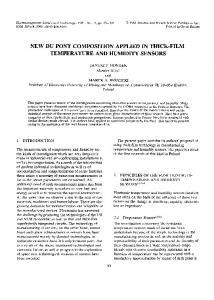
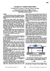
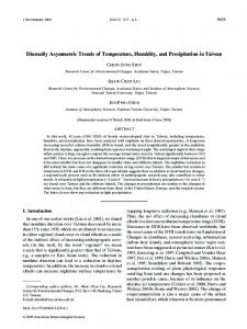
of Remote radiosonde temperature and humidity measurements can vary significantly for different4 sensor Sens. 2016, 8, 280 of 17 types [20]. To serve as a calibration database for remotely-sensed data, it is necessary that the selected with good good quality. quality.Among Amongradiosonde radiosonde selectedradiosonde radiosondemeasurements measurements have have self-consistency self-consistency with types, measurements fromfrom RS92RS92 radiosondes have been providetohomogeneous observations types, measurements radiosondes haveshown been toshown provide homogeneous in global locations arestudy used for in this for the biasprocess calibration in observations global locations [21] and, thus,[21] theyand, are thus, used they in this the study bias calibration of the process of the global tropospheric temperature and humidity retrievals. global tropospheric temperature and humidity retrievals. 2.2.2.2. Carbon Dioxide Carbon DioxideEffect Effect Observationsatat Mauna Mauna Loa riserise of CO in the decadesdecades [22]. Since Observations Loashow showsignificant significant of 2 CO theseveral past several [22]. 2 inpast HIRS observation began in 1978, the atmospheric CO2 concentration has increased from below 335 Since HIRS observation began in 1978, the atmospheric CO2 concentration has increased from below to to over 400400 ppmv. To examine the CO 2 effect, radiative transfer transfer model, RTTOV is used 335ppmv ppmv over ppmv. To examine the CO2 aeffect, a radiative model,[23], RTTOV [23], to simulate HIRS brightness temperatures in an increasing CO 2 environment. The use of a model is used to simulate HIRS brightness temperatures in an increasing CO2 environment. The use of facilitates the separation of CO2 effect any other changes. A diverse sample of global profiles a model facilitates the separation of COfrom 2 effect from any other changes. A diverse sample of global analyzed by the European Center for Medium-range Weather Forecasts (ECMWF) system [24] is profiles analyzed by the European Center for Medium-range Weather Forecasts (ECMWF) system [24] used to represent the atmospheric conditions. For the model simulations, the input profiles are kept is used to represent the atmospheric conditions. For the model simulations, the input profiles are unchanged except for the CO2 concentrations, and RTTOV is run for the CO2 concentrations of 330 kept unchanged except for the CO2 concentrations, and RTTOV is run for the CO2 concentrations of and 410 ppmv, respectively. The averaged brightness temperature of the global results for each HIRS 330 and 410 ppmv, respectively. The averaged brightness temperature of the global results for each channel is calculated. The differences of channel brightness temperatures between the two CO2 HIRS channel is calculated. The differences of channel brightness temperatures between the two CO2 concentration values are displayed in Figure 1. concentration values are displayed in Figure 1. Channel differences between CO2 amount of 410 and 330 ppmv

Tb(410) − Tb(330) (K)

1 0.5 0 −0.5 −1 −1.5 −2

1

2

3

4

5

6 7 Channel

8

9

10

11

12

Figure RTTOVmodel modelsimulation simulation of of brightness brightness temperature 1–12 Figure 1. 1.RTTOV temperaturedifferences differencesfor forHIRS HIRSchannels channels 1–12 2 amount of 410 and 330 ppmv. between CO between CO2 amount of 410 and 330 ppmv.

The weightingfunctions functionsofofHIRS HIRSCO CO2 absorption absorption channels ofof CO 2. With The weighting channelsvary varywith withthe theamount amount CO 2 2 . With the increase in CO2, the atmosphere becomes more opaque to the HIRS CO2 sounding channels, the increase in CO2 , the atmosphere becomes more opaque to the HIRS CO2 sounding channels, therefore the peaks of these channels’ weighting functions go up. As the mean temperature lapse therefore the peaks of these channels’ weighting functions go up. As the mean temperature lapse rate rate in the troposphere decreases with height and, vice versa, in the stratosphere, there is a negative in the troposphere decreases with height and, vice versa, in the stratosphere, there is a negative and and positive impact in the troposphere and stratosphere, respectively. For easy reference, the positive impact in the troposphere and stratosphere, respectively. For easy reference, the absorbents absorbents of HIRS longwave channels and the approximate broad layers where the channels sense of are HIRS longwave and the approximate layers wherewere the channels sense are listed listed in Tablechannels 1. The simulation shows that ifbroad CO2 concentration the only change in the in atmosphere, Table 1. Thewhen simulation shows that COppmv were only changefrom in the atmosphere, 2 concentration CO2 increases fromif330 to 410 ppmv, thethe measurements HIRS would when CO increases from 330 ppmv to 410 ppmv, the measurements from HIRS would appear 2 decrease in channels 4–7. The largest impact occurs in channels 5 and 6, with a value appear to as to decrease channels The largest impact occurs in channels 5 and 6, with a value as large ´2.0 large asin−2.0 K. The4–7. decreases of brightness temperatures for channels 4, and 7 are −1.6 and as −1.0 K, K. The decreases For of brightness temperatures for channels 4, and 7 are ´1.6 and ´1.0 K,from respectively. respectively. channels sensing the stratosphere (channels 1 and 2), the measurements HIRS Forobservation channels sensing stratosphere 1 and the measurements from HIRS observation would the appear larger in (channels an increased CO2), 2 environment. The increases in these two would appear in an CO2 environment. The increases in these twolower channels are 0.8 and channels arelarger 0.8 and 0.6 increased K, respectively. Channel 3 senses temperatures in the stratosphere the tropopause where the lapse rate is small and, thus,lower there stratosphere is not much effect the CO2 0.6near K, respectively. Channel 3 senses temperatures in the near from the tropopause change. on channels 8–12isbecause these are window ozone channel, where the There lapse are ratenoisimpacts small and, thus, there not much effect from thechannel, CO2 change. There are and water vapor channels. Figure 1 shows that there are large effects from CO 2 increase on several no impacts on channels 8–12 because these are window channel, ozone channel, and water vapor temperature sounding channels. If these effects are not considered in the temperature profile

Remote Sens. 2016, 8, 280

5 of 17

channels. Figure 1 shows that there are large effects from CO2 increase on several temperature sounding channels. If these effects are not considered in the temperature profile retrieval, it can lead to an underestimation of tropospheric temperatures and an overestimation of stratospheric temperatures in the HIRS measurements in an increasing CO2 environment. Table 1. Absorbents of HIRS longwave channels and the approximate broad layers where the channels sense. Channel

Absorption

Altitude (hPa)

1 2 3 4 5 6 7 8 9 10 11 12

CO2 CO2 CO2 CO2 CO2 CO2 CO2 (window) O3 Water vapor Water vapor Water vapor

5–100 20–150 30–300 80–500 300–800 400–1000 600–1000 Surface 10–100 700–1000 400–800 250–500

2.3. Retrieval The analysis above shows that it is a requirement for the retrieval algorithm to be able to account for CO2 effect on HIRS observations. This can be accomplished by the use of a radiative transfer model. As the RTTOV model is developed to simulate satellite sounder measurements with HIRS as one of the main sounders in the design, the model is chosen in the present study as a tool to build a retrieval training dataset. Selections of the ECMWF sampled profiles [24] provide the input database to RTTOV. The profile dataset was formed by carefully analyzing reanalysis data to extract a subset that has a global representation. Millions of global profiles from two years of the ECMWF analysis fields were divided into seven groups according to total precipitable water vapor contents at the interval of 0.5 kg¨ m´2 . About the same number of samples from each group was extracted, except for the group with the smallest total precipitable water vapor content, where twice as many profiles were extracted. Only the clear-sky profiles from the ECMWF sample profiles are used for the present study, which are comprised of 6891 profiles covering all latitudes and longitudes. The HIRS channel brightness temperatures for the reference satellite of the inter-calibrated dataset, Metop-A, are simulated by the radiative transfer model RTTOV. Tests are carried out with the use of RTTOV on the sensitivity of surface emissivity errors on retrievals. Results show that surface emissivity has a significant impact on the surface and near-surface temperatures. A variation of 0.2 in emissivity can have an impact of 1.1 ˝ C on the surface skin temperature and 0.7 ˝ C on surface air temperature. Therefore, surface emissivity is included as an input for the retrieval of surface and near-surface variables. The impact is reduced to less than 0.3 ˝ C at levels 850 hPa and up. The impact is small on specific humidity. With an emissivity variation of 0.2, the impact is 0.17 g/kg near the surface and smaller toward upper levels. Among the HIRS channels, the input to the upper air temperature retrievals consists of channels 2–12, and for the upper air specific humidity retrievals the input channels include the tropospheric channels 4–8 and 10–12. For the surface retrievals, only channels with sensitivity to the surface are used, which include channels 7, 8, and 10. Monthly mean values of CO2 observation from Mauna Loa are included in the input. The surface emissivity values are taken from the ISCCP dataset [7]. Outputs from the three neural networks are temperature profiles, including surface skin temperature, air temperature at the reference height of 2 m, and temperature at standard pressure levels from 1000 or the lowest pressure level above the surface to 50 hPa, and humidity profiles including specific

Remote Sens. 2016, 8, 280

6 of 17

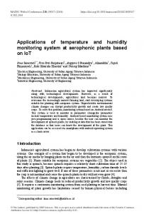
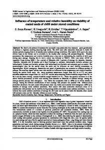
humidity at 2 m and at standard pressures from 1000 hPa or the lowest pressure level above the surface to 300Remote hPa.Sens. 2016, 8, 280 6 of 17 As atmospheric profiles over high surface elevations can differ significantly from those over low Asthe atmospheric profiles over high differaccording significantly from those over elevations, clear-sky training dataset is surface dividedelevations into threecan groups to the surface elevation low elevations, clear-sky training datasetusing is divided into three groups according the surface in terms of surfacethe pressure (Ps) calculated the hydrostatic equation. The to three groups are elevation in700 terms of 700 surface (Ps)hPa, calculated hydrostatic three defined as Ps < hPa, hPa pressure ď Ps < 850 and Psusing ě 850the hPa. Figure 2equation. shows a The global map of groups are defined as Ps < 700 hPa, 700 hPa ≤ Ps < 850 hPa, and Ps ≥ 850 hPa. Figure 2 shows a global where the groups are located. The vast majority of areas are in the group with Ps > 850 hPa. From each map of where the groups are located. The vast majority of areas are in the group with Ps > 850 hPa. surface elevation group, collocated data are randomly divided into three sub-groups at 60%, 20% and From each surface elevation group, collocated data are randomly divided into three sub-groups at 20%. 60%, The 60% is assigned to be the trainingtodataset. A testing dataset formed by one 20% sub-group and 20%. The 60% sub-group is assigned be the training dataset. A is testing dataset is 20% sub-group to use during iterations of neural network development. The remaining 20% is set aside formed by one 20% sub-group to use during iterations of neural network development. The for assessing the performance of for theassessing retrieval.the performance of the retrieval. remaining 20% is set aside

Figure 2. Surface elevation groups.The Thegrayscale grayscale assignments gray forfor Ps ≥Ps850 dark dark Figure 2. Surface elevation groups. assignmentsare arelight light gray ě hPa, 850 hPa, gray for 700 hPa ≤ Ps < 850 hPa, and black for Ps < 700 hPa. gray for 700 hPa ď Ps < 850 hPa, and black for Ps < 700 hPa.

A neural network approach is applied to connect temperature and humidity profiles with the

A neural network approach is applied toThe connect temperature humidity profiles with the HIRS longwave channel measurements. use of the neuraland network technique enables theHIRS longwave channel of measurements. use of the neuralthe network technique the establishment establishment the non-linear The relationship between retrieved variables enables and channel radiance retrievals with athe neural network scheme isand fast.channel Processing 35 yearsobservations. of HIRS of theobservations. non-linear Running relationship between retrieved variables radiance retrievals using a Linux computer platform that has a moderate specification takes about a week tousing Running retrievals with a neural network scheme is fast. Processing 35 years of HIRS retrievals complete, and processing in parallel reduces this even further. a Linux computer platform that has a moderate specification takes about a week to complete, and Different neural networks are built for the retrievals of the upper air temperature, upper air processing in parallel reduces this even further. specific humidity, and surface temperature and humidity. Neural networks have been used in past Different neural networks are built for the retrievals of the upper air temperature, upper air specific studies to retrieve atmospheric temperature and humidity along with other variables. For example, a humidity, and surface temperature and humidity. Neural networks haveatmospheric been used in past studies to three-layer backpropagation neural network was applied to derive temperature retrieve atmospheric temperature and humidity along with other variables. For example, a three-layer profiles from AMSU-A measurement [25]. The retrieved variables included surface air temperature, backpropagation network derive atmospheric temperatureheight, profiles temperatures atneural 26 pressure levelswas fromapplied 1000 to 10tohPa, and the tropopause temperature, and from pressure over both land ocean surfaces. Multi-layer backpropagation weretemperatures used to AMSU-A measurement [25].and The retrieved variables included surface airapproaches temperature, water vapor, cloud liquid water path, temperature, and emissivity over land at 26derive pressure levels from 1000 to 10 hPa, andsurface the tropopause temperature, height, andfrom pressure satellite microwave observations [26] and derive temperature, water vapor, and ozone profiles over both land and ocean surfaces. Multi-layer backpropagation approaches were used from to derive observations [27].water Three-layer feed-forward neural networks were also used retrieve waterIASI vapor, cloud liquid path, surface temperature, and emissivity over landtofrom satellite near-surface atmospheric variables over the ocean surfaces including SST, Ta, Qa, and wind speed microwave observations [26] and derive temperature, water vapor, and ozone profiles from IASI [28]. In the present study, three-layer backpropagation networks, with one input layer, one hidden observations [27]. Three-layer feed-forward neural networks were also used to retrieve near-surface layer, and one output layer, are constructed for the retrievals of temperature and humidity. atmospheric variablesinover the ocean surfaces including SST, in Ta, Qa, and wind speed [28]. As described the previous AMSU-A retrieval study [25], a backpropagation network, eachIn the present study, three-layer backpropagation networks, withWhen one input layer, one hidden layer, and layer is fully connected to the layers below and above. the network is given an input, the one output layer, are constructed forpropagates the retrievals of temperature andlayer humidity. updating of activation values forward from the input through the internal layer to the output layer. Each neuron in the output layer produces an output, which is compared to the

Remote Sens. 2016, 8, 280

7 of 17

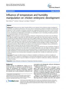
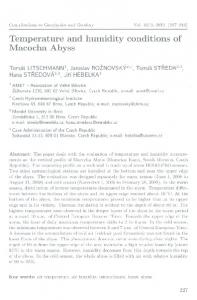
As described in the previous AMSU-A retrieval study [25], in a backpropagation network, each layer is fully connected to the layers below and above. When the network is given an input, the updating of activation values propagates forward from the input layer through the internal layer to Sens. 2016, 8, 280 neuron in the output layer produces an output, which is compared to the 7 of 17 theRemote output layer. Each target output defined in the training dataset. An error value is calculated for each neuron in the output layer. output defined in the training dataset. An error value is calculated for each neuron in the Thetarget network corrects its parameters to lessen the errors. The correction mechanism starts with the output layer. The network corrects its parameters to lessen the errors. The correction mechanism output neurons and propagates backward through the internal layer to the input layer. The iteration starts with the output neurons and propagates backward through the internal layer to the input continues until pre-set convergence criteria are met. layer. The iteration continues until pre-set convergence criteria are met. The converged neural network parameters are applied to the data that were set aside and were The converged neural network parameters are applied to the data that were set aside and were not used in the construction of the neural network to evaluate the network performance. The RMSEs not used in the construction of the neural network to evaluate the network performance. The RMSEs of temperature and specific the outputs outputsininthe thevalidation validation database of temperature and specifichumidity humidityare arecalculated calculated assuming assuming the database ˝ C for the temperature at the lowest as truth data. For temperature, the RMSEs are approximately 2.7 as truth data. For temperature, the RMSEs are approximately 2.7 °C for the temperature at the lowest ˝ in the mid-troposphere, and 1.5–2.6 ˝ C around the tropopause and standard pressure levels, 1.3–1.5 standard pressure levels, 1.3–1.5C°C in the mid-troposphere, and 1.5–2.6 °C around the tropopause in the For theFor specific humidity, the RMSE is 2.0 g/kg 1000athPa, steadily andlower in thestratosphere. lower stratosphere. the specific humidity, the RMSE is 2.0atg/kg 1000and hPa,it and it decreases to 1.1 g/kg at 700 hPa, and less than 0.4 g/kg above 500 hPa. The RMSEs for temperature and steadily decreases to 1.1 g/kg at 700 hPa, and less than 0.4 g/kg above 500 hPa. The RMSEs for humidity profiles athumidity standard profiles pressureatlevels calculated from data not usedfrom during network calibration temperature and standard pressure levels calculated data not used during arenetwork plotted in Figure 3. are These errorin estimates represent the uncertainty error structures from theerror model calibration plotted Figure 3. These error estimates represent the uncertainty structuresand from model simulation and the neural network scheme. simulation thethe neural network scheme.

Figure Usinga aset setofofdata datathat thatconsist consist of of simulated simulated HIRS HIRS channel byby Figure 3. 3. Using channel brightness brightnesstemperatures temperatures RTTOV with ECMWF profile input that are not used in the retrieval scheme development, retrieval RTTOV with ECMWF profile input that are not used in the retrieval scheme development, retrieval performances upper air profiles over different elevations (represented by pressures) surface performances for for upper air profiles over different surfacesurface elevations (represented by surface pressures) are examined. The RMSEs are shown in the figure for temperature (in °C, left panel) and are examined. The RMSEs are shown in the figure for temperature (in ˝ C, left panel) and specific specific humidity (in g/kg, right panel). humidity (in g/kg, right panel).

One of the error sources may come from channel observation noises. The NOAA Polar Orbiter One of the error mayKLM comeUser’s fromGuide channel noises. Polar Data User’s Guide [29]sources and NOAA [30] observation show that values of theThe noiseNOAA equivalent Orbiter Data User’s Guide [29] and NOAA KLM User’s Guide [30] show that values of differential radiance (NEΔN) for HIRS longwave channels are in the range ofthe 2·sr·cm−1) for 2·sr·cm−1channels noise equivalent differential radiance for3.00 HIRS longwave are 1.inChannel the range 0.10–0.65 mW/(m channels(NE∆N) 2–12, and mW/(m ) for channel 1 is of ´1 ) for channel 1. Channel 1 0.10–0.65 mW/(m ) for channels and 3.00 mW/(m ¨ sr¨ cm´1scheme ¨ sr¨ cm not used in the 2retrieval because2–12, of the concern on the 2high NEΔN. Using the developed is not used in the retrieval scheme of the concern onnoise the high NE∆N. Using the developed neural networks, a sensitivity testbecause is performed by adding to each of channels 2–12 in the training dataset, one channel at is a time, to examine how much it produces in in thethe retrieval neural networks, a sensitivity test performed by adding noise difference to each of channels 2–12 training results. Thechannel result for pressure level that corresponds to the mean weighting peak of an dataset, one at the a time, to examine how much difference it produces infunction the retrieval results. individual channel from an added noise value of 0.5 K is displayed in Tables 2 and 3. The channel The result for the pressure level that corresponds to the mean weighting function peak of an individual NEΔNfrom values are included in the tables provide in typical of The channel noises. Forvalues the channel an added noise value of 0.5 K isto displayed Tablesvalues 2 and 3. channel NE∆N 2 −1 sounding NEΔN values valuesofofchannel 0.10–0.65 mW/(m ·sr·cm ) approximately aretemperature included in the tables tochannels, provide typical noises. For the temperature sounding correspond to brightness temperature noises of 0.1–0.5 K. Different noise values are tested. A value 2 ´ 1 channels, NE∆N values of 0.10–0.65 mW/(m ¨ sr¨ cm ) approximately correspond to brightness of −0.5 K produces about the same impact as that from a value of 0.5 K, but with the opposite temperature noises of 0.1–0.5 K. Different noise values are tested. A value of ´0.5 K producessign. about Halving the noise value approximately halves the impact. the same impact as that from a value of 0.5 K, but with the opposite sign. Halving the noise value approximately halves the impact.

Remote Sens. 2016, 8, 280

8 of 17

Table 2. Sensitivity test of temperature sounding channel noises on the retrievals. The impact is based on adding 0.5 K noise to individual channel brightness temperatures. The levels shown are the approximate peaks of individual channels’ weighting functions. The NE∆N values (mW/(m2 ¨ sr¨ cm´1 )) are taken from NOAA KLM User’s Guide. Channel

Weighting Function Peak (hPa)

Impact on Retrieval (K)

NE∆N

2 3 4 5 6 7 8 9

100 200 300 500 700 850 surface 50

´1.646 ´2.039 2.669 2.258 1.589 1.235 0.827 ´0.212

0.67 0.50 0.31 0.21 0.24 0.20 0.10 0.15

Table 3. Similar to Table 2 for sensitivity tests of water vapor channel noise on the retrievals. Channel

Weighting Function Peak (hPa)

Impact on Retrieval (g/kg)

NE∆N

10 11 12

850 600 400

´0.364 ´0.376 ´0.004

0.15 0.20 0.20

2.4. Cloud Screening Retrieving atmospheric temperature and humidity profiles from an infrared instrument requires clear-sky conditions. When clouds are present, an infrared sounder, such as HIRS, can only sense to the top of clouds. The development of temperature and humidity profile retrievals is, therefore, based on clear-sky HIRS pixels. The clearing of cloudy pixels employs a two-tiered approach. The first cloud filtering is based on a simplified cloud detection procedure [31] as in ISCCP [32]. Cloudy pixels are first identified by comparisons of brightness temperature differences both spatially and temporally, among neighboring pixels in days before and after. Though the majority of clouds are cleared by this approach, a small portion of cloudy pixels having small spatial and temporal variations can be misclassified as clear pixels in the process. Often these are semi-permanent stratiform clouds. A second approach using cloud products derived from the Advanced Very High Resolution Radiometer (AVHRR) on board the same satellites, is added to further screen the clear-sky pixels identified in the first approach. The cloud products are part of the AVHRR Pathfinder Atmospheres-Extended (PATMOS-x) CDR dataset acquired from NOAA’s National Centers for Environmental Information [33]. PATMOS-x generates mapped products with a spatial resolution of 0.1 degrees on a global latitude-longitude grid. Two products, the cloud fraction and cloud probability, from the PATMOS-x dataset are chosen to screen the likelihood of cloud contamination in the HIRS pixels identified in the first step. An optimization scheme is used to find the optimal thresholds for cloud fraction and cloud probability to identify HIRS pixels that have high likelihood of being cloudy and, therefore, should not be used to derive clear-sky profiles. The HIRS temperature retrievals are compared to co-located RS92 observations in the lower atmosphere at 850 hPa. The optimization scheme finds the thresholds for cloud fraction and cloud probability that result in maximum correlation between HIRS retrievals and RS92 observations and minimum standard deviation of their differences, with the maximum amount of HIRS data retained. The optimal thresholds are found to be 0.5812 for cloud fraction and 0.9638 for cloud probability. The HIRS pixels having either higher values of cloud fraction or cloud probability as determined from PATMOS-x products are considered likely cloud-contaminated and should not be used, as is indicated with associated quality flags. Associated with each observation in the final dataset, a quality flag value is set indicating: (0) clear, (1) possibility of partially cloudiness, (2) likely cloudy, and (3) no cloud fraction/probability information available.

Remote Sens. 2016, 8, 280

9 of 17

2.5. Retrieval Calibration The aim of the retrieval algorithm development is to have outputs that are consistent with conventional global observations in terms of minimized systematic differences. Multiple factors may contribute to the systematic differences. The use of model simulations may have model-related biases, and a retrieval scheme may carry retrieval biases. In this study the upper air outputs from model-simulation-based neural networks are calibrated to radiosonde observations from RS92 and GPS RO profiles to achieve a systematically consistent dataset with the conventional measurements. For the upper air temperature and humidity retrievals in the troposphere, the calibration database is comprised of RS92 radiosonde observations. For the temperature outputs in the stratosphere, the retrievals are calibrated to GPS RO profiles. Pixels with cloud quality flags 0 and 1 (as defined above) were used to co-locate with RS92 and COSMIC2013 data for the calibration scheme development. The co-location criteria are within 0.1 latitude/longitude degree and 1 h at each pressure level. For each pressure level, and the northern and southern hemispheres separately, a multiple linear regression was performed. Additionally, for temperature, individual regressions were done for each 10 degree temperature bin; four bins of specific humidity values, each having approximately the same number of matchups, were created for each pressure level from the calibration dataset. Then, setting: ε “ TH IRS ´ Tind

(1)

where T H IRS is HIRS retrieval at a standard pressure level, and Tind is COSMIC2013 or RS92 we regress to find a, b, and c such that: ε “ a ` b ˚ TH IRS ` c ˚ L H IRS (2) where L H IRS is the latitude of the T H IRS observation. From here, the data was corrected as: TH IRS,new “ p1 ´ bq ˚ TH IRS ´ c ˚ L H IRS ´ a

(3)

An analogous method was used for specific humidity. To avoid artifacts along the equator which may arise from the hemisphere-specific regressions, smoothing was applied to all data located between ´10 and 10 degrees latitude. The associated latitude value was used as the linear interpolant for the smoothing. After bias calibrations were applied to the specific humidity data, a final quality control check was done to ensure that all specific humidity values were nonnegative and monotonically decreasing with increasing altitude. If a specific humidity value is found not monotonically decreasing with altitude, the value above is adjusted to the value below. No vertical adjustment is applied to temperature profiles. In many places, persistent temperature inversions are well captured in the retrievals. Temperature and specific humidity retrievals over southern high latitudes are not calibrated due to the very limited radiosonde measurements in the region for which no meaningful statistics can be generated. Over the Antarctic, more surface in situ long-term observations are required to establish a climate calibration benchmark. The left panels in Figures 4 and 5 show the remaining errors in terms of RMSEs of the retrievals globally and for different latitude bands after the calibration is applied. The standard deviation (STD) values for both HIRS retrievals (solid lines) and radiosonde or GPS RO observations (dashed lines) are included in the right panels to provide a context of variability at the standard pressure levels. There are about 3500 HIRS and radiosonde match-ups and about 4000 HIRS and GPS RO match-ups for pressure levels 850 hPa and above. The number of match-ups is less for 1000 hPa (about 1600), as the elevations of some areas are higher and thus there are no measurements available. The STD values of radiosondes and GPS RO profiles are consistently larger than those of HIRS retrievals. This indicates the difference between the footprint area measurement of HIRS and the point measurement from radiosondes or GPS RO, among other factors contributing to the differences. Globally, the RMSEs for the temperatures are in the range of 2–3 ˝ C at the lower tropospheric levels, 1.4–1.6 ˝ C at the mid-

Remote Remote Sens. Sens. 2016, 2016, 8, 8, 280 280

10 10 of of 17 17

Remote Sens. 2016, 8, 280

10 of 17

differences. Globally, the RMSEs for the temperatures are in the range of 2–3 °C at the lower tropospheric levels, 1.4–1.6 °C at the mid- and upper-tropospheric levels, and 2.1–2.3 °C at the ˝ Cin stratospheric levels. The levels, temperature RMSEs latitudes levels. are, generally, smaller than the and upper-tropospheric and 2.1–2.3 at the the low stratospheric The temperature RMSEs global RMSEs. The temperature RMSEs in the troposphere higher latitude bands as in the low latitudes are, generally, smaller than the global increase RMSEs. toward The temperature RMSEs in the there is larger variability of temperatures in midto high-latitudes. For specific humidity, the global troposphere increase toward higher latitude bands as there is larger variability of temperatures in RMSEs 2.4 g/kg at 1000 hPa, and steadily decrease 1.6 g/kg 700g/kg hPa,at 0.51000 g/kghPa, at 500 and mid- to are high-latitudes. For specific humidity, the globaltoRMSEs areat2.4 andhPa, steadily 0.05 g/kgtoat1.6 300 hPa.atThe band proportional the high decrease g/kg 700 largest hPa, 0.5RMSEs g/kg atare 500from hPa, the and low 0.05 latitude g/kg at 300 hPa. The largestto RMSEs are humidity values in the tropics. from the low latitude band proportional to the high humidity values in the tropics.

˝ C) compared Figure Figure 4. 4. HIRS HIRS derived temperature compared to 2011–2012 radiosonde (1000–400 hPa) and and GPS GPS Figure 4. HIRS derived derived temperature temperature (°C) ((°C) compared to to 2011–2012 2011–2012 radiosonde radiosonde (1000–400 (1000–400 hPa) hPa) and GPS RO (300–50 hPa) profiles for global and latitude bands for (a) RMSE and (b) STD (solid lines for HIRS RO (300–50 (300–50 hPa) hPa) profiles profiles for for global global and and latitude latitude bands bands for for (a) (a) RMSE RMSE and and (b) (b) STD STD (solid (solid lines lines for for HIRS HIRS RO and RO values). RO values). values). and dashed dashed lines lines for for radiosonde radiosonde or or GPS GPS RO

Figure 5. 5. HIRS HIRS derived specific humidity (g/kg) compared to 2011–2012 RS92 observations for derived specific humidity (g/kg) compared to RS92 for 5. HIRS derived specific humidity (g/kg) compared to 2011–2012 2011–2012 RS92 observations observations for global global global and latitude bands for (a)and RMSE and(solid (b) STD (solid linesand for dashed HIRS and dashed lines for and bands (a) (b) lines for lines for and latitude latitude bands for for (a) RMSE RMSE and (b) STD STD (solid lines for HIRS HIRS and dashed lines for radiosonde radiosonde radiosonde values). values). values).

Remote Sens. 2016, 8, 280 Remote Sens. 2016, 8, 280

11 of 17 11 of 17

The mean bias errors (MBEs) after the calibration procedure between the retrievals and 2011–2012 The mean bias (MBEs) after theincalibration the retrievals 2011– radiosonde and GPS ROerrors profiles are shown Figure 6. procedure The biasesbetween are defined as HIRSand values minus 2012 radiosonde and GPS RO profiles are shown in Figure 6. The biases are defined as HIRS values radiosonde or GPS RO values. Globally, the MBEs at all levels are zero for both temperature and minus radiosonde orshows GPS ROthat values. thehas MBEs at all levels are zero forof both temperature specific humidity. This the Globally, calibration accomplished the goal minimizing biases and specific humidity. This shows that the calibration has accomplished the goal of minimizing in a global mean. Very small biases remain in differentiated latitude bands. For temperature, the biases in a global mean. Very small biases remain in differentiated latitude bands. For temperature, biases are mostly less than ˘0.1 ˝ C for the mid-tropospheric to stratospheric levels. For the rest of the the biases are mostly less than ±0.1 °C for the˝ mid-tropospheric to stratospheric levels. For the rest of pressure levels the biases are less than ˘0.6 C. For the specific humidity, the tropical band has the the pressure levels the biases are less than ±0.6 °C. For the specific humidity, the tropical band has smallest biases with values less than g/kg, andand over thethe mid-latitude are less the smallest biases with values less˘0.04 than ±0.04 g/kg, over mid-latitudebands, bands, the the biases biases are than less ˘0.15 g/kg. Over high latitudes, the co-located data are noisier and have a smaller number than ±0.15 g/kg. Over high latitudes, the co-located data are noisier and have a smaller number of matches; thus, the resulting biases are larger. of matches; thus, the resulting biases are larger.

Figure 6. The MBE HIRS retrievals retrievals compared to 2011–2012 radiosonde observations for global and Figure 6. The MBE ofofHIRS compared to 2011–2012 radiosonde observations for global latitude bands (HIRS values minus radiosonde values) for (a) temperature (°C) and (b) specific ˝ and latitude bands (HIRS values minus radiosonde values) for (a) temperature ( C) and (b) specific humidity (g/kg). humidity (g/kg).

The calibration of the surface air temperature was performed separately using U.S. Climate

The calibration of(USCRN) the surface air temperature wasnetwork performed separately using Climate Reference Network observations. The USCRN consists of more than 200U.S. stations in theNetwork contiguous U.S. and observations. more than twenty Alaska and Hawaii. One important goal of USCRN Reference (USCRN) TheinUSCRN network consists of more than 200 stations in is to provide satellite and validation [34]. Each sitegoal includes triple is to the contiguous U.S.data andfor more than calibration twenty in Alaska and Hawaii. One USCRN important of USCRN redundancy for thecalibration primary and air validation temperature[34]. and precipitation soil provide data for satellite Each USCRN sitevariables includes and triplefor redundancy moisture/temperature. Instrumentation is regularly calibrated to National Institute for Standards for the primary air temperature and precipitation variables and for soil moisture/temperature. and Technology standards. HIRS-derived surface temperatures were co-located with a full year of Instrumentation is regularly calibrated to National Institute for Standards and Technology standards. USCRN observations in the development of a linear regression equation for calibrating the retrievals HIRS-derived surface temperatures were co-located with a full year of USCRN observations in the to USCRN observations [35]. development of a linear regression equation for calibrating the retrievals to USCRN observations [35]. 3. Evaluation and Discussion

3. Evaluation and Discussion

The results shown in Figures 4–6 are based on 2011–2012 data that were used in the

The results shown Figures 4–6 are based on 2011–2012 that were in the development development of the in calibration scheme. To examine whetherdata the scheme canused be applied to other of theyears calibration To examine whether the scheme canwith be applied toGPS other to yield similar to yieldscheme. similar results, comparisons of HIRS retrievals RS92 and ROyears profiles for two other years (2013–2014) are carried out,RS92 andand Figures 7 and 8 show comparison results of results, comparisons of HIRS retrievals with GPS RO profiles for two other years (2013–2014) temperatures and specific humidity at standard pressure levels, respectively. Globally, the are carried out, and Figures 7 and 8 show comparison results of temperatures and specific humidity temperature RMSEs rangerespectively. 2.2–3.8 °C forGlobally, the low-tropospheric levels (700–1000 hPa), 2.2–3.8 1.6–1.9 °C ˝ Cfor at standard pressure levels, the temperature RMSEs range for the mid-tropospheric levels (600–400 hPa), and 2.2–2.5 °C for upper tropospheric and stratospheric low-tropospheric levels (700–1000 hPa), 1.6–1.9 ˝ C for mid-tropospheric levels (600–400 hPa), and levels (300–50 hPa). The RMSEs are mostly smaller for tropics, ranging 2.0–2.9 °C for 2.2–2.5 ˝ C for upper tropospheric and stratospheric levels (300–50 hPa). The RMSEs are mostly smaller for tropics, ranging 2.0–2.9 ˝ C for low-tropospheric levels, 1.4–2.0 for mid-tropospheric levels, and 1.8–2.5 ˝ C for upper tropospheric and stratospheric levels. For specific humidity, the global RMSE is

8, 280 RemoteRemote Sens. Sens. 2016,2016, 8, 280 Remote Sens. 2016, 8, 280

12 of 17 12 of 17 12 of 17

low-tropospheric levels, 1.4–2.0 for mid-tropospheric levels, and 1.8–2.5 °C for upper tropospheric low-tropospheric levels, 1.4–2.0 for mid-tropospheric °Cg/kg for upper tropospheric and stratospheric levels. For specific humidity, the levels, global RMSE is g/kg 2.4 at 1000 hPa, 0.06 and g/kg 2.4 g/kg at 1000 hPa, and decreases steadily to 1.6 g/kg at 700and hPa,1.8–2.5 0.5 at 500 hPa, and and Forat specific the hPa, global is 2.4 g/kg atas1000 hPa, and steadily tolevels. 1.6 g/kg 700 hPa, 0.5 g/kg at 500 andRMSE 0.06 g/kg at 300 hPa the humidity at 300decreases hPastratospheric as the humidity decreases withhumidity, height. decreases with to 1.6 g/kg at 700 hPa, 0.5 g/kg at 500 hPa, and 0.06 g/kg at 300 hPa as the humidity decreases height. The right steadily panels of Figures 7 and 8 show the biases of temperature and specific humidity profiles decreases with panels height. of Figures 7 and 8 show the biases of temperature and specific humidity The right compared to 2013–2014 radiosonde and GPS RO measurements. For temperature, except at 1000 hPa Thecompared right panels of Figures 7 and 8 show the RO biases of temperature and specific humidity profiles to 2013–2014 radiosonde and GPS measurements. For temperature, except at that has a bias of ´1 ˝ C, 2013–2014 the globalradiosonde mean biases are all within ˘0.3 ˝ C For for temperature, other levels.except For specific profiles GPS RO are measurements. at 1000 hPacompared that has atobias of −1 °C, the global and mean biases all within ±0.3 °C for other levels. For humidity, the global bias is°C, ´0.6 g/kg atmean 1000at hPa, at ±0.3 850 hPa, at 700 1000 hPa that hasmean a bias of −1 the global biases are within °ChPa, for0.04 other levels. For hPa, specific humidity, the global mean bias is −0.6 g/kg 1000´0.2 hPa,allg/kg −0.2 g/kg at 850 0.04g/kg g/kg at 700 and within 0.01 g/kg for the levels above. specific humidity, theg/kg global mean biasabove. is −0.6 g/kg at 1000 hPa, −0.2 g/kg at 850 hPa, 0.04 g/kg at 700 hPa, and within 0.01 for the levels hPa, and within 0.01 g/kg for the levels above.

Figure 7. HIRS derived temperature (°C) to 2013–2014 (in which data are not used for bias Figure 7. HIRS derived temperature (˝ C)compared compared to 2013–2014 (in which data are not used for Figure 7. HIRS derived temperature (°C) compared to 2013–2014 which data are hPa) not used for bias calibration scheme development) radiosonde (1000–400 hPa) and(in GPS RO (300–50 profiles for bias calibration scheme development) radiosonde (1000–400 hPa) and GPS RO (300–50 hPa) profiles calibration scheme development) radiosonde (1000–400 hPa) values and GPS RO (300–50 hPa)or profiles for global and latitude bands for (a) RMSE and (b) MBE (HIRS minus radiosonde GPS RO for global and latitude bands for (a) RMSE and (b) MBE (HIRS values minus radiosonde or GPS global and latitude bands for (a) RMSE and (b) MBE (HIRS values minus radiosonde or GPS RO values). RO values). values).

Figure 8. HIRS derived specific humidity (g/kg) compared to 2013–2014 radiosonde observations for Figure 8. HIRS derived specific humidity (g/kg) compared toto2013–2014 observations for for global and latitude bands for (a) RMSE and (b) MBE (HIRS values minus radiosonde radiosonde values). Figure 8. HIRS derived specific humidity (g/kg) compared 2013–2014 radiosonde observations global and latitude bands for (a) RMSE and (b) MBE (HIRS values minus radiosonde values).

global and latitude bands for (a) RMSE and (b) MBE (HIRS values minus radiosonde values). The RMSEs and MBEs shown above are based on retrievals from HIRS observation only. The RMSEs and MBEsand shown above are based on retrievals HIRS observation only. Operationally, temperature humidity profiles are often retrieved from from multiple instruments in The RMSEs and MBEs shown above are based on retrievals from HIRS observation Operationally, temperature and humidity profiles are often retrieved from multiple instruments in only. the TIROS Operational Vertical Sounder (TOVS) or ATOVS suite. The inclusion of multiple sounders thethe TIROS Operational Vertical SounderRMSEs. (TOVS) or ATOVS suite. The inclusion ofmultiple multiple sounders in retrievals is expected to reduce Using theoften TOVS instruments, which include HIRS, Operationally, temperature and humidity profiles are retrieved from instruments in theand retrievals is expected tohad reduce RMSEs. theRMSEs TOVS instruments, which include HIRS, SSU, the 3I method temperature retrieval of 1.5–2.25 K for the clear-sky case in theMSU, TIROS Operational Vertical Sounder (TOVS)Using or ATOVS suite. The inclusion of multiple sounders MSU, and SSU, the 3I method had3Itemperature retrieval ofinstruments, 1.5–2.25 K that for which the caseHIRS, A study on assessment the method the European Arctic showed theclear-sky temperature in the[3]. retrievals is expected toofreduce RMSEs.inUsing theRMSEs TOVS include [3]. A study onmean assessment of the 3I±1.5 method in the European Arctic showed that the temperature retrievals had biases within K [36]. For the IAPP method, the temperature retrieval MSU, and SSU, the 3I method had temperature retrieval RMSEs of 1.5–2.25 K for the clear-sky case [3]. retrievals had on mean biases ±1.5 K For the IAPP method, profiles the temperature RMSEs based HIRS andwithin AMSU-A for[36]. atmospheric temperature at 1-km retrieval vertical A study on assessment of the 3I method in the European Arctic showed that the temperature retrievals RMSEs based on HIRS and AMSU-A for atmospheric temperature profiles at 1-km vertical

had mean biases within ˘1.5 K [36]. For the IAPP method, the temperature retrieval RMSEs based on HIRS and AMSU-A for atmospheric temperature profiles at 1-km vertical resolution are 2.5 K for 1000–850 hPa, and about 1.3–2.0 K for layers in 500–70 hPa [4]. For the NOAA operational sounding products which uses HIRS, AMSU-A, and AMSU-B, the temperature mean biases are mostly within

Remote Sens. 2016, 8, 280 Remote Sens. 2016, 8, 280

13 of 17 13 of 17

resolution are 2.5 K for 1000–850 hPa, and about 1.3–2.0 K for layers in 500–70 hPa [4]. For the NOAA operational sounding products which uses HIRS, AMSU-A, and AMSU-B, the temperature mean ˘0.5 K for regionwithin 60˝ N to 60˝KS for [6]. The recent soundersfrom oftentimes biases arethe mostly ±0.5 the retrievals region 60°from N to 60° hyperspectral S [6]. The retrievals recent show reduced retrieval errors when compared to high-quality sondes [27,37]. Though the inclusion hyperspectral sounders oftentimes show reduced retrieval errors when compared to high-quality of additional sounding retrievalssounding may have smaller retrieval errors, none the sondes [27,37]. Though instruments the inclusioninofthe additional instruments in the retrievals mayofhave sounding instruments except HIRS has more than 37 years of observation time. The use of different smaller retrieval errors, none of the sounding instruments except HIRS has more than 37 years of sounding instruments a long-term timesounding series mayinstruments introduce significant discontinuity and thus observation time. Theinuse of different in a long-term time series may render the retrievals for climate applications. introduce significantunsuitable discontinuity and thus render the retrievals unsuitable for climate applications. When pixel retrieval is compared to a radiosonde observation, there arethere inherent Whena aHIRS HIRS pixel retrieval is compared to a radiosonde observation, are random inherent differences that are unrelated to retrieval errors. errors. For example, there there are differences between the random differences that are unrelated to retrieval For example, are differences between areal measurement of aofHIRS footprint andand thethe point measurement of of a radiosonde. the areal measurement a HIRS footprint point measurement a radiosonde.There There are are sampling differences when the observations are not made at exact same times. There is inhomogeneity sampling differences when the observations are not made at exact same times. There is among individual radiosonde measurements. The radiosondes used for comparison this study inhomogeneity among individual radiosonde measurements. The radiosondes used forincomparison are operational measurements that may contain launch-dependent biases. All of these factors can in this study are operational measurements that may contain launch-dependent biases. All of these contribute to the differences in the comparison analysis. To show the bias patterns between HIRS factors can contribute to the differences in the comparison analysis. To show the bias patterns retrievals and radiosonde observations, Figure 9 displaysFigure an example of thean bias histograms taken between HIRS retrievals and radiosonde observations, 9 displays example of the bias at 850 hPa for temperature (left panel) and specific humidity (right panel). There is a peak near theis histograms taken at 850 hPa for temperature (left panel) and specific humidity (right panel). There zero biasnear line,the andzero the bias majority observations is of distributed around the zero bias line. The patterns a peak line, of and the majority observations is distributed around the zero bias for other are for similar a peak near thewith zeroabias thin bothand sides. theatHIRS line. Thelevels patterns otherwith levels are similar peakand near thetails zeroatbias thinFor tails both retrievals this study, the intended is to the derive monthly for climate monitoring. With the sides. Forinthe HIRS retrievals in thisuse study, intended usemeans is to derive monthly means for climate bias patterns With similar those in Figure 9, the tails ofinthe biases are tails expected be smoothed out in monitoring. thetobias patterns similar to those Figure 9, the of thetobiases are expected to monthly means that can lead to significantly-reduced RMSEs in monthly means. be smoothed out in monthly means that can lead to significantly-reduced RMSEs in monthly means.

Figure9.9. Histograms Histograms of of the the biases biases(˝(°C) between HIRS HIRS retrievals retrievals and andradiosonde radiosondeobservations observations for for Figure C) between temperature temperature(a) (a)and andhumidity humidity(b) (b)atat850 850hPa. hPa.

HIRSderived derivedsurface surfaceair airtemperatures temperatureswere wereevaluated evaluatedusing usingUSCRN USCRNobservations observations[35]. [35].For Forthe the HIRS years that were not used in developing the calibration scheme, the mean biases of HIRS retrievals for years that were not used in developing the calibration scheme, the mean biases of HIRS retrievals for eachyear yearare aremostly mostlyin inthe therange rangeofof0.5–1.0 0.5–1.0˝°C, andthe theRMSEs RMSEsare are~1.6 ~1.6˝°C. Resultsfor forindividual individual each C, and C. Results stations have consistent biases within ±1.5 °C and RMSEs are less than 2 °C for most locations. HIRS ˝ ˝ stations have consistent biases within ˘1.5 C and RMSEs are less than 2 C for most locations. surface air temperatures werewere alsoalso compared to to thethe Surface Arctic Ocean Ocean HIRS surface air temperatures compared SurfaceHeat HeatBudget Budgetof of the the Arctic (SHEBA) observations. The SHEBA project was an interdisciplinary effort with a year-long field (SHEBA) observations. The SHEBA project was an interdisciplinary effort with a year-long field experiment in the Beaufort and Chukchi Seas. It produced a collection of atmospheric, experiment in the Beaufort and Chukchi Seas. It produced a collection of atmospheric, oceanographic, oceanographic, cryospheric taken measurements taken on a Canadian icebreaker frozen the arctic and cryosphericand measurements on a Canadian icebreaker frozen in the arctic iceinpack [38].

Remote Sens. 2016, 8, 280

14 of 17

For measurements co-located within 30 km and 30 min, the RMSE of clear-sky HIRS surface Remote Sens. 2016, 8, 280 14 of 17 air temperature retrievals over the Arctic Sea was found in the order of 1 ˝ C [39]. ice [38]. For measurements co-located within 30 HIRS km and 30 min, RMSE ofatclear-sky HIRS Thepack retrievals from this study apply to individual pixels. Thethe retrievals pixel observation surface air temperature retrievals over the Arctic Sea was found in the order of 1 °C [39]. times should not be directly used in a time series to infer climate variabilities without addressing Theeffect. retrievals apply individual pixels. The retrievals at sampling. pixel the diurnal HIRSfrom datathis fromstudy one or two to satellites mayHIRS not have a sufficient diurnal observation times should not be directly used in a time series to infer climate variabilities without However, there was an overlapping of four satellites (from NOAA-14, -15, -16, and -17) that lasted addressing the diurnal effect. HIRS data from one or two satellites may not have a sufficient diurnal several years. The twice-a-day observations from each satellite and the drifting of individual satellites’ sampling. However, there was an overlapping of four satellites (from NOAA-14, -15, -16, and -17) orbits during that period provided a good diurnal sampling. A diurnal variation model can be built that lasted several years. The twice-a-day observations from each satellite and the drifting of based on these satellites’ several years data, such as the one developed the ISCCP [7] and analysis individual orbitsofduring that period provided a goodindiurnal sampling. A the diurnal discussed in a study of HIRS channel diurnal cycles [40]. With a diurnal model in place, the variation model can be built based on these several years of data, such as the one developed in theHIRS retrievals further processed to daily monthly datasets usedcycles for its[40]. intended ISCCPcan [7]be and the analysis discussed in aand study of HIRS channeland diurnal With aapplications, diurnal in place, the HIRSlarge-scale retrievals can be further background processed to daily and monthly datasets and used i.e., tomodel provide a long-term, atmospheric for relevant climate product generation its intended applications, to provide and for climate monitoring on a i.e., monthly basis.a long-term, large-scale atmospheric background for relevant climate product andoverview for climateofmonitoring on a monthly In summary, Figure 10generation provides an the development workbasis. presented in Sections 2 In summary, Figure 10 provides an overview of the development work presented in Sections 2 and 3 of this study. In the figure new developments in this study are in the blue font, and related and 3 of this study. In the figure new developments in this study are in the blue font, and related developments outside of the study are in the green font. The algorithm development starts with developments outside of the study are in the green font. The algorithm development starts with neural network designs together with a test of CO2 effect. Cloud clearing is improved by additional neural network designs together with a test of CO2 effect. Cloud clearing is improved by additional information from AVHRR cloud products. Conventional observations are used for bias calibration. information from AVHRR cloud products. Conventional observations are used for bias calibration. The retrieved profiles areare evaluated bybyobservations usedin inthe theretrieval retrieval scheme development. The retrieved profiles evaluated observations not not used scheme development.

Figure 10. Overview of algorithm development. New developments in this study are listed in blue,

Figure 10. Overview of algorithm development. New developments in this study are listed in blue, and related developments outside of the study are in green. and related developments outside of the study are in green.

Remote Sens. 2016, 8, 280

15 of 17

4. Conclusions This article describes the retrieval algorithm development aspect of the project, towards developing a CDR of temperature and humidity profiles from HIRS clear-sky measurements. The development combines a neural network technique with the modeling of long-term CO2 effect and a calibration scheme based on conventional observations. During the last several decades of HIRS measurements, the atmospheric CO2 increased from 335 ppm to over 400 ppm. The increased amount of CO2 resulted mean negative impacts of ´1 K to ´2 K for the tropospheric channels and positive impacts of above 0.5 K for stratospheric channels 1 and 2. Such a long-term effect is accounted for in the retrieval algorithm for processing more than 36 years of HIRS observations. Using data from HIRS longwave channels as well as input of CO2 and emissivity values with the aid of a radiative transfer model, neural networks are built to derive temperature and specific humidity at standard pressure levels and near the surface. A two-tiered approach is applied to screen HIRS pixels to identify clear-sky pixels to reduce cloud contamination. Radiosonde observations and GPS RO profiles are incorporated to calibrate the upper air retrievals to achieve consistency of retrievals with these observations in the troposphere and in the stratosphere. The development of the calibration scheme accomplishes the goal of unbiased results, globally. To evaluate the retrieval algorithm, the procedure is applied to two years of HIRS observations that are not used in the algorithm development, and the retrievals are compared with radiosonde observations and GPS RO derived profiles. Except for the lowest level which exhibits larger variability, the global mean bias errors are small and within ˘0.3 ˝ C for temperature and within ˘0.2 g/kg for specific humidity. The focus of this article is on the algorithm development of the upper air temperature and specific humidity profile retrievals from HIRS as one part of a CDR dataset development project. Other parts of the project include inter-satellite calibration, validation of retrievals from all satellites using independent high-quality global coverage datasets, and the evaluation of surface temperature and humidity retrievals. The integration of all these parts constitutes an effort to build a homogenized long-term atmospheric temperature and humidity dataset based on HIRS observations since 1978 for climate studies. Acknowledgments: The AVHRR Clouds Properties—PATMOS-x CDR used in this study was acquired from NOAA’s CDR Program (http://www.ncdc.noaa.gov/cdr). This CDR was originally developed by Andy Heidinger and colleagues. Jessica Matthews was supported by NOAA through the Cooperative Institute for Climate and Satellites—North Carolina under Cooperative Agreement NA14NES432003. The authors thank Darren Jackson for providing HIRS limb-correction codes and codes for the first round of cloud-screening in this study, and thank Ken Knapp and three anonymous reviewers for constructive comments. Author Contributions: The research is designed by L.S., J.M., and J.B., J.M., L.S., Q.Y., and S.P.H. performed code development, data processing, and data analyses. L.S. and J.M. wrote the paper. All of the authors contributed to the paper through their review, editing and comments. Conflicts of Interest: The authors declare no conflict of interest.

References 1. 2. 3.

4.

Shi, L.; Bates, J.J.; Li, X.; Uppala, S.M.; Kelly, G. Extending the satellite sounding archive back in time: The vertical temperature profile radiometer data. J. Appl. Remote Sens. 2008, 2. [CrossRef] Susskind, J.; Rosenfield, J.; Reuter, D.; Chahine, M.T. Remote sensing of weather and climate parameters from HIRS2/MSU on TIROS-N. J. Geophys. Res. Atmos. 1984, 89, 4677–4697. [CrossRef] Chedin, A.; Scott, N.A.; Wahiche, C.; Moulinier, P. The improved initialization inversion method: A high resolution physical method for temperature retrievals from satellites of the TIROS-N series. J. Clim. Appl. Meteorol. 1985, 24, 128–143. [CrossRef] Li, J.; Wolf, W.W.; Menzel, W.P.; Zhang, W.J.; Huang, H.L.; Achtor, T.H. Global soundings of the atmosphere from ATOVS measurements: The algorithm and validation. J. Appl. Meteorol. 2000, 39, 1248–1268. [CrossRef]

Remote Sens. 2016, 8, 280

5. 6. 7. 8. 9. 10. 11. 12.

13. 14. 15. 16.

17.

18.

19.

20.

21. 22. 23. 24. 25. 26.

16 of 17

Fleming, H.E.; Crosby, D.S.; Neuendorffer, A.C. Correction of satellite temperature retrieval errors due to errors in atmospheric transmittances. J. Clim. Appl. Meteorol. 1986, 25, 869–882. [CrossRef] Reale, A.; Tilley, F.; Ferguson, M.; Allegrino, A. NOAA operational sounding products for advanced TOVS. Int. J. Remote Sens. 2008, 29, 4615–4651. [CrossRef] Rossow, W.B.; Dueñas, E.N. The international satellite cloud climatology project (ISCCP) web site: An online resource for research. Bull. Am. Meteorol. Soc. 2004, 85, 167–172. [CrossRef] Rossow, W. Clouds in weather and climate: The international satellite cloud climatology project at 30: What do we know and what do we still need to know? Bull. Am. Meteorol. Soc. 2014, 95, 441–443. [CrossRef] Chung, E.-S.; Soden, B.J. Radiative signature of increasing atmospheric carbon dioxide in hirs satellite observations. Geophys. Res. Lett. 2010, 37, L07707. [CrossRef] Chung, E.S.; Soden, B.J. Investigating the influence of carbon dioxide and the stratosphere on the long-term tropospheric temperature monitoring from HIRS. J. Appl. Meteorol. Clim. 2010, 49, 1927–1937. [CrossRef] Jackson, D.L.; Wylie, D.P.; Bates, J.J. The HIRS pathfinder radiance data set (1979–2001). In Proceedings of the 12th Conference on Satellite Meteorology and Oceanography, Long Beach, CA, USA, 10–13 February 2003. Cao, C.; Weinreb, M.; Xu, H. Predicting simultaneous nadir overpasses among polar-orbiting meteorological satellites for the intersatellite calibration of radiometers. J. Atmos. Ocean. Technol. 2004, 21, 537–542. [CrossRef] Cao, C.; Jarva, K.; Ciren, P. An improved algorithm for the operational calibration of the high-resolution infrared radiation sounder. J. Atmos. Ocean. Technol. 2007, 24, 169–181. [CrossRef] Shi, L.; Bates, J.J.; Cao, C. Scene radiance-dependent intersatellite biases of hirs longwave channels. J. Atmos. Ocean. Technol. 2008, 25, 2219–2229. [CrossRef] Shi, L. Intersatellite differences of HIRS longwave channels between NOAA-14 and NOAA-15 and between NOAA-17 and METOP-A. IEEE Trans. Geosci. Remote 2013, 51, 1414–1424. [CrossRef] Ho, S.P.; Goldberg, M.; Kuo, Y.H.; Zou, C.Z.; Schreiner, W. Calibration of temperature in the lower stratosphere from microwave measurements using cosmic radio occultation data: Preliminary results. Terr. Atmos. Ocean. Sci. 2009, 20, 87–100. [CrossRef] Ho, S.P.; Hunt, D.; Steiner, A.K.; Mannucci, A.J.; Kirchengast, G.; Gleisner, H.; Heise, S.; von Engeln, A.; Marquardt, C.; Sokolovskiy, S.; et al. Reproducibility of GPS radio occultation data for climate monitoring: Profile-to-profile inter-comparison of champ climate records 2002 to 2008 from six data centers. J. Geophys. Res. Atmos. 2012, 117. [CrossRef] Ho, S.P.; Kirchengast, G.; Leroy, S.; Wickert, J.; Mannucci, A.J.; Steiner, A.; Hunt, D.; Schreiner, W.; Sokolovskiy, S.; Ao, C.; et al. Estimating the uncertainty of using GPS radio occultation data for climate monitoring: Intercomparison of champ refractivity climate records from 2002 to 2006 from different data centers. J. Geophys. Res. Atmos. 2009, 114. [CrossRef] Ho, S.P.; Yue, X.; Zeng, Z.; Ao, C.O.; Huang, C.Y.; Kursinski, E.R.; Kuo, Y.H. Applications of COSMIC radio occultation data from the troposphere to ionosphere and potential impacts of COSMIC-2 data. Bull. Am. Meteorol. Soc. 2014, 95, ES18–ES22. [CrossRef] He, W.Y.; Ho, S.P.; Chen, H.B.; Zhou, X.J.; Hunt, D.; Kuo, Y.H. Assessment of radiosonde temperature measurements in the upper troposphere and lower stratosphere using cosmic radio occultation data. Geophys. Res. Lett. 2009, 36. [CrossRef] Ho, S.P.; Kuo, Y.H.; Schreiner, W.; Zhou, X. Using SI-traceable global positioning system radio occultation measurements for climate monitoring. Bull. Am. Meteorol. Soc. 2010, 91, S36–S37. Keeling, C.D.; Whorf, T.P.; Wahlen, M.; Vanderplicht, J. Interannual extremes in the rate of rise of atmospheric carbon-dioxide since 1980. Nature 1995, 375, 666–670. [CrossRef] Saunders, R.; Matricardi, M.; Brunel, P. An improved fast radiative transfer model for assimilation of satellite radiance observations. Q. J. R. Meteorol. Soc. 1999, 125, 1407–1425. [CrossRef] Chevallier, F. Sampled Databases of 60-Level Atmospheric Profiles from the ECMWF Analyses; NWPSAF-EC-TR-004; EUMETSAT: Darmstadt, Germany, 2001. Shi, L. Retrieval of atmospheric temperature profiles from AMSU-A measurement using a neural network approach. J. Atmos. Ocean. Technol. 2001, 18, 340–347. [CrossRef] Aires, F.; Prigent, C.; Rossow, W.B.; Rothstein, M. A new neural network approach including first guess for retrieval of atmospheric water vapor, cloud liquid water path, surface temperature, and emissivities over land from satellite microwave observations. J. Geophys. Res. Atmos. 2001, 106, 14887–14907. [CrossRef]

Remote Sens. 2016, 8, 280

27.

28.

29. 30. 31.

32. 33. 34.

35. 36.

37.

38.

39. 40.

17 of 17

Aires, F.; Rossow, W.B.; Scott, N.A.; Chédin, A. Remote sensing from the infrared atmospheric sounding interferometer instrument 2. Simultaneous retrieval of temperature, water vapor, and ozone atmospheric profiles. J. Geophys. Res. Atmos. 2002, 107, 4620. [CrossRef] Roberts, J.B.; Clayson, C.A.; Robertson, F.R.; Jackson, D.L. Predicting near-surface atmospheric variables from special sensor microwave/imager using neural networks with a first-guess approach. J. Geophys. Res. 2010, 115, D19113. [CrossRef] Kidwell, K.B. NOAA Polar Orbiter Data User’s Guide, 1998. Available online: http://www.ncdc.noaa.gov/ oa/pod-guide/ncdc/docs/podug/index.htm (accessed on 23 March 2016). Robel, J. NOAA KLM User’s Guide, 2009. Available online: http://www.ncdc.noaa.gov/oa/pod-guide/ ncdc/docs/klm/index.htm (accessed on 23 March 2016). Jackson, D.; Bates, J. A 20-yr TOVS radiance Pathfinder data set for climate analysis. In Proceedings of the 10th Conference on Satellite Meteorology and Oceanography, 80th AMS Annual Meeting, Long Beach, CA, USA, 9–14 January 2000. Rossow, W.B.; Garder, L.C. Cloud detection using satellite measurements of infrared and visible radiances for ISCCP. J. Clim. 1993, 6, 2341–2369. [CrossRef] Heidinger, A.K.; Foster, M.J.; Walther, A.; Zhao, X.P. The Pathfinder atmospheres-extended AVHRR climate dataset. Bull. Am. Meteorol. Soc. 2014, 95, 909. [CrossRef] Diamond, H.J.; Karl, T.R.; Palecki, M.A.; Baker, C.B.; Bell, J.E.; Leeper, R.D.; Easterling, D.R.; Lawrimore, J.H.; Meyers, T.P.; Helfert, M.R.; et al. U.S. Climate reference network after one decade of operations status and assessment. Bull. Am. Meteorol. Soc. 2013, 94, 485–498. [CrossRef] Stegall, S.T.; Shi, L. An assessment of HIRS surface air temperature with USCRN data. Remote Sens. 2016, submitted. Claud, C.; Scott, N.A.; Chedin, A.; Gascard, J.C. Assessment of the accuracy of atmospheric-temperature profiles retrieved from TOVS observations by the 3I-method in the European Arctic—Application for mesoscale weather analysis. J. Geophys. Res. Atmos. 1991, 96, 2875–2887. [CrossRef] Boylan, P.; Wang, J.H.; Cohn, S.A.; Fetzer, E.; Maddy, E.S.; Wong, S. Validation of AIRS version 6 temperature profiles and surface-based inversions over Antarctica using Concordiasi dropsonde data. J. Geophys. Res. Atmos. 2015, 120, 992–1007. [CrossRef] Uttal, T.; Curry, J.A.; McPhee, M.G.; Perovich, D.K.; Moritz, R.E.; Maslanik, J.A.; Guest, P.S.; Stern, H.L.; Moore, J.A.; Turenne, R.; et al. Surface heat budget of the Arctic Ocean. Bull. Am. Meteorol. Soc. 2002, 83, 255–275. [CrossRef] Peng, G.; Shi, L.; Stegall, S.T.; Matthews, J.L.; Fairall, C.W. An evaluation of HIRS near-surface air temperature product in the Arctic with SHEBA data. J. Atmos. Ocean. Techol. 2016, 33, 453–460. [CrossRef] Lindfors, A.V.; Mackenzie, I.A.; Tett, S.F.B.; Shi, L. Climatological diurnal cycles in clear-sky brightness temperatures from the high-resolution infrared radiation sounder (HIRS). J. Atmos. Ocean. Techol. 2011, 28, 1199–1205. [CrossRef] © 2016 by the authors; licensee MDPI, Basel, Switzerland. This article is an open access article distributed under the terms and conditions of the Creative Commons by Attribution (CC-BY) license (http://creativecommons.org/licenses/by/4.0/).