we will consider some basic aspects of graph theoretic algorithms such as, ..... is easy to work on all edges in a list consecutively, and to insert or remove edges.
Chapter 2
Algorithms and Complexity
If to do were as easy as to know what were good to do. . . William Shakespeare
In Theorem 1.3.1 we gave a characterization for Eulerian graphs: a graph G is Eulerian if and only if each vertex of G has even degree. This condition is easy to verify for any given graph. But how can we really find an Euler tour in an Eulerian graph? The proof of Theorem 1.3.1 not only guarantees that such a tour exists, but actually contains a hint how to construct such a tour. We want to convert this hint into a general method for constructing an Euler tour in any given Eulerian graph; in short, into an algorithm. In this book we generally look at problems from the algorithmic point of view: we want more than just theorems about existence or structure. As L¨ uneburg once said [Lue82], it is important in the end that we can compute the objects we are working with. However, we will not go as far as giving concrete programs, but describe our algorithms in a less formal way. Our main goal is to give an overview of the basic methods used in a very large area of mathematics; we can achieve this (without exceeding the limits of this book) only by omitting the details of programming techniques. Readers interested in concrete programs are referred to [SysDK83] and [NijWi78], where programs in PASCAL and FORTRAN, respectively, can be found. Although many algorithms will occur throughout this book, we will not try to give a formal definition of the concept of algorithms. Such a definition belongs to both mathematical logic and theoretical computer science and is given, for instance, in automata theory or in complexity theory; we refer the reader to [HopUl79] and [GarJo79]. For a general treatment, we also recommend the books [AhoHU74, AhoHU83] and, in particular, [CorLRS09], one of the standard text books on algorithms. In this chapter, we will try to show in an intuitive way what an algorithm is and to develop a way to measure the quality of algorithms. In particular, we will consider some basic aspects of graph theoretic algorithms such as, for example, the problem of how to represent a graph. Moreover, we need a way to formulate the algorithms we deal with. We shall illustrate and study these concepts quite thoroughly using two specific examples, namely Euler D. Jungnickel, Graphs, Networks and Algorithms, Algorithms and Computation in Mathematics 5, DOI 10.1007/978-3-642-32278-5 2, © Springer-Verlag Berlin Heidelberg 2013
35
36
2
Algorithms and Complexity
tours and acyclic digraphs. At the end of the chapter we introduce a class of problems (the so-called NP-complete problems) which plays a central role in complexity theory; we will meet this type of problem over and over again in this book.
2.1 Algorithms First we want to develop an intuitive idea what an algorithm is. Algorithms are techniques for solving problems. Here the term problem is used in a very general sense: a problem class comprises infinitely many instances having a common structure. For example, the problem class ET (Euler tour ) consists of the task to decide—for any given graph G—whether it is Eulerian and, if this is the case, to construct an Euler tour for G. Thus each graph is an instance of ET . In general, an algorithm is a technique which can be used to solve each instance of a given problem class. According to [BauWo82], an algorithm should have the following properties: (1) Finiteness of description: The technique can be described by a finite text. (2) Effectiveness: Each step of the technique has to be feasible (mechanically) in practice.1 (3) Termination: The technique has to stop for each instance after a finite number of steps. (4) Determinism: The sequence of steps has to be uniquely determined for each instance.2 Of course, an algorithm should also be correct, that is, it should indeed solve the problem correctly for each instance. Moreover, an algorithm should be efficient, which means it should work as fast and economically as possible. We will discuss this requirement in detail in Sects. 2.5 and 2.7. Note that—like [BauWo82]—we make a difference between an algorithm and a program: an algorithm is a general technique for solving a problem (that is, it is problem-oriented), whereas a program is the concrete formulation of an algorithm as it is needed for being executed by a computer (and is therefore machine-oriented). Thus, the algorithm may be viewed as the essence of the program. A very detailed study of algorithmic language and program development can be found in [BauWo82]; see also [Wir76]. 1 It
is probably because of this aspect of mechanical practicability that some people doubt if algorithms are really a part of mathematics. I think this is a misunderstanding: performing an algorithm in practice does not belong to mathematics, but development and analysis of algorithms—including the translation into a program—do. Like L¨ uneburg, I am of the opinion that treating a problem algorithmically means understanding it more thoroughly.
2 In
most cases, we will not require this property.
2.1
Algorithms
37
Now let us look at a specific problem class, namely ET . The following example gives a simple technique for solving this problem for an arbitrary instance, that is, for any given graph. Example 2.1.1 Let G be a graph. Carry out the following steps: (1) If G is not connected3 or if G contains a vertex of odd degree, STOP: the problem has no solution. (2) (We now know that G is connected and that all vertices of G have even degree.) Choose an edge e1 , consider each permutation (e2 , . . . , em ) of the remaining edges and check whether (e1 , . . . , em ) is an Euler tour, until such a tour is found. This algorithm is correct by Theorem 1.3.1, but there is still a lot to be said against it. First, it is not really an algorithm in the strict sense, because it does not specify how the permutations of the edges are found and in which order they are examined; of course, this is merely a technical problem which could be dealt with.4 More importantly, it is clear that examining up to (m − 1)! permutations is probably not the most intelligent way of solving the problem. Analyzing the proof of Theorem 1.3.1 (compare also the directed case in 1.6.1) suggests the following alternative technique going back to Hierholzer [Hie73]. Example 2.1.2 Let G be a graph. Carry out the following steps: (1) If G is not connected or if G contains a vertex of odd degree, STOP: the problem has no solution. (2) Choose a vertex v0 and construct a closed trail C0 = (e1 , . . . , ek ) as follows: for the end vertex vi of the edge ei choose an arbitrary edge ei+1 incident with vi and different from e1 , . . . , ei , as long as this is possible. (3) If the closed trail Ci constructed is an Euler tour: STOP. (4) Choose a vertex wi on Ci incident with some edge in E \ Ci . Construct a closed trail Zi as in (2) (with start and end vertex wi ) in the connected component of wi in G \ Ci . (5) Form a closed trail Ci+1 by taking the closed trail Ci with start and end vertex wi and appending the closed trail Zi . Continue with (3). This technique yields a correct solution: as each vertex of G has even degree, for any vertex vi reached in (2), there is an edge not yet used which leaves vi , except perhaps if vi = v0 . Thus step (2) really constructs a closed trail. In (4), the existence of the vertex wi follows from the connectedness of G. The above technique is not yet deterministic, but that can be helped by numbering the 3 We
can check whether a graph is connected with the BFS technique presented in Sect. 3.3.
4 The
problem of generating permutations of a given set can be formulated in a graph theoretic way, see Exercise 2.1.3. Algorithms for this are given in [NijWi78] and [Eve73].
38
2
Algorithms and Complexity
vertices and edges and—whenever something is to be chosen—always choosing the vertex or edge having the smallest number. In the future, we will not explicitly state how to make such choices deterministically. The steps in 2.1.2 are still rather big; in the first few chapters we will present more detailed versions of the algorithms. Later in the book—when the reader is more used to our way of stating algorithms—we will often give rather concise versions of algorithms. A more detailed version of the algorithm in Example 2.1.2 will be presented in Sect. 2.3. Exercise 2.1.3 A frequent problem is to order all permutations of a given set in such a way that two subsequent permutations differ by only a transposition. Show that this problem leads to the question whether a certain graph is Hamiltonian. Draw the graph for the case n = 3. Exercise 2.1.4 We want to find out in which cases the closed trail C0 constructed in Example 2.1.2 (2) is already necessarily Eulerian. An Eulerian graph is called arbitrarily traceable from v0 if each maximal trail beginning in v0 is an Euler tour; here maximal means that all edges incident with the end vertex of the trail occur in the trail. Prove the following results due to Ore (who introduced the concept of arbitrarily traceable graphs [Ore51]) and to [Bae53] and [ChaWh70]. (a) G is arbitrarily traceable from v0 if and only if G \ v0 is acyclic. (b) If G is arbitrarily traceable from v0 , then v0 is a vertex of maximal degree. (c) If G is arbitrarily traceable from at least three different vertices, then G is a cycle. (d) There exist graphs which are arbitrarily traceable from exactly two vertices; one may also prescribe the degree of these vertices.
2.2 Representing Graphs If we want to execute some algorithm for graphs in practice (which usually means on a computer), we have to think first about how to represent a graph. We do this now for digraphs; an undirected graph can then be treated by looking at its complete orientation.5 Thus let G be a digraph, for example the one shown in Fig. 2.1. We have labelled the vertices 1, . . . , 6; it is common practice to use {1, . . . , n} as the vertex set of a graph with n vertices. The easiest method to represent G is to list its edges. 5 This
statement refers only to the representation of graphs in algorithms in general. For each concrete algorithm, we still have to check whether this substitution makes sense. For example, we always get directed cycles by this approach.
2.2
Representing Graphs
39
Fig. 2.1 A digraph G
Definition 2.2.1 (Edge lists) A directed multigraph G on the vertex set {1, . . . , n} is specified by: (i) its number of vertices n; (ii) the list of its edges, given as a sequence of ordered pairs (ai , bi ), that is, ei = (ai , bi ). The digraph G of Fig. 2.1 may then be given as follows. (i) n = 6; (ii) 12, 23, 34, 15, 52, 65, 46, 64, 41, 63, 25, 13, where we write simply ij instead of (i, j). The ordering of the edges was chosen arbitrarily. A list of m edges can, for example, be implemented by two arrays [1 . . . m] (named head and tail ) of type integer; in PASCAL we could also define a type edge as a record of two components of type integer and then use an array[1 . . . m] of edge to store the list of edges. Lists of edges need little space in memory (2m places for m edges), but they are not convenient to work with. For example, if we need all the vertices adjacent to a given vertex, we have to search through the entire list which takes a lot of time. We can avoid this disadvantage either by ordering the edges in a clever way or by using adjacency lists. Definition 2.2.2 (Incidence lists) A directed multigraph G on the vertex set {1, . . . , n} is specified by: (1) the number of vertices n; (2) n lists A1 , . . . , An , where Ai contains the edges beginning in vertex i. Here an edge e = ij is recorded by listing its name and its head j, that is, as the pair (e, j). The digraph of Fig. 2.1 may then be represented as follows:
40
2
Algorithms and Complexity
(1) n = 6; (2) A1 : (1, 2), (4, 5), (12, 3); A2 : (2, 3), (11, 5); A3 : (3, 4); A4 : (7, 6), (9, 1); A5 : (5, 2); A6 : (6, 5), (8, 4), (10, 3), where we have numbered the edges in the same order as in Definition 2.2.1. Note that incidence lists are basically the same as edge lists, given in a different ordering and split up into n separate lists. Of course, in the undirected case, each edge occurs now in two of the incidence lists, whereas it would have been sufficient to put it in the edge list just once. But working with incidence lists is much easier, especially for finding all edges incident with a given vertex. If G is a digraph or a graph (so that there are no parallel edges), it is not necessary to label the edges, and we can use adjacency lists instead of incidence lists. Definition 2.2.3 (Adjacency lists) A digraph with vertex set {1, . . . , n} is specified by: (1) the number of vertices n; (2) n lists A1 , . . . , An , where Ai contains all vertices j for which G contains an edge (i, j). The digraph of Fig. 2.1 may be represented by adjacency lists as follows: (1) n = 6; (2) A1 : 2, 3, 5; A2 : 3, 5; A3 : 4; A4 : 1, 6; A5 : 2; A6 : 3, 4, 5. In the directed case, we sometimes need all edges with a given end vertex as well as all edges with a given start vertex; then it can be useful to store backward adjacency lists, where the end vertices are given, as well. For implementation, it is common to use ordinary or doubly linked lists. Then it is easy to work on all edges in a list consecutively, and to insert or remove edges. Finally, we give one further method for representing digraphs. Definition 2.2.4 (Adjacency matrices) A digraph G with vertex set {1, . . . , n} is specified by an (n × n)-matrix A = (aij ), where aij = 1 if and only if (i, j) is an edge of G, and aij = 0 otherwise. A is called the adjacency matrix of G. For the digraph of Fig. 2.1 we have ⎞ ⎛ 0 1 1 0 1 0 ⎜0 0 1 0 1 0⎟ ⎟ ⎜ ⎜0 0 0 1 0 0⎟ ⎟. ⎜ A=⎜ ⎟ ⎜1 0 0 0 0 1⎟ ⎝0 1 0 0 0 0⎠ 0 0 1 1 1 0
2.3
The Algorithm of Hierholzer
41
Adjacency matrices can be implemented simply as an array [1 . . . n, 1 . . . n]. As they need a lot of space in memory (n2 places), they should only be used (if at all) to represent digraphs having many edges. Though adjacency matrices are of little practical interest, they are an important theoretical tool for studying digraphs. Unless stated otherwise, we always represent (directed) multigraphs by incidence or adjacency lists. We will not consider procedures for input or output, or algorithms for treating lists (for operations such as inserting or removing elements, or reordering or searching a list). These techniques are not only used in graph theory but belong to the basic algorithms (searching and sorting algorithms, fundamental data structures) used in many areas. We refer the reader to the literature, for instance, [AhoHU83, Meh84], and [CorLRS09]. We close this section with two exercises about adjacency matrices. Exercise 2.2.5 Let G be a graph with adjacency matrix A. Show that the (i, k)-entry of the matrix Ah is the number of walks of length h beginning at vertex i and ending at k. Also prove an analogous result for digraphs and directed walks. Exercise 2.2.6 Let G be a strongly regular graph with adjacency matrix A. Give a quadratic equation for A. Hint: Use Exercise 2.2.5 with h = 2. Examining the adjacency matrix A—and, in particular, the eigenvalues of A—is one of the main tools for studying strongly regular graphs; see [CamLi91]. In general, the eigenvalues of the adjacency matrix of a graph are important in algebraic graph theory; see [Big93] and [SchwW78] for an introduction and [CveDS80, CveDGT87] for a more extensive treatment. Eigenvalues have many noteworthy applications in combinatorial optimization as well; the reader might want to consult the interesting survey [MohPo93].
2.3 The Algorithm of Hierholzer In this section, we study in more detail the algorithm sketched in Example 2.1.2; specifically, we formulate the algorithm of Hierholzer [Hie73] which is able to find an Euler tour in an Eulerian multigraph, respectively a directed Euler tour in a directed Eulerian multigraph. We skip the straightforward checking of the condition on the degrees. Throughout this book, we will use the symbol ← for assigning values: x ← y means that value y is assigned to variable x. Boolean variables can have values true and false.
42
2
Algorithms and Complexity
Algorithm 2.3.1 Let G = (V, E) be a connected Eulerian multigraph, directed or not, with V = {1, . . . , n}. Moreover, let s be a vertex of G. We construct an Euler tour K (which will be directed if G is) with start vertex s. 1. Data structures needed (a) incidence lists A1 , . . . , An ; for each edge e, we denote the end vertex by end(e); (b) lists K and C for storing sequences of edges forming a closed trail. We use doubly linked lists; that is, each element in the list is linked to its predecessor and its successor, so that these can be found easily; (c) a Boolean mapping used on the vertex set, where used(v) has value true if v occurs in K and value false otherwise, and a list L containing all vertices v for which used(v) = true holds; (d) for each vertex v, a pointer e(v) which is undefined at the start of the algorithm and later points to an edge in K beginning in v; (e) a Boolean mapping new on the edge set, where new(e) has value true if e is not yet contained in the closed trail; (f) variables u, v for vertices and e for edges. 2. Procedure TRACE(v, new; C) The following procedure constructs a closed trail C consisting of edges not yet used, beginning at a given vertex v. (1) If Av = ∅, then return. (2) (Now we are sure that Av �= ∅.) Find the first edge e in Av and delete e from Av . (3) If new(e) = false, go to (1). (4) (We know that new(e) = true.) Append e to C. (5) If e(v) is undefined, assign to e(v) the position where e occurs in C. (6) Assign new(e) ← false and v ← end(e). (7) If used(v) = false, append v to the list L and set used(v) ← true. (8) Go to (1). Here return means that the procedure is aborted: one jumps to the end of the procedure, and the execution of the program continues with the procedure which called TRACE. As in the proof of Theorem 1.6.1, the reader may check that the above procedure indeed constructs a closed trail C beginning at v. 3. Procedure EULER(G, s; K). (1) (2) (3) (4) (5) (6) (7)
K, L ← ∅, used(v) ← false for all v ∈ V , new(e) ← true for all e ∈ E. used(s) ← true, append s to L. TRACE(s, new; K); If L is empty, return. Let u be the last element of L. Delete u from L. C ← ∅. TRACE(u, new; C).
2.3
The Algorithm of Hierholzer
43
(8) Insert C in front of e(u) in K. (9) Go to (4). In step (3), a maximal closed trail K beginning at s is constructed and all vertices occurring in K are stored in L. In steps (5) to (8) we then try, beginning at the last vertex u of L, to construct a detour C consisting of edges that were not yet used (that is, which have new(e) = true), and to insert this detour into K. Of course, the detour C might be empty. As G is connected, the algorithm ends only if we have used(v) = true for each vertex v of G so that no further detours are possible. If G is a directed multigraph, the algorithm works without the function new; we can then just delete each edge from the incidence list after it has been used. We close this section with a somewhat lengthy exercise; this requires a few definitions. Let S be a given set of s elements, a so-called alphabet. Then any finite sequence of elements from S is called a word over S. A word of length N = sn is called a de Bruijn sequence if, for each word w of length n, there exists an index i such that w = ai ai+1 . . . ai+n−1 , where indices are taken modulo N . For example, 00011101 is a de Bruijn sequence for s = 2 and n = 3. These sequences take their name from [deB46]. They are closely related to shift register sequences of order n, and are, particularly for s = 2, important in coding theory and cryptography; see, for instance, [Gol67, MacSl77], and [Rue86]; an extensive chapter on shift register sequences can also be found in [Jun93]. We now show how the theorem of Euler for directed multigraphs can be used to construct de Bruijn sequences for all s and n. However, we have to admit loops (a, a) as edges here; the reader should convince himself that Theorem 1.6.1 still holds. Exercise 2.3.2 Define a digraph Gs,n having the sn−1 words of length n − 1 over an s-element alphabet S as vertices and the sn words of length n (over the same alphabet) as edges. The edge a1 . . . an has the word a1 . . . an−1 as tail and the word a2 . . . an as head. Show that the de Bruijn sequences of length sn over S correspond to the Euler tours of Gs,n and thus prove the existence of de Bruijn sequences for all s and n. Exercise 2.3.3 Draw the digraph G3,3 with S = {0, 1, 2} and use Algorithm 2.3.1 to find an Euler tour beginning at the vertex 00; where there is a choice, always choose the smallest edge (smallest when interpreted as a number). Finally, write down the corresponding de Bruijn sequence. The digraphs Gs,n may also be used to determine the number of de Bruijn sequences for given s and n; see Sect. 4.8. Algorithms for constructing de Bruijn sequences can be found in [Ral81] and [Etz86].
44
2
Algorithms and Complexity
2.4 How to Write Down Algorithms In this section, we introduce some rules for how algorithms are to be described. Looking again at Algorithm 2.3.1, we see that the structure of the algorithm is not easy to recognize. This is mainly due to the jump commands which hide the loops and conditional ramifications of the algorithm. Here the comments of Jensen and Wirth [JenWi85] about PASCAL should be used as a guideline: “A good rule is to avoid the use of jumps to express regular iterations and conditional execution of statements, for such jumps destroy the reflection of the structure of computation in the textual (static) structures of the program.” This motivates us to borrow some notation from PASCAL—even if this language is by now more or less outdated—which is used often in the literature and which will help us to display the structure of an algorithm more clearly. In particular, these conventions emphasize the loops and ramifications of an algorithm. Throughout this book, we shall use the following notation. Notation 2.4.1 (Ramifications) if
B
then
P1 ; P2 ; . . . ; Pk
else
Q1 ; Q 2 ; . . . ; Q l
fi
is to be interpreted as follows. If condition B is true, the operations P1 , . . . , Pk are executed; and if B is false, the operations Q1 , . . . , Ql are executed. Here the alternative is optional so that we might also have if
B
then
P1 ; P2 ; . . . ; Pk
fi
In this case, no operation is executed if condition B is not satisfied. Notation 2.4.2 (Loops) for
i=1
to
n
do
P1 ; . . . , Pk
od
specifies that the operations P1 , . . . , Pk are executed for each of the (integer) values the control variable i takes, namely for i = 1, i = 2, . . . , i = n. One may also decrement the values of i by writing for
i=n
downto
1
do
P1 ; . . . ; Pk
od.
Notation 2.4.3 (Iterations) while
B
do
P1 ; . . . ; Pk
od
has the following meaning. If the condition B holds (that is, if B has Boolean value true), the operations P1 , . . . , Pk are executed, and this is repeated as long as B holds. In contrast, repeat
P1 ; . . . ; Pk
until
B
requires first of all to execute the operations P1 , . . . , Pk and then, if condition B is not yet satisfied, to repeat these operations until finally condition B
2.4
How to Write Down Algorithms
45
holds. The main difference between these two ways of describing iterations is that a repeat is executed at least once, whereas the operations in a while loop are possibly not executed at all, namely if B is not satisfied. Finally, for
s∈S
do
P1 ; . . . ; Pk
od
means that the operations P1 , . . . , Pk are executed |S| times, once for each element s in S. Here the order of the elements, and hence of the iterations, is not specified. Moreover, we write and for the Boolean operation and and or for the Boolean operation or (not the exclusive or). As before, we shall use ← for assigning values. The blocks of an algorithm arising from ramifications, loops and iterations will be shown by indentations. As an example, we translate the algorithm of Hierholzer into our new notation. While we need a few more lines than in Algorithm 2.3.1 to write down the algorithm, the new notation reflects its structure in a much better way. Of course, this is mainly useful if one uses a structured language (like PASCAL or C) for programming, but even for programming in a language which depends on jump commands it helps first to understand the structure of the algorithm. Example 2.4.4 Let G be a connected Eulerian multigraph, directed or not, having vertex set {1, . . . , n}. Moreover, let s be a vertex of G. We construct an Euler tour K (which will be directed if G is) with start vertex s. The data structures used are as in Algorithm 2.3.1. Again, we have two procedures. Procedure TRACE(v, new; C) (1) while Av �= ∅ do (2) delete the first edge e from Av ; (3) if new(e) = true (4) then append e at the end of C; (5) if e(v) is undefined (6) then assign the position where e occurs in C to e(v) (7) fi (8) new(e) ← false, v ← end(e); (9) if used(v) = false (10) then append v to L; used(v) ← true (11) fi (12) fi (13) od Procedure EULER(G, s; K) (1) K ← ∅, L ← ∅; (2) for v ∈ V do used(v) ← false od (3) for e ∈ E do new(e) ← true od
46
(4) (5) (6) (7) (8) (9) (10) (11) (12)
2
Algorithms and Complexity
used(s) ← true, append s to L; TRACE(s,new;K); while L �= ∅ do let u be the last element of L; delete u from L; C ← ∅; TRACE(u, new; C); insert C in front of e(u) in K od
We will look at a further example in detail in Sect. 2.6. First, we shall consider the question of how one might judge the quality of algorithms.
2.5 The Complexity of Algorithms Complexity theory studies the time and memory space an algorithm needs as a function of on the size of the input data; this approach is used to compare different algorithms for solving the same problem. To do this in a formally correct way, we would have to be more precise about what an algorithm is; we would also have to make clear how input data and the time and space needed by the algorithm are measured. This could be done using Turing machines which were first introduced in [Tur36], but that would lead us too far away from our original intent. Thus, we will be less formal and simply use the number of vertices or edges of the relevant (directed) multigraph for measuring the size of the input data. The time complexity of an algorithm A is the function f , where f (n) is the maximal number of steps A needs to solve a problem instance having input data of length n. The space complexity is defined analogously for the memory space needed. We do not specify what a step really is, but count the usual arithmetic operations, access to arrays, comparisons, etc. each as one step. This does only make sense if the numbers in the problem do not become really big, which is the case for graph-theoretic problems in practice (but usually not for arithmetic algorithms). Note that the complexity is always measured for the worst possible case for a given length of the input data. This is not always realistic; for example, most variants of the simplex algorithm in linear programming are known to have exponential complexity although the algorithm works very fast in practice. Thus it might often be better to use some sort of average complexity. But then we would have to set up a probability distribution for the input data, and the whole treatment becomes much more difficult.6 Therefore, it is common practice to look at the complexity for the worst case. 6 How
difficult it really is to deal with such a distribution can be seen in the probabilistic analysis of the simplex algorithm, cf. [Bor87].
2.5
The Complexity of Algorithms
47
In most cases it is impossible to calculate the complexity f (n) of an algorithm exactly. We are then content with an estimate of how fast f (n) grows. We shall use the following notation. Let f and g be two mappings from N to R+ . We write • f (n) = O(g(n)), if there is a constant c > 0 such that f (n) ≤ cg(n) for all sufficiently large n; • f (n) = Ω(g(n)), if there is a constant c > 0 such that f (n) ≥ cg(n) for all sufficiently large n; • f (n) = Θ(g(n)), if f (n) = O(g(n)) and f (n) = Ω(g(n)). If f (n) = Θ(g(n)), we say that f has rate of growth g(n). If f (n) = O(g(n)) or f (n) = Ω(g(n)), then f has at most or at least rate of growth g(n), respectively. If the time or space complexity of an algorithm is O(g(n)), we say that the algorithm has complexity O(g(n)). We will usually consider the time complexity only and just talk of the complexity. Note that the space complexity is at most as large as the time complexity, because the data taking up memory space in the algorithm have to be read first. Example 2.5.1 For a graph G we obviously have |E| = O(|V |2 ); if G is connected, Theorem 1.2.6 implies that |E| = Ω(|V |). Graphs with |E| = Θ(|V |2 ) are often called dense, while graphs with |E| = Θ(|V |) are called sparse. Corollary 1.5.4 tells us that the connected planar graphs are sparse. Note that O(log |E|) and O(log |V |) are the same for connected graphs, because the logarithms differ only by a constant factor. Example 2.5.2 Algorithm 2.3.1 has complexity Θ(|E|), because each edge is treated at least once and at most twice during the procedure TRACE; each such examination of an edge is done in a number of steps bounded by a constant, and constants can be disregarded in the notation we use. Note that |V | does not appear because of |E| = Ω(|V |), as G is connected. If, for a problem P , there exists an algorithm having complexity O(f (n)), we say that P has complexity at most O(f (n)). If each algorithm for P has complexity Ω(g(n)), we say that P has complexity at least Ω(g(n)). If, in addition, there is an algorithm for P with complexity O(g(n)), then P has complexity Θ(g(n)). Example 2.5.3 The problem of finding Euler tours has complexity Θ(|E|): we have provided an algorithm with this complexity, and obviously each algorithm for this problem has to consider all the edges to be able to put them into a sequence forming an Euler tour. Unfortunately, in most cases it is much more difficult to find lower bounds for the complexity of a problem than to find upper bounds, because it is
48
2
Algorithms and Complexity
Table 2.1 Rates of growth f (n)
n = 10
n = 20
n = 30
n = 50
n = 100
n
10
20
30
50
100
n2
100
400
900
2,500
10,000
n3
1,000
8,000
27,000
125,000
1,000,000
n4
10,000
160,000
810,000
6,250,000
100,000,000
2n
1,024
1,048,576
≈109
≈1015
≈1030
5n
9,765,625
≈1014
≈1021
≈1035
≈1070
hard to say something non-trivial about all possible algorithms for a problem. Another problem with the above conventions for the complexity of algorithms lies in disregarding constants, as this means that the rates of growth are only asymptotically significant—that is, for very large n. For example, if we know that the rate of growth is linear—that is O(n)—but the constant is c = 1,000,000, this would not tell us anything about the common practical cases involving relatively small n. In fact, the asymptotically fastest algorithms for integer multiplication are only interesting in practice if the numbers treated are quite large; see, for instance, [AhoHU74]. However, for the algorithms we are going to look at, the constants will always be small (mostly ≤ 10). In practice, the polynomial algorithms—that is, the algorithms of complexity O(nk ) for some k—have proved to be the most useful. Such algorithms are also called efficient or—following Edmonds [Edm65b]—good . Problems for which a polynomial algorithm exists are also called easy, whereas problems for which no polynomial algorithm can exist are called intractable or hard . This terminology may be motivated by considering the difference between polynomial and exponential rates of growth. This difference is illustrated in Table 2.1 and becomes even more obvious by thinking about the consequences of improved technology. Suppose we can at present—in some fixed amount of time, say an hour—solve an instance of size N on a computer, at rate of growth f (n). What effect does a 1000-fold increase in computer speed then have on the size of instances we are able to solve? If f (n) is polynomial, say nk , we will be able to solve an instance of size cN , where c = 103/k ; for example, if k = 3, this still means a factor of c = 10. If the rate of growth is exponential, say ac , there is only an improvement of constant size: we will be able to solve instances of size N + c, where ac = 1000. For example, if a = 2, we have c ≈ 9.97; for a = 5, c ≈ 4.29. We see that, from a practical point of view, it makes sense to consider a problem well solved only when we have found a polynomial algorithm for it. Moreover, if there is a polynomial algorithm, in many cases there is even an algorithm of rate of growth nk with k ≤ 3. Unfortunately, there is a very large class of problems, the so-called NP-complete problems, for which not only is no polynomial algorithm known, but there is good reason to believe that such an algorithm cannot exist. These questions are investigated more
2.6
Directed Acyclic Graphs
49
thoroughly in complexity theory; see [GarJo79, Pap94, Sip06] or [AroBa09]. Most algorithms we study in this book are polynomial. Nevertheless, we will explain in Sect. 2.7 what NP-completeness is, and show in Sect. 2.8 that determining a Hamiltonian cycle and the TSP are such problems. In Chap. 15, we will develop strategies for solving such problems (for example, approximation or complete enumeration) using the TSP as an example; actually, the TSP is often used as the standard example for NP-complete problems. We will encounter quite a few NP-complete problems in various parts of this book. It has to be admitted that most problems arising from practice tend to be NP-complete. It is indeed rare to be able to solve a practical problem just by applying one of the polynomial algorithms we shall treat in this book. Nevertheless, these algorithms are very important, since they are regularly used as sub-routines for solving more involved problems.
2.6 Directed Acyclic Graphs In this section, we provide another illustration for the definitions and notation introduced in the previous sections by considering an algorithm which deals with directed acyclic graphs, that is, digraphs which do not contain directed closed trails. This sort of graph occurs in many applications, for example in the planning of projects (see 3.7) or for representing the structure of arithmetic expressions having common parts, see [AhoHU83]. First we give a mathematical application. Example 2.6.1 Let (M, ) be a partially ordered set, for short, a poset. This is a set M together with a reflexive, antisymmetric and transitive relation . Note that M corresponds to a directed graph G having vertex set M and the pairs (x, y) with x ≺ y as edges; because of transitivity, G is acyclic. A common problem is to check whether a given directed graph is acyclic and, if this is the case, to find a topological sorting of its vertices. That is, we require an enumeration of the vertices of G (labelling them with the numbers 1, . . . , n, say) such that i < j holds for each edge ij. Using the following lemma, we shall show that such a sorting exists for every directed acyclic graph. Lemma 2.6.2 Let G be a directed acyclic graph. Then G contains at least one vertex with din (v) = 0. Proof Choose a vertex v0 . If din (v0 ) = 0, there is nothing to show. Otherwise, there is an edge v1 v0 . If din (v1 ) = 0, we are done. Otherwise, there exists an edge v2 v1 . As G is acyclic, v2 �= v0 . Continuing this procedure, we get a
50
2
Algorithms and Complexity
sequence of distinct vertices v0 , v1 , . . . , vk , . . .. As G has only finitely many vertices, this sequence has to terminate, so that we reach a vertex v with din (v) = 0. � Theorem 2.6.3 Every directed acyclic graph admits a topological sorting. Proof By Lemma 2.6.2, we may choose a vertex v with din (v) = 0. Consider the directed graph H = G \ v. Obviously, H is acyclic as well and thus can be sorted topologically, using induction on the number of vertices, say by labelling the vertices as v2 , . . . , vn . Then (v, v2 , . . . , vn ) is the desired topological sorting of G. � Corollary 2.6.4 Each partially ordered set may be embedded into a linearly ordered set. Proof Let (v1 , . . . , vn ) be a topological sorting of the corresponding directed acyclic graph. Then vi ≺ vj always implies i < j, so that v1 ≺ · · · ≺ vn is a complete linear ordering. � Next we present an algorithm which decides whether a given digraph is acyclic and, if this is the case, finds a topological sorting. We use the same technique as in the proof of Theorem 2.6.3, that is, we successively delete vertices with din (v) = 0. To make the algorithm more efficient, we use a list of the indegrees din (v) and bring it up to date whenever a vertex is deleted; in this way, we do not have to search the entire graph to find vertices with indegree 0. Moreover, we keep a list of all the vertices having din (v) = 0. The following algorithm is due to Kahn [Kah62]. Algorithm 2.6.5 Let G be a directed graph with vertex set {1, . . . , n}. The algorithm checks whether G is acyclic; in this case, it also determines a topological sorting. Data structures needed (a) adjacency lists A1 , . . . , An ; (b) a function ind, where ind(v) = din (v); (c) a function topnr, where topnr(v) gives the index of vertex v in the topological sorting; (d) a list L of the vertices v having ind(v) = 0; (e) a Boolean variable acyclic and an integer variable N (for counting). Procedure TOPSORT (G; topnr,acyclic) (1) N ← 1, L ← ∅; (2) for i = 1 to n do ind(i) ← 0 od (3) for i = 1 to n do
2.6
(4) (5) (6) (7) (8) (9) (10) (11) (12) (13) (14) (15)
Directed Acyclic Graphs
51
for j ∈ Ai do ind(j) ← ind(j) + 1 od od for i = 1 to n do if ind(i) = 0 then append i to L fi od while L �= ∅ do delete the first vertex v from L; topnr(v) ← N ; N ← N + 1; for w ∈ Av do ind(w) ← ind(w) − 1; if ind(w) = 0 then append w to L fi od od if N = n + 1 then acyclic ← true else acyclic ← false fi
Theorem 2.6.6 Algorithm 2.6.5 determines whether G is acyclic and constructs a topological sorting if this is the case; the complexity is O(|E|) provided that G is connected. Proof The discussion above shows that the algorithm is correct. As G is connected, we have |E| = Ω(|V |), so that initializing the function ind and the list L in step (2) and (6), respectively, does not take more than O(|E|) steps. Each edge is treated exactly once in step (4) and at most once in step (10) which shows that the complexity is O(|E|). � When checking whether a directed graph is acyclic, each edge has to be treated at least once. This observation immediately implies the following result. Corollary 2.6.7 The problem of checking whether a given connected digraph is acyclic or not has complexity Θ(|E|). Exercise 2.6.8 Show that any algorithm which checks whether a digraph given in terms of its adjacency matrix is acyclic or not has complexity at least Ω(|V |2 ). The above exercise shows that the complexity of an algorithm might depend considerably upon the chosen representation for the directed multigraph. Exercise 2.6.9 Apply Algorithm 2.6.5 to the digraph G in Fig. 2.2, and give an alternative drawing for G which reflects the topological ordering. In the remainder of this book, we will present algorithms in less detail. In particular, we will not explain the data structures used explicitly if they are clear from the context. Unless stated otherwise, all multigraphs will be represented by incidence or adjacency lists.
52
2
Algorithms and Complexity
Fig. 2.2 A digraph
2.7 An Introduction to NP-completeness Up to now, we have encountered only polynomial algorithms; problems which can be solved by such an algorithm are called polynomial or—as in Sect. 2.5— easy. Now we turn our attention to another class of problems. To do so, we restrict ourselves to decision problems, that is, to problems whose solution is either yes or no. The following problem HC is such a problem; other decision problems which we have solved already are the question whether a given multigraph (directed or not) is Eulerian, and the problem whether a given digraph is acyclic. Problem 2.7.1 (Hamiltonian cycle, HC) Let G be a given connected graph. Does G have a Hamiltonian cycle? We will see that Problem 2.7.1 is just as difficult as the TSP defined in Problem 1.4.9. To do so, we have to make an excursion into complexity theory. The following problem is arguably the most important decision problem. Problem 2.7.2 (Satisfiability, SAT) Let x1 , . . . , xn be Boolean variables: they take values true or false. We consider formulae in x1 , . . . , xn in conjunctive normal form, namely terms C1 C2 . . . Cm , where each of the Ci has the form x�i + x�j + · · · with x�i = xi or x�i = xi ; in other words, each Ci is a disjunction of some, possibly negated, variables.7 The problem requires deciding whether any of the possible combinations of values for the xi gives the entire term C1 . . . Cm the value true. In the special case where each of 7 We
write p for the negation of the logical variable p, p + q for the disjunction p or q, and pq for the conjunction p and q. The x�i are called literals, the Ci are clauses.
2.7
An Introduction to NP-completeness
53
the Ci consists of exactly three literals, the problem is called 3-satisfiability (3-SAT). Most of the problems of interest to us are not decision problems but optimization problems: among all possible structures of a given kind (for example, for the TSP considered in Sect. 1.4, among all possible tours), we look for the optimal one with respect to a certain criterion (for example, for the shortest tour). We shall solve many such problems: finding shortest paths, minimal spanning trees, maximal flows, maximal matchings, etc. Note that each optimization problem gives rise to a decision problem involving an additional parameter; we illustrate this using the TSP. For a given matrix W = (wij ) and every positive integer M , the associated decision problem is the question whether there exists a tour π such that w(π) ≤ M . There is a further class of problems lying in between decision problems and optimization problems, namely evaluation problems; here one asks for the value of an optimal solution without requiring the explicit solution itself. For example, for the TSP we may ask for the length of an optimal tour without demanding to be shown this tour. Clearly, every algorithm for an optimization problem solves the corresponding evaluation problem as well; similarly, solving an evaluation problems also gives a solution for the associated decision problem. It is not so clear whether the converse of these statements is true. But surely an optimization problem is at least as hard as the corresponding decision problem, which is all we will need to know.8 We denote the class of all polynomial decision problems by P (for polynomial ).9 The class of decision problems for which a positive answer can be verified in polynomial time is denoted by NP (for non-deterministic polynomial ). That is, for an NP-problem, in addition to the answer yes or no we require the specification of a certificate enabling us to verify the correctness of a positive answer in polynomial time. We explain this concept by considering two examples, first using the TSP. If a possible solution—for the TSP, a tour—is presented, it has to be possible to check in polynomial time • whether the candidate has the required structure (namely, whether it is really a tour, and not, say, just a permutation with several cycles) 8 We
may solve an evaluation problem quite efficiently by repeated calls of the associated decision problem, if we use a binary search. But in general, we do not know how to find an optimal solution just from its value. However, in problems from graph theory, it is often sufficient to know that the value of an optimal solution can be determined polynomially. For example, for the TSP we would check in polynomial time whether there is an optimal solution not containing a given edge. In this way we can find an optimal tour by sequentially using the algorithm for the evaluation problem a linear number of times.
9 To
be formally correct, we would have to state how an instance of a problem is coded (so that the length of the input data could be measured) and what an algorithm is. This can be done by using the concept of a Turing machine introduced by [Tur36]. For detailed expositions of complexity theory, we refer to [GarJo79, LewPa81], and [Pap94].
54
2
Algorithms and Complexity
• and whether the candidate satisfies the condition imposed (that is, whether the tour has length w(π) ≤ M , where M is the given bound). Our second example is the question whether a given connected graph is not Eulerian. A positive answer can be verified by giving a vertex of odd degree.10 We emphasize that the definition of NP does not demand that a negative answer can be verified in polynomial time. The class of decision problems for which a negative answer can be verified in polynomial time is denoted by Co-NP.11 Obviously, P ⊂ NP ∩ Co-NP, as any polynomial algorithm for a decision problem even provides the correct answer in polynomial time. On the other hand, it is not clear whether every problem from NP is necessarily in P or in Co-NP. For example, we do not know any polynomial algorithm for the TSP. Nevertheless, we can verify a positive answer in polynomial time by checking whether the certificate π is a cyclic permutation of the vertices, calculating w(π), and comparing w(π) with M . However, we do not know any polynomial algorithm which could check a negative answer for the TSP, namely the assertion that no tour of length ≤ M exists (for an arbitrary M ). In fact, the questions whether P = NP or NP = Co-NP are the outstanding questions of complexity theory. As we will see, there are good reasons to believe that the conjecture P �= NP (and NP �= Co-NP) is true. To this end, we consider a special class of problems within NP. A problem is called NP-complete if it is in NP and if the polynomial solvability of this problem would imply that all other problems in NP are solvable in polynomial time as well. More precisely, we require that any given problem in NP can be transformed in polynomial time to the specific problem such that a solution of this NP-complete problem also gives a solution of the other, arbitrary problem in NP. We will soon see some examples of such transformations. Note that NP-completeness is a very strong condition: if we could find a polynomial algorithm for such a problem, we would prove P = NP. Of course, there is no obvious reason why any NP-complete problems should exist. The following celebrated theorem due to Cook [Coo71] provides a positive answer to this question; for the rather technical and lengthy proof, we refer to [GarJo79, PapSt82] or [KorVy12]. A nice introductory discussion of NP-completeness including a sketch of proof for Cook’s theorem can also be found in [CorLRS09]. Result 2.7.3 (Cook’s theorem) SAT and 3-SAT are NP-complete.
10 Note that no analogous certificate is known for the question whether a graph is not Hamiltonian. 11 Thus, for NP as well as for Co-NP, we look at a kind of oracle which presents some (positive or negative) answer to us; and this answer has to be verifiable in polynomial time.
2.7
An Introduction to NP-completeness
55
Once a first NP-complete problem (such as 3-SAT) has been found, other problems can be shown to be NP-complete by transforming the known NPcomplete problem in polynomial time to these problems. Thus it has to be shown that a polynomial algorithm for the new problem implies that the given NP-complete problem is polynomially solvable as well. As a major example, we shall present a (quite involved) polynomial transformation of 3-SAT to HC in Sect. 2.8. This will prove the following result of Karp [Kar72] which we shall use right now to provide a rather simple example for the method of transforming problems. Theorem 2.7.4 HC is NP-complete. Theorem 2.7.5 TSP is NP-complete. Proof We have already seen that TSP is in NP. Now assume the existence of a polynomial algorithm for TSP. We use this hypothetical algorithm to construct a polynomial algorithm for HC as follows. Let G = (V, E) be a given connected graph, where V = {1, . . . , n}, and let Kn be the complete graph on V with weights � 1 for ij ∈ E, wij := 2 otherwise. Obviously, G has a Hamiltonian cycle if and only if there exists a tour π of weight w(π) ≤ n (and then, of course, w(π) = n) in Kn . Thus the given polynomial algorithm for TSP allows us to decide HC in polynomial time; hence Theorem 2.7.4 shows that TSP is NP-complete. � Exercise 2.7.6 (Directed Hamiltonian cycle, DHC) Show that it is NPcomplete to decide whether a directed graph G contains a directed Hamiltonian cycle. Exercise 2.7.7 (Hamiltonian path, HP) Show that it is NP-complete to decide whether a given graph G contains a Hamiltonian path (that is, a path containing each vertex of G). Exercise 2.7.8 (Longest path) Show that it is NP-complete to decide whether a given graph G contains a path consisting of at least k edges. Prove that this also holds when we are allowed to specify the end vertices of the path. Also find an analogous results concerning longest cycles. Hundreds of problems have been recognized as NP-complete, including many which have been studied for decades and which are important in practice. Detailed lists can be found in [GarJo79] or [Pap94]. For none of these problems a polynomial algorithm could be found in spite of enormous efforts,
56
2
Algorithms and Complexity
which gives some support for the conjecture P �= NP.12 In spite of some theoretical progress, this important problem remains open, but at least it has led to the development of structural complexity theory; see, for instance, [Boo94] for a survey. Anyway, proving that NP-complete problems are indeed hard would not remove the necessity of dealing with these problems in practice. Some possibilities how this might be done will be discussed in Chap. 15. Unfortunately, even well-solved problems admitting an efficient (perhaps even a linear time) algorithm can become NP-complete as soon as one adds further restrictions—which is often necessary in practical applications. We shall see several examples for this phenomenon when we consider spanning trees of restricted type in Sect. 4.7. On the positive side, NP-complete problems like the TSP can become polynomial in interesting special cases; we refer the reader to the surveys [Bur97] and [BurDDW98] for this topic. Finally, we introduce one further notion. A problem which is not necessarily in NP, but whose polynomial solvability would nevertheless imply P = NP is called NP-hard . In particular, any optimization problem corresponding to an NP-complete decision problem is an NP-hard problem.
2.8 Five NP-complete Problems In this section (which is somewhat more technical and may be skipped during the first reading) we discuss five important graph theoretical problems and show that they are all NP-complete. In particular, we will prove Theorem 2.7.4 and establish the NP-completeness of HC (the problem of deciding whether or not a given graph contains a Hamiltonian circuit). Following [GarJo79], our proof of this result makes a detour via another very important NP-complete graph theoretical problem, namely “vertex cover (VC)”; a proof which transforms 3-SAT directly to HC can be found in [PapSt82]. The other three problems to be discussed are closely related to VC. We begin by defining the relevant graph theoretic concepts. Definition 2.8.1 Let G = (V, E) be a graph. A vertex cover of G is a subset W of V such that each edge of G is incident with at least one vertex in W . A dominating set for G is a is a subset D of V such that each vertex is in D or adjacent to some vertex in D. Finally, an independent set (or a stable set) is a subset S of V such that no two vertices in U are adjacent, whereas a clique is a subset C of V such that all pairs of vertices in C are adjacent. Problem 2.8.2 (Vertex cover, VC) Let G = (V, E) be a graph and k a positive integer. Does G admit a vertex cover W with |W | ≤ k? 12 Thus we can presumably read NP also as non-polynomial. However, one also finds the opposite conjecture P = NP (along with some incorrect attempts at proving this claim) and the suggestion that the problem might be undecidable.
2.8
Five NP-complete Problems
57
Obviously, the problem VC is in NP. We prove a further important result of Karp [Kar72] and show that VC is NP-complete by transforming 3-SAT polynomially to VC and applying Result 2.7.3. The technique we employ is used often for this kind of proof: we construct, for each instance of 3-SAT, a graph consisting of special-purpose components combined in an elaborate way. This strategy should become clear during the proofs of Theorem 2.8.3 and Theorem 2.7.4. Theorem 2.8.3 VC is NP-complete. Proof We want to transform 3-SAT polynomially to VC. Thus let C1 . . . Cm be an instance of 3-SAT, and let x1 , . . . , xn be the variables occurring in C1 , . . . , Cm . For each xi , we form a copy of the complete graph K2 : where Vi = {xi , xi } and Ei = {xi xi }.
Ti = (Vi , Ei )
The purpose of these truth-setting components is to determine the Boolean value of xi . Similarly, for each clause Cj (j = 1, . . . , m), we form a copy Sj = (Vj� , Ej� ) of K3 : Vj� = {c1j , c2j , c3j }
and
Ej� = {c1j c2j , c1j c3j , c2j c3j }.
The purpose of these satisfaction-testing components is to check the Boolean value of the clauses. The m + n graphs constructed in this way are the specialpurpose components of the graph G which we will associate with C1 . . . Cm ; note that they merely depend on n and m, but not on the specific structure of C1 . . . Cm . We now come to the only part of the construction of G which uses the specific structure, namely connecting the Sj and the Ti by further edges, the communication edges. For each clause Cj , we let uj , vj , and wj be the three literals occurring in Cj and define the following set of edges: Ej�� = {c1j uj , c2j vj , c3j wj }. Finally, we define G = (V, E) as the union of all these vertices and edges: V :=
n i=1
Vi ∪
m j=1
Vj�
and
E :=
n i=1
Ei ∪
m j=1
Ej� ∪
m
Ej�� .
j=1
Clearly, the construction of G can be performed in polynomial time in n and m. Figure 2.3 shows, as an example, the graph corresponding to the instance (x1 + x3 + x4 )(x1 + x2 + x4 ) of 3-SAT. We now claim that G has a vertex cover W with |W | ≤ k = n + 2m if and only if there is a combination of Boolean values for x1 , . . . , xn such that C1 . . . Cm has value true.
58
2
Algorithms and Complexity
Fig. 2.3 An instance of VC
First, let W be such a vertex cover. Obviously, each vertex cover of G has to contain at least one of the two vertices in Vi (for each i) and at least two of the three vertices in Vj� (for each j), since we have formed complete subgraphs on these vertex sets. Thus W contain at least n + 2m = k vertices, and hence actually |W | = k. But then W has to contain exactly one of the two vertices xi and xi and exactly two of the three vertices in Sj , for each i and for each j. This fact allows us to use W to define a combination w of Boolean values for the variables x1 , . . . , xn as follows. If W contains xi , we set w(xi ) = true; otherwise W has to contain the vertex xi , and we set w(xi ) = false. Now consider an arbitrary clause Cj . As W contains exactly two of the three vertices in Vj� , these two vertices are incident with exactly two of the three edges in Ej�� . As W is a vertex cover, it has to contain a vertex incident with the third edge, say c3j wj , and hence W contains the corresponding vertex in one of the Vi —here the vertex corresponding to the literal wj , that is, to either xi or xi . By our definition of the truth assignment w, this literal has the value true, making the clause Cj true. As this holds for all j, the formula C1 . . . Cm also takes the Boolean value true under w. Conversely, let w be an assignment of Boolean values for the variables x1 , . . . , xn such that C1 . . . Cm takes the value true. We define a subset W ⊂ V as follows. If w(xi ) = true, W contains the vertex xi , otherwise W contains xi (for i = 1, . . . , n). Then all edges in Ei are covered. Moreover, at least one edge ej of Ej�� is covered (for each j = 1, . . . , m), since the clause Cj takes the value true under w. Adding the end vertices in Sj of the other two edges of Ej�� to W , we cover all edges of Ej�� and of Ej� so that W is indeed a vertex cover of cardinality k. � Exercise 2.8.4 Prove that the following two problems are NP-complete by relating them to the problem VC.
2.8
Five NP-complete Problems
59
(a) Independent set (IS). Does a given graph G contain an independent set of cardinality ≥ k? (b) Clique. Does a given graph G contain a clique of cardinality ≥ k? While the solution of Exercise 2.8.4 is very simple, dominating sets require a bit more thought. Let us first give a formal definition of the relevant problem. Problem 2.8.5 (Dominating set, DS) Let G = (V, E) be a graph and k a positive integer. Does G admit a dominating set D with |D| ≤ k? The following result and the subsequent exercise are mentioned in [GarJo79]. We present the standard proof found in many sources, for instance, in the nice lecture notes of Khuller [Khu12]. Theorem 2.8.6 DS is NP-complete. Proof Obviously, the problem DS is in NP. We show that DS is NP-complete by transforming VC polynomially to DS and applying Theorem 2.8.3. Thus let G be a given graph and k a specified integer; we have to decide if G has a vertex cover W of size at most k. Clearly, G may be assumed to have no isolated vertices, as otherwise no vertex cover exists—and this can be checked in linear time (if G is given via adjacency lists). We now define a new graph H which arises from G by replacing each edge of G with a triangle. Formally, for each edge e = uv of G, we introduce a new vertex xe and add the two new edges uxe and vxe . Clearly, this is a polynomial transformation of G to H. It now suffices to check that G has a vertex cover W of size at most k if and only if H has a dominating set D of size at most k. We first note that any vertex cover W of G is also a dominating set for H. To see this, consider an arbitrary vertex of H; there are two cases. If we deal with a vertex u already contained in G, it is not isolated by our first remark. Thus there exists an edge e = uv in G, and W has to contain at least one of the two vertices u and v. For a new vertex xe , the associated edge e of G has to have at least one of its two end vertices in W , and xe is adjacent to both of these by construction. Conversely, let D be any dominating set for H. If D consists of vertices in G only, it is also a vertex cover for G: for any edge uv of G, u ∈ / D forces v ∈ D, by the definition of a dominating set. Thus assume that D contains some new vertex xe , and let e = uv. As xe is adjacent only to u and v in H, we may replace xe by either u or v and obtain a new dominating set, without increasing the size of the set (it might even decrease, if u or v was already in D). Continuing in this way, we can construct from D a dominating set D� which consists of vertices in G only, and hence D� is a vertex cover for G of size at most |D|. �
60
2
Algorithms and Complexity
Fig. 2.4 Cover-testing component
Exercise 2.8.7 (Connected dominating set, CDS) Let G = (V, E) be a graph and k a positive integer. Does G admit a dominating set D with |D| ≤ k such that the induced subgraph G|D is connected? Prove that this variation of DS is likewise NP-complete. Hint: Modify the argument given in the proof of Theorem 2.8.6 by introducing suitable additional edges in H. In Appendix A, we will present a short list of NP-complete problems, restricting ourselves to problems which either were mentioned—or are closely related to subjects treated—in this book. A much more extensive list can be found in Garey and Johnson [GarJo79]. We conclude this section with the promised proof of Theorem 2.7.4 via a reduction to Theorem 2.8.3. That is, we transform VC polynomially to HC and thus establish the NP-completeness of HC; again, we follow [GarJo79]. Let G = (V, E) be a given instance of VC, and k a positive integer. We have to construct a graph G� = (V � , E � ) in polynomial time such that G� is Hamiltonian if and only if G has a vertex cover of cardinality at most k. Again, we first define some special-purpose components. There are k special vertices a1 , . . . , ak called selector vertices, as they will be used to select k vertices from V . For each edge e = uv ∈ E, we define a subgraph Te = (Ve� , Ee� ) with 12 vertices and 14 edges as follows (see Fig. 2.4):
�
� Ve� := (u, e, i) : i = 1, . . . , 6 ∪ (v, e, i) : i = 1, . . . , 6 ;
� � Ee� := (u, e, i), (u, e, i + 1) : i = 1, . . . , 5
� � ∪ (v, e, i), (v, e, i + 1) : i = 1, . . . , 5
�
�� ∪ (u, e, 1), (v, e, 3) , (u, e, 3), (v, e, 1)
�
�� ∪ (u, e, 4), (v, e, 6) , (u, e, 6), (v, e, 4) .
2.8
Five NP-complete Problems
61
Fig. 2.5 Traversing a cover-testing component
This cover-testing component Te will make sure that the vertex set W ⊂ V determined by the selectors a1 , . . . , ak contains at least one of the vertices incident with e. Only the outer vertices (u, e, 1), (u, e, 6), (v, e, 1) and (v, e, 6) of Te will be incident with further edges of G� ; this forces each Hamiltonian cycle of G� to run through each of the subgraphs Te using one of the paths shown in Fig. 2.5, as the reader can (and should) easily check. Now we describe the remaining edges of G� . For each vertex v ∈ V , we label the edges incident with v as ev1 , . . . , evdeg v and connect the deg v corresponding graphs Tevi by the following edges:
� � Ev� := (v, evi , 6), (v, evi+1 , 1) : i = 1, . . . , deg v − 1 . These edges create a path in G� which contains precisely the vertices (x, y, z) with x = v, see Fig. 2.6. Finally, we connect the start and end vertices of all these paths to each of the selectors aj :
� �
� � E �� := aj , (v, ev1 , 1) : j = 1, . . . , k ∪ aj , (v, evdeg v , 6) : j = 1, . . . , k . Then G� = (V � , E � ) is the union of all these vertices and edges: V � := {a1 , . . . , ak } ∪ Ve� and E � := Ee� ∪ Ev� ∪ E �� . e∈E
e∈E
v∈V
Obviously, G� can be constructed from G in polynomial time. Now suppose that G� contains a Hamiltonian cycle K. Let P be a trail contained in K beginning at a selector aj and not containing any further selector. It is easy to see that P runs through exactly those Te which correspond to all the edges
62
2
Algorithms and Complexity
Fig. 2.6 The path associated with the vertex v
incident with a certain vertex v ∈ V (in the order given in Fig. 2.6). Each of the Te appears in one of the ways shown in Fig. 2.5, and no vertices from other cover-testing components Tb (not corresponding to edges f incident with v) can occur. Thus the k selectors divide the Hamiltonian cycle K into k trails P1 , . . . , Pk , each corresponding to a vertex v ∈ V . As K contains all the vertices of G� and as the vertices of an arbitrary cover-testing component Tf can only occur in K by occurring in a trail corresponding to one of the
2.8
Five NP-complete Problems
63
vertices incident with f , the k vertices of V determined by the trails P1 , . . . , Pk form a vertex cover W of G. Conversely, let W be a vertex cover of G, where |W | ≤ k. We may assume |W | = k (because W remains a vertex cover if arbitrary vertices are added to it). Write W = {v1 , . . . , vk }. The edge set of the desired Hamiltonian cycle K is determined as follows. For each edge e = uv of G we choose the thick edges in Te drawn in one of the three graphs of Fig. 2.5, where our choice depends on the intersection of W with e as follows: • if W ∩ e = {u}, we choose the edges of the graph on the left; • if W ∩ e = {v}, we choose the edges of the graph on the right; • if W ∩ e = {u, v}, we choose the edges of the graph in the middle. Moreover, K contains all edges in Ev� i (for i = 1, . . . , k) and the edges
� a , v , (evi )1 , 1
i i
� a , v , (evi )deg vi , 6
i+1 i
� a1 , vk , (evk )deg vk , 6 .
for i = 1, . . . , k; for i = 1, . . . , k − 1;
and
The reader may check that K is indeed a Hamiltonian cycle for G� .
http://www.springer.com/978-3-642-32277-8


![[PDF] Ebook Combinatorial Optimization: Algorithms and Complexity ...](https://m.moam.info/img/260x300/pdf-ebook-combinatorial-optimization-algorithms-an_64785b96097c4796708cb897.jpg)