Algorithms for Conflict Resolution in Short–Range Wireless Networks

Algorithms for Conflict Resolution in Short–Range Wireless Networks

by

Petar Popovski

A Dissertation for the Degree of Doctor of Philosophy defended on December 20, 2004 at Aalborg University Aalborg, Denmark

Supervisor: Prof. dr. R. Prasad, Aalborg University, Denmark

The assessment committee: Assoc. Prof. Hans Peter Schwefel, Aalborg University, Denmark (Chairman) Prof. Ramesh Rao, California Institute for Telecommunications and Information Technology, University of California, San Diego, USA Prof. Michele Zorzi, University of Padova, Italy

Moderator: Assoc. Prof. Frank H. P. Fitzek, Aalborg University, Denmark

R04-1009 ISSN 0908-1224 ISBN 87-90834-52-6 c 2004 by Petar Popovski Copyright All rights reserved. No part of the material protected by this copyright notice may be reproduced or utilized in any form or by any means, electronic or mechanical, including photocopying, recording or by any information storage and retrieval system, without written permission from the author.

Abstract The ubiquitous (pervasive) computing and communications represent the next evolutional stage of the ways in which the users and the devices pursue their digital interactions. The capability for short–range wireless networking is essential for the wearable devices, sensors, actuators and other devices from the realm of ubiquitous computing. Several features pervade the design trends in short–range wireless networks: (a) usage of unlicensed spectrum, (b) high level of adaptability in order to attain scalability as well as to cope with the heterogeneity across the devices, (c) utilization of highly distributed algorithms and (d) achieving energy– efficient operation. All interactions among the devices in the short–range wireless networks occur over shared radio channel(s). This naturally gives rise to the problem of conflict among the collocated wireless devices that are attempting to simultaneously transmit at the same radio channel. The main objective of this thesis is to create algorithmic designs for resolution of two important conflict types in short–range wireless networks: (1) Conflicts among Frequency Hopping (FH) networks and (2) Batch conflicts over a shared wireless channel. The thesis is divided into two logical parts, each dealing with the respective conflict type. The problem of conflicts among FH networks is motivated by the Bluetooth technology, but the implications of the designed solutions are reaching beyond the extent of Bluetooth. The considered networks are termed piconets and they apply per–packet FH over a set of channels within unlicensed spectrum. Having no centralized coordination for the unlicensed spectrum usage, two or more piconets that are spatially overlapped experience conflicts in using the shared channels. Such conflicts are creating so–called self–interference among collocated piconets. We propose novel distributed mechanisms to resolve conflicts and eliminate the self– interference in two different scenarios. The first scenario is Bluetooth–specific, where the piconets are networked into scatternet. For this scenario we propose a Self–Interference Avoidance (SIA) mechanism, in which the interconnected piconets exchange information and run a distributed algorithm to avoid the self– interference. This saves unnecessary packet retransmissions and results in overall energy–efficient scatternet operation. To the best of our knowledge, SIA is a first proposal which ensures complete elimination of the self–interference in a iii

ABSTRACT scatternet. In the second scenario the pattern of spatial overlapping among the piconets is very dynamic, such that it is even infeasible to establish inter–piconet connections. Thus, the collocated piconets “interact” with each other solely by causing packet errors. We propose two different mechanisms for this scenario: Adaptive Frequency Rolling (AFR) and Dynamic Adaptive Frequency Hopping (DAFH). Each mechanism can be understood as particular method of performing adaptive FH by which the collocated piconets select non–conflicting hopsets in a randomized distributed manner. AFR avoids the self–interference while preserving the dynamics of the spectrum usage as required by the current regulation. The results show that AFR markedly improves the communication performance of the collocated piconets. An original contribution brought by this mechanism is the novel interpretation of the current regulation for FH in the unlicensed band. DAFH is significantly different from AFR. DAFH is a distributed mechanism by which collocated piconets select non–conflicting hopsets, while trying to keep the hopset size as large as possible. DAFH is not completely compliant with the current regulation, but the rationale given for its design contains new rule of behavior for the unlicensed spectrum, which is itself a valuable input to the future regulations for unlicensed operation. The second part of the thesis is related to the communication tasks in emerging wireless sensor networks which involve inquiries over a shared wireless channel. In the inquiry an interrogating device solicits replies from n terminals within its range, where n is unknown. When the terminals simultaneously transmit replies, they cause batch conflict of multiplicity n. The interrogator proceeds to resolve the conflict. We introduce a novel design framework and propose a novel class of batch conflict resolution algorithms. This class is based on a method for continuous updating of the estimate of n as the conflict resolution proceeds. We show several different instances of designed algorithms and outline their usefulness. One of them, the Interval Estimation Collision Resolution (IECR) algorithm, is shown to be the fastest available method for resolving conflict with unknown multiplicity.

iv

Dansk Resumé Pervasive (ubiquitous) computing og kommunikation udgør det næste skridt i udviklingen af måder, hvorpå brugere og elektroniske enheder vil udføre deres “digitale interaktioner”. Håndtering af kortrækkende trådløs networking er essentielt for bærbare enheder, sensorer, aktuatorer og andre enheder indenfor verdenen af pervasive computing. Der er flere egenskaber, der præger design–tendenserne i kortrækkende trådløse netværk: (a) brug af ikke–licenseret spektrum, (b) høj tilpasningsevne for at opnå skalerbarhed i antallet af enheder samt håndtere heterogenitet på tværs af enhederne, (c) anvendelse af stærkt distribuerede algoritmer og (d) opnåelse af energibesparende operation. Alle interaktioner blandt enhederne i kortrækkende trådløse netværk sker via delte radiokanaler. Dette forårsager konflikter blandt enheder, der fysisk befinder sig i nærheden af hinanden, når de forsøger at transmittere samtidigt via den samme radiokanal. Hovedformålet med denne afhandling er at designe algoritmer til at løse to vigtige typer af konflikter i kortrækkende trådløse netværk: (1) Konflikter blandt frekvenshoppende (FH) netværk og (2) Batch konflikter i en delt radiokanal. Afhandlingen er inddelt i to logiske dele, der hver beskæftiger sig med den respektive type af konflikt. Konfliktproblemet blandt FH–netværk er motiveret af Bluetooth–teknologien, men konsekvenserne af de designede løsninger rækker ud over omfanget af Bluetooth. De betragtede netværk kaldes piconets og de anvender pr.–pakke FH over et sæt af radiokanaler i det ikke–licenserede spektrum. Eftersom der ikke er en centraliseret koordinering af brugen af det ikke–licenserede spektrum oplever to eller flere piconets, der er indenfor hinandens rækkevidde, konflikter når de bruger delte radiokanaler. Disse konflikter skaber såkaldt selv–interferens blandt piconets. Vi foreslår nye distribuerede mekanismer til at løse konflikter og eliminere selv– interferens i to forskellige scenarier. Det første scenarie er Bluetooth–specifikt hvor piconets’ene er quasi–stationære og forbundet i et scatternet. Til dette scenarie foreslår vi en Self–Interference Avoidance (SIA) mekanisme, hvori de forbundne piconets udveksler information og udfører en distribueret algoritme for at undgå selv–interferens. Dette sparer unødvendige re–transmissioner af pakker og I am grateful to Søren Skovgaard Christensen, Inga Hauge and Kim L. Larsen for the help provided for the translation in Danish.

v

DANSK RESUMÉ resulterer i en overordnet energibesparelse i scatternet’et. Så vidt vi har erfaret, er SIA det første forslag som sikrer fuldstændig eliminering af selv–interferens i et scatternet. I det andet scenarie overlapper piconets i et dynamisk mønster, således at det ikke er praktisk gennemførligt at oprette forbindelser mellem piconets. Derfor “interagerer” piconets indenfor hinandens rækkevidde udelukkende ved at forårsage hinanden pakke–fejl. Vi foreslår to forskellige mekanismer til at håndtere dette scenarie: Adaptive Frequency Rolling (AFR) og Dynamic Adaptive Frequency Hopping (DAFH). Hver mekanisme kan forstås som en særlig metode til at tilpasse FH, hvor piconets’ene vælger ikke–konfliktskabende hopsets på en distribueret tilfældig måde. AFR undgår selv–interferens og bevarer samtidig dynamikken af spektrum–forbrug på den måde, som de nuværende bestemmelser foreskriver. Resultaterne viser, at AFR væsentligt forbedrer kommunikations–ydelsen i overlappende piconets. Denne mekanisme indlejrer et originalt bidrag, som er en helt ny fortolkning af de nuværende bestemmelser for FH i ikke–licenseret spektrum. DAFH er væsentlig forskellig fra AFR. DAFH er en distribueret mekanisme, hvor overlappende piconets vælger ikke–konfliktskabende hopsets, mens det for hvert piconet tilstræbes at holde hopset–størrelsen så stor som muligt. DAFH er ikke fuldt kompatibelt med den nuværende bestemmelse, men den rationelle begrundelse for designet indebærer en ny regel for opførsel i det ikke– licenserede spektrum. Denne regel er i sig selv et værdifuldt bidrag til de fremtidige bestemmelser for ikke–licenseret operation. Den anden del af denne afhandling omhandler kommunikationsproblemer i opdukkende trådløse sensornetværk, som inkluderer forespørgsel via en delt radiokanal. I denne forespørgsel anmode en afhøringsenhed om svar fra n terminaler, der fysisk befinder sig inden for afhøringsenheds rækkevidde, og n er ukendt. Når terminalerne sender svar samtidig, skaber de en batch konflikt med mangfoldighed n. Vi introducer en ny designramme og foreslår en ny klasse af algoritmer for løsning af batch konflikter. Denne klasse er baseret på en metode som løbende opdaterer estimatet af n, mens konfliktløsning forløber. Vi viser flere forskellige algoritmedesigns og beskrive deres brugbarhed. En af dem, Interval Estimation Collision Resolution) IECR algoritmen, er bevist som den hurtigste metode til løsning af konflikter med ukendt mangfoldighed.

vi

Acknowledgements Along the path of thinking and designing algorithms for conflict–resolution in wireless networks, I had to deal with the conflicts which inevitably beset the road to a Ph. D. degree. And those conflicts are impossible to resolve without the people who generously offered their help and support. I would like to truly thank to my principal supervisor, Prof. Ramjee Prasad, for permanently providing me with motivation and support during the three years of my Ph. D. study. I am deeply grateful to Prof. Liljana Gavrilovska from University “Sts. Cyril and Methodius” in Skopje, Macedonia, for being my co–supervisor during the first year of the Ph. D. study and for providing me with continuous encouragement and support ever since my undergraduate studies. A major part of the work presented in this thesis was inspired and created within the long discussions and extensive collaboration with my colleague Assist. Prof. Hiroyuki Yomo. It has been a privilege to do research collaboration with Dr. Yomo for which I give him my sincere acknowledgements. My special gratitude goes to my colleague, Assoc. Prof. Frank H. P. Fitzek, for providing me with motivation and fruitful collaboration within the final year of the Ph. D. work. I would also like to thank Dr. Fitzek, Dr. Yomo and Dr. Gavrilovska for reading the final version of the thesis. Many thanks to my colleagues at the Center for TeleInfFrastructure, Aalborg University, whose presence and friendship contributed to make the Ph. D. process a pleasant journey. The discussions with Dr. Marjan Božinovski and Dr. Carl Wijting greatly helped to improve the quality of the research process. Some of the master students that I have co–supervised have provided great assistance and I am conveying my thanks to Sergio Guarracino and Huan Cong Nguyen. I would like to thank to my colleagues from the Institute of Telecommunications, “Sts. Cyril and Methodius” in Skopje, Macedonia, for approving leave of absence during the past three years. Although physically distant, I have felt that Dr. Aleksandar Risteski is still my co–worker, since we have constantly encouraged each other while working on our Ph. D. theses. vii

ACKNOWLEDGEMENTS My family and family–in–law in Macedonia have distinctively and profoundly helped to the completion of my university degrees, including this one. My parents have always provided unconditional support and appreciation for my scholar endeavors and I dedicate this thesis to them. Finally, I give my earnest thanks to my wife Iskra for all the small things that are too many to be written and all the big things that are too difficult to be described.

viii

Contents Abstract

iii

Dansk Resumé

v

Acknowledgements

vii

Acronyms

xiii

1 Introduction 1.1 Motivation . . . . . . . . . . . . . . . . . . . . . . . . 1.2 The Problems Defined . . . . . . . . . . . . . . . . . 1.2.1 Conflicts among Frequency Hopping Networks 1.2.2 Batch Conflicts over Shared Wireless Channel 1.3 Thesis Contributions . . . . . . . . . . . . . . . . . . 1.4 Thesis Outline . . . . . . . . . . . . . . . . . . . . . .

. . . . . .

. . . . . .

. . . . . .

. . . . . .

. . . . . .

. . . . . .

1 1 3 3 6 6 8

I Conflict Resolution for Frequency Hopping Networks

11

2 Background on Networks with Slow Frequency Hopping (FH) in Unlicensed Spectrum 2.1 Bluetooth and the Model of FH Network . . . . . . . . . . . . . . 2.1.1 Bluetooth Networks . . . . . . . . . . . . . . . . . . . . 2.1.2 Generic Piconet Model . . . . . . . . . . . . . . . . . . . 2.2 Related Work . . . . . . . . . . . . . . . . . . . . . . . . . . . .

13 13 13 16 17

3 Distributed Algorithms for Self–Interference Avoidance (SIA) in Bluetooth Scatternets 3.1 Introduction and Motivation . . . . . . . . . . . . . . . . . . . . 3.2 Framework for Self–Interference Avoidance . . . . . . . . . . . . 3.3 The Basic Self–Interference Avoidance Mechanism . . . . . . . . 3.3.1 Assumptions and Definitions . . . . . . . . . . . . . . . .

21 21 23 24 25

ix

CONTENTS 3.3.2 3.3.3 3.3.4

3.4 3.5

3.6

3.7 4

5

Formulation of SIA algorithm . . . . . . . . . . . . . . . Analysis of the Basic SIA Algorithm . . . . . . . . . . . Analytical Results and Expected Gain Introduced by the SIA Mechanism . . . . . . . . . . . . . . . . . . . . . . Initialization of the SIA Mechanism . . . . . . . . . . . . . . . . Adaptive SIA (A–SIA) Algorithm . . . . . . . . . . . . . . . . . 3.5.1 Motivation . . . . . . . . . . . . . . . . . . . . . . . . . 3.5.2 Formulation of the A–SIA Algorithm . . . . . . . . . . . 3.5.3 Performance Evaluation . . . . . . . . . . . . . . . . . . Generalization of the SIA Mechanism . . . . . . . . . . . . . . . 3.6.1 Usage of Packets with Pre–scheduled Lengths . . . . . . . 3.6.2 Design Issues Implied by the Pre–scheduled Packet Lengths . . . . . . . . . . . . . . . . . . . . . . . . . . . 3.6.3 A Sample Implementation of the SIA Mechanism with Variable–Length Packet . . . . . . . . . . . . . . . . . . 3.6.4 Performance Evaluation of the G–SIA Algorithm . . . . . Summary . . . . . . . . . . . . . . . . . . . . . . . . . . . . . .

Adaptive Frequency Rolling (AFR) 4.1 Introduction . . . . . . . . . . . . . . . . . . . . . . . . . 4.2 Regulation Issues for FH in Unlicensed Spectrum . . . . . 4.3 The Design Parameters of AFR . . . . . . . . . . . . . . . 4.3.1 Nominal FR . . . . . . . . . . . . . . . . . . . . . 4.3.2 AFR and Random Jump . . . . . . . . . . . . . . 4.3.3 The Triggering Threshold . . . . . . . . . . . . . 4.3.4 Intra–Piconet Information Dissemination . . . . . 4.4 Engineering the Regulation Compliance for AFR . . . . . 4.5 AFR with Frequency–Static (FS) Interference . . . . . . . 4.5.1 Rolling Strategies in Presence of FS–interference . 4.5.2 Adaptive Frequency Rolling with Probing (AFR–P) 4.6 Performance Evaluation . . . . . . . . . . . . . . . . . . . 4.6.1 Simulation Model and Evaluation Scenarios . . . . 4.6.2 Scenario without FS-interferer . . . . . . . . . . . 4.6.3 Scenario with FS–interferer . . . . . . . . . . . . 4.7 Summary . . . . . . . . . . . . . . . . . . . . . . . . . . Dynamic Adaptive Frequency Hopping (DAFH) 5.1 Introduction . . . . . . . . . . . . . . . . . . . . . . . 5.2 Background Considerations . . . . . . . . . . . . . . . 5.2.1 Packet Error Rate Induced by Self–Interference 5.2.2 Rationale Behind the DAFH proposal . . . . . x

. . . .

. . . .

. . . . . . . . . . . . . . . .

. . . .

. . . . . . . . . . . . . . . .

. . . .

. . . . . . . . . . . . . . . .

. . . .

27 30 37 41 44 44 45 47 52 53 55 56 57 60

. . . . . . . . . . . . . . . .

63 63 65 68 68 72 74 76 78 81 81 83 86 86 87 92 95

. . . .

97 97 98 99 101

CONTENTS 5.3 5.4 5.5

The DAFH Algorithms . . . . . . . . . . . . . . . . . . . . . . . 104 Performance Evaluation . . . . . . . . . . . . . . . . . . . . . . . 109 Summary . . . . . . . . . . . . . . . . . . . . . . . . . . . . . . 118

II Batch Conflict Resolution Algorithms

121

6 Batch Conflict Resolution with Progressively Accurate Multiplicity Estimation 123 6.1 Introduction . . . . . . . . . . . . . . . . . . . . . . . . . . . . . 123 6.1.1 Motivation . . . . . . . . . . . . . . . . . . . . . . . . . 123 6.1.2 The Context of This Work . . . . . . . . . . . . . . . . . 125 6.2 System Model . . . . . . . . . . . . . . . . . . . . . . . . . . . . 126 6.3 Binary Tree Algorithms. Multiplicity Estimation . . . . . . . . . 127 6.3.1 Overview of Binary Tree Algorithms . . . . . . . . . . . 127 6.3.2 Real-Time Multiplicity Estimation with the Binary Tree Algorithms . . . . . . . . . . . . . . . . . . . . . . . . . 129 6.3.3 Estimating Binary Tree (EBT) algorithm . . . . . . . . . 132 6.3.4 Practical details for the EBT algorithm . . . . . . . . . . 137 6.4 Interval Estimation Collision Resolution (IECR) . . . . . . . . . . 138 6.4.1 FCFS Algorithm for Packets with Poisson Arrivals . . . . 138 6.4.2 Formulation of the IECR Algorithm . . . . . . . . . . . . 140 6.4.3 IECR Algorithm for CSMA Channel . . . . . . . . . . . 144 6.5 Results . . . . . . . . . . . . . . . . . . . . . . . . . . . . . . . . 146 6.5.1 Batch Conflict Resolution in a Slotted Channel . . . . . . 146 6.5.2 Partial Resolution in CSMA Channel . . . . . . . . . . . 148 6.6 Summary . . . . . . . . . . . . . . . . . . . . . . . . . . . . . . 149 7 Conclusions and Future Work 7.1 Conflicts among FH Networks with Unlicensed Operation 7.2 Scenario of Bluetooth Scatternet . . . . . . . . . . . . . . 7.3 Scenario of Collocated Independent Piconets . . . . . . . 7.4 Batch Conflict over Shared Radio Channel . . . . . . . . . 7.5 Implications of the Thesis . . . . . . . . . . . . . . . . . .

. . . . .

. . . . .

. . . . .

. . . . .

151 151 152 153 156 157

Appendices

158

A List of Publications Produced during the Ph. D. Studies

159

B Approximate Delay Analysis Related to the SIA Mechanism

163

C Alternative Heuristics for Using the Multiplicity Estimation

167

xi

CONTENTS D Derivations Related to the IECR Algorithm 169 D.1 Analysis of the Efficiency of the FCFS . . . . . . . . . . . . . . . 169 D.2 Optimization of the Batch Conflict Resolution with A Priori Known Multiplicity . . . . . . . . . . . . . . . . . . . . . . . . . . . . . 170 Bibliography

172

Curriculum Vitae

181

xii

Acronyms ACL

Asynchronous Connection–Less

AFR

Adaptive Frequency Rolling

AFR–P Adaptive Frequency Rolling with Probing AFH

Adaptive Frequency Hopping

ARQ

Automatic Repeat Request

BRI

Batch Resolution Interval

BT

Binary Tree

CSMA Carrier Sense Multiple Access DAFH Dynamic Adaptive Frequency Hopping DAFH–AT DAFH with Adaptive Threshold DAFH–CT DAFH with Constant Threshold EBT

Estimating Binary Tree

FH

Frequency Hopping

FR

Frequency Rolling

FS

Frequency-Static

IECR

Interval Estimation Collision Resolution

ISM

Industrial, Scientific and Medical

LBT

Listen–Before–Talk

MAC

Medium Access Control xiii

ACRONYMS MICO Maximal Instantaneous Channel Occupancy PER

Packet Error Rate

PFH

Pseudorandom Frequency Hopping

RFID

Radio Frequency Identification

SAR

Segmentation And Re–assembly

SCO

Synchronous Connection–Oriented

SIA

Self–Interference Avoidance

TDD

Time–Division Duplex

WLAN Wireless Local Area Network

xiv

Chapter 1 Introduction 1.1

Motivation

The ubiquitous or pervasive computing and communications [1, 2] represent the next evolutional stage of the ways in which the users and the devices pursue their digital interactions. In the ubiquitous computing the user is using several electronic platforms to access and process all the required information wherever and whenever needed. In the recent years there has been a proliferation1 in volume and variety of computing and communication devices, which are intended to be used by an individual or to be embedded into everyday objects. This gives rise to myriad of possible digital interactions. In many cases, those digital interactions are complementing or even replacing the interactions that a user has with the other users or objects in her natural physical interactive domain. The capability for wireless communication is a conditio sine qua non for all the devices that operate in the realm of ubiquitous computing. The wireless technology that enables (at least approximately) the concept of ubiquitous computing is often referred to as 4G [3]. Compared to the previous generations of wireless systems, 2G and 3G, 4G is expected to have a more eclectic outlook. That is, in addition to the cellular wireless technology, which is being steadily developed through 2G/3G and beyond, 4G will feature and integrate various technologies. The prominent representatives are the wireless technologies that provide communication over short radio range [4], up to 100 m, as the short–range wireless networking is seen a key enabler of the pervasive computing. There will be two levels of integration in the 4G networks: one for the heterogeneous wireless technologies and the other with the wired infrastructure, the Internet and PSTN 1 As

stated in the press release of the Bluetooth Special Interest Group from September 7, 2004, according to IMS research, Bluetooth technology shipment figures exceeded three million units per week at that time.

1

CHAPTER 1. INTRODUCTION [5]. The applications of short–range wireless networks encompass Wireless Personal Area Network (WPAN) [6], wireless access through Wireless Local Area Network (WLAN), interconnection of sensors and actuators, collaborative computing, etc. The enabling technologies for short–range wireless networks have been rapidly developed within the academia, industries and standardization bodies. The industries have created special interest groups and alliances (see for example [7, 8]) aiming to create commonly accepted technology specifications and play an influential role in the subsequent standardization process (see [6]). Through a generalization of the individual wireless technologies that are being researched and developed, it can be observed that several features pervade the trends in the design methodologies and objectives for short–range wireless networks: • Unlicensed spectrum. In order to support the target ubiquitous usage scenarios with local interactions, a short–range wireless technology should be available worldwide, without imposing charges to the user for the utilization of the wireless medium. This implies usage of the unlicensed spectrum [6, 9]. However, as a price for the open access, the wireless network may experience adverse interference from collocated wireless devices that are transmitting in the same unlicensed band. Although unlicensed, the usage of this spectrum is regulated by certain rules for transmission so as to enable all devices to get fair portion of useful communication. Hence, a network should exhibit adaptive spectrum usage which offers the best communication performance under the actual interference pattern, provided that the regulation rules are followed. • Adaptivity/reconfigurability. The required adaptivity goes beyond the adaptivity in the spectrum usage. Namely, the scenarios of ubiquitous communication will create unpredictable interaction patterns among the wireless devices. The wireless technology should possess ability to adapt its parameters so as to support particular interaction pattern or requested service. The wireless technology should be adaptable, for example, to the number of interacting devices that may vary in a large range (i.e. the algorithms should exhibit scalability), and/or to the capabilities of the individual devices (i.e. the algorithms should cope with heterogeneity). A canonical example of such adaptivity is the ad hoc networking paradigm [5]. The ad hoc networks are self–assembled and maintained by the participating devices, without relying on a pre–defined infrastructure. As the name implies, ad hoc networks are intended to support communication patterns/topology with minimized pre–planning. • Highly distributed algorithms. The need for such algorithms is already 2

CHAPTER 1. INTRODUCTION visible from the unlicensed operation and the ad hoc networking paradigm. Yet, the need for distributed operation has more general objectives in the emerging wireless technologies. Consider the wireless sensor networks. A large number of small sensing devices observes a phenomenon. Since the devices have modest communication/computation capabilities, they cooperate [10] through a self–assembled wireless network to produce holistic observation of the phenomenon. Stated more picturesquely, the distributed algorithms over the wireless sensor network produce a hyper–device, tied to the sensing of certain phenomenon. • Energy–efficient operation. The devices that participate in the short–range wireless networks are usually battery powered and thereby energy limited. In some cases, for example sensor nodes deployed in an inhospitable terrain, the battery is even not replaceable. Therefore, the economic usage of the battery energy should be considered in the design of all elements of the protocol stack.

1.2

The Problems Defined

All interactions among the devices in the short–range wireless networks as well as among different wireless networks essentially occur over shared radio channel(s). In this thesis we are designing algorithms to resolve the conflicts among the wireless devices that are attempting to simultaneously use the same radio resource (channel). Here the term conflict is defined as follows. Let A, B, and C be wireless devices. Let the device C be in receiving state and let it be in the radio range of both A and B. If A and B are simultaneously transmitting by utilizing the same radio resource (channel), then the device C witnesses occurrence of conflict or collision. In this thesis the term conflict is used to denote interference among devices that are using identical wireless technologies. For example, if a WLAN and a WPAN attempt to use the same radio resource, it will be noted simply as interference, but not conflict. The main objective of this thesis is to propose algorithm designs for resolution of two important types of conflicts that occur in the emerging short–range wireless networks. In the sequel, we introduce these two conflict types.

1.2.1 Conflicts among Frequency Hopping Networks The consideration of this problem was motivated by Bluetooth [7], which is one of the most widespread short–range wireless technologies. Bluetooth represents the 3

CHAPTER 1. INTRODUCTION first instance of the WPAN concept, which has been further standardized within the IEEE 802.15 Working Group for WPAN. A WPAN provides the individual with wireless links among his/her portable devices as well as wireless links to other WPANs, fixed wireless access points, sensors or actuators. Shortly, WPAN equips the user with capability to connect to the devices that are within range of 10 meters. The Frequency Hopping (FH) networks considered here inherit their structure from Bluetooth, but the implications of the proposed solutions are reaching beyond the extent of Bluetooth. The considered FH networks are operating in unlicensed spectrum and applying slow FH, in a sense that a frequency channel is changed on a per-packet basis. A network of devices that share the same FH sequence will be referred to as piconet. The set of channels used for performing the FH in a given piconet will be called a hopset. In the basic FH variant, for transmission of each packet it can be considered that a piconet picks a frequency channel pseudorandomly from the hopset. As a reference technology, Bluetooth uses hopset of 79 frequencies in the unlicensed 2.4 GHz Industrial, Scientific and Medical (ISM) band. There are several reasons to use frequency hopping for unlicensed wireless networks: 1. Achieving frequency diversity to combat channel impairments and frequency–selective fading; 2. Enable spectrum sharing among collocated networks without frequency planning; 3. Decrease the interference towards the unlicensed devices that are using only part of the spectrum used by the FH network. The last point above is addressed through the definition of etiquette rules for spectrum usage and accordingly regulated by rules that limit the radiated power and set constraints to the occupancy of the individual channels used in hopping. As a price for the open access in the unlicensed spectrum a piconet can experience excessive interference from collocated devices that transmit in parts of the spectrum which overlap with piconet’s hopset. There is a variety of potential interferers in the unlicensed band, ranging from microwave ovens, non-FH devices which continuously use the same part of the spectrum and, finally, collocated FH networks. Figure 1.1 shows an example of three spatially overlapped (collocated) piconets. If a channel is used in the hopsets of collocated piconets, then the piconets experience conflict when attempting to simultaneously use the channel. This conflict likely causes packet collision and errors at the intended receivers in the conflicting piconets. The occurrence of such conflicts will be denoted as self– interference among the collocated piconets. Again, the term self-interference is 4

CHAPTER 1. INTRODUCTION pi onet 1 pi onet 2

PSfrag repla ements pi onet 3

Figure 1.1: Example of three spatially overlapped piconets.

used to denote interference among identical entities, to differentiate from interference with an arbitrary entity in the unlicensed spectrum. In Bluetooth, two or more piconets can be interconnected into a scatternet. The piconets that are networked into scatternet are necessarily spatially overlapped. The self–interference among spatially overlapped piconets can seriously degrade their communication performance. This problem cannot be resolved by pre–planning of the radio resources, since the interaction patterns among the devices render unpredictable and ephemeral character of the (self–) interference in the unlicensed band. Simply, in the unlicensed spectrum we cannot assume existence of an entity that manages the spectrum usage and mitigates the interference among the collocated networks. There is a need for adaptive algorithms by which the collocated piconets will resolve the conflicts in a distributed manner and thus eliminate the self–interference. Moreover, these algorithms should be able to avoid the interference from other sources in the unlicensed band. The operation of these algorithms is restricted to be compliant with the rules of behavior in the unlicensed spectrum. In this section we have provided a rather general definition in order to motivate the problems of conflicts among FH piconets. Chapter 2 provides a proper perspective on these problems by introducing the related work and the system model. 5

CHAPTER 1. INTRODUCTION

1.2.2 Batch Conflicts over Shared Wireless Channel The communication tasks in wireless sensor or ad hoc networks often involve an inquiry sent to the set of surrounding terminals over a shared channel. A device that has a role of interrogator starts an inquiry and it initially sends a probe message to solicit replies from the terminals within its radio range. Such terminals can be wireless sensors, wireless devices, Radio Frequency Identification (RFID) tags etc. As an example, consider a case when an interrogator wants to find out which sensors have measured temperature above some level T ′ . Then the probe can be interpreted as a request to a sensor to send back a reply if its temperature is higher than T ′ . However, the number n of such sensors can be greater than one. All n terminals that receive the solicitation probe, attempt to transmit replies to the interrogator. Due to the short radio range (e.g. up to 100 m), the replies arrive almost simultaneously at the interrogator and the interrogator perceives conflict or collision. In other words, there is a batch arrival of the replies and a batch conflict of batch size n, where n is unknown to the interrogator. Here the value n is referred to as conflict multiplicity. The value of n can be highly variable, for example ranging from few sensor nodes to few hundred sensor nodes in a region, which can be less than 10 m in diameter [10]. A terminal that participates in the conflict is resolved if it manages to transmit its reply successfully to the interrogator. The batch conflict resolution is a transient phenomenon and it should be executed with minimized duration and minimized number of messages transmitted by the terminals. The collision resolution algorithms intended for this problem have rather long history2 . In the previous works it has been shown that the resolution process can be made more efficient if the multiplicity n is known or its estimate nˆ is a good approximation. This thesis introduces a class of batch collision resolution algorithms in which the value nˆ is continuously estimated such that it becomes progressively accurate as more terminals are resolved. Such a class of collision resolution algorithms has two generic applications: (1) To resolve all n terminals, and (2) To partially resolve only k out of n terminals until a given condition is satisfied (for example, until the desired accuracy of the estimate nˆ is achieved).

1.3

Thesis Contributions

The contributions are concentrated around four novel algorithmic mechanisms introduced in this thesis. Each mechanism sets the ground for designing a whole 2 Usually,

in the networking literature the term “conflict resolution” or “collision resolution” refers to the splitting–tree algorithms that address the problem of batch conflict

6

CHAPTER 1. INTRODUCTION class of derived algorithms. The first three mechanisms are related to the conflicts among FH networks and the fourth to the batch conflict. 1. Self–Interference Avoidance (SIA) for Bluetooth scatternets. The SIA mechanism takes advantage of the fact that the interconnected piconets can exchange information with each other. This information is used as an input to a distributed mechanism that avoids the self–interference among the piconets in the scatternet and ensures energy–efficient operation of the scatternet. We introduce the basic SIA algorithm and introduce two mechanisms for its adaptation and generalization. To the best of our knowledge, the SIA mechanism is a first proposal by which interconnected Bluetooth piconets can completely avoid the self–interference. 2. Adaptive Frequency Rolling (AFR). The AFR is a method of adaptive FH by which collocated non–interconnected piconets avoid self–interference, while preserving the dynamics of the spectrum usage as required by the regulation. We introduce the basic AFR mechanism and provide design guidelines for practical implementation. The results show that AFR markedly improves the communication performance of the collocated piconets. An original contribution brought by this mechanism is the novel interpretation of the current regulation for FH in the unlicensed band. Moreover, we introduce mechanisms for ensuring provable compliance with the current regulation. 3. Dynamic Adaptive Frequency Hopping (DAFH). The problem targeted by DAFH is the same as of the AFR and is related to the avoidance of self– interference for collocated non–interconnected piconets. However, DAFH is significantly different from AFR. DAFH is a distributed mechanism by which collocated piconets select non–overlapping hopsets, while trying to keep the hopset size as large as possible. DAFH is not completely compliant with the current regulation, but the rationale given for the design of DAFH contains new rule of behavior for the unlicensed spectrum. This rule provides valuable input for shaping the future regulations for unlicensed operation. 4. New class of algorithms for batch conflict resolution. This class is based on a method for continuous updating the estimate of the conflict multiplicity as the conflict resolution proceeds. We show several different instances of designed algorithms and outline their usefulness. One of them, the Interval Estimation Collision Resolution (IECR) algorithm, is shown to be, to the best of our knowledge, the fastest available method for resolving batch conflict with unknown multiplicity. 7

CHAPTER 1. INTRODUCTION Although only AFR and DAFH are solving identical problem, there is a common logical progression in the sequence of all four algorithmic mechanisms: • SIA uses mechanisms that are fully compliant with a standardized technology (Bluetooth). • AFR is not implemented in a current technology, but it is compliant with the current regulation for unlicensed operation. • DAFH is conditioned on proposed changes in the regulation for unlicensed, while its algorithmic mechanism is largely inspired by the splitting–tree algorithms for conflict resolution. • The new class of batch resolution algorithms also builds itself on the splitting– tree algorithms. It addresses a rather traditional problem, but through a novel approach.

1.4

Thesis Outline

After the introductory chapter, the thesis is divided into two parts. In essence, each of the chapters 3, 4, 5, and 6 represents a fairly independent unit, dedicated to the respective mechanism. Part I: Conflict Resolution for Frequency Hopping Networks Chapter 2 serves as a background for the algorithms presented in Chapters 3, 4 and 5. It introduces the model of considered FH networks, outlines the relevant features of the Bluetooth technology and provides the context of the work by reviewing the related work. Chapter 3 introduces the Self–Interference Avoidance (SIA) mechanism for Bluetooth scatternet. The basic SIA mechanism is introduced along with the analytical performance analysis. Two extensions of the basic SIA mechanism are provided. The first extension adapts the operation of SIA to the physical scatternet topology. The second extension enables operation of the SIA mechanism with arbitrary packet lengths in the piconets. Chapter 4 deals with the Adaptive Frequency Rolling (AFR) mechanism. The current regulation for FH operation in the unlicensed band is discussed and the maximal channel occupancy is derived. The relevant parameters for design of the AFR algorithms are presented along with the mechanisms which provide compliance with current regulation. 8

CHAPTER 1. INTRODUCTION Chapter 5 contains the presentation of the Dynamic Adaptive Frequency Hopping (DAFH) mechanism. The rationale for the DAFH design is given in terms of newly proposed etiquette rule for unlicensed operation. Two instances of the DAFH mechanism are evaluated and compared. Part II: Batch Conflict Resolution Algorithms This part contains only Chapter 6. It provides a perspective on the related work and clearly positions the extent of the work presented here. The basic idea of progressively accurate multiplicity estimation is introduced by starting from existing conflict resolution algorithms based on binary tree (splitting tree). Several different algorithms are presented, both for slotted channels and channels with carrier sensing. The last chapter provides overall conclusion and directions for future work.

9

CHAPTER 1. INTRODUCTION

10

Part I Conflict Resolution for Frequency Hopping Networks

11

Chapter 2 Background on Networks with Slow Frequency Hopping (FH) in Unlicensed Spectrum In this chapter we will first present features of the Bluetooth technology, which are relevant for the system model of FH networks used in Chapters 3, 4 and 5. In the second part of this chapter we will make a survey on the related work.

2.1

Bluetooth and the Model of FH Network

2.1.1 Bluetooth Networks As it has been already stated, Bluetooth is a representative technology in the class of the unlicensed short–range wireless networks and it gains momentum in its widespread usage. The basic networking entity in Bluetooth is a piconet, which is a star topology with a central coordinating unit called master, while the other piconet members are referred to as slaves. The number of slaves that are simultaneously active in a piconet can be at most seven. The master/slave roles are defined upon the piconet creation. The k-th piconet is denoted by πk and its master is denoted by µk . Two or more piconets can be interconnected into a scatternet and the discussion of scatternet–related issues is postponed to Chapter 3. The communication channel in a piconet is slotted with a nominal slot time value of 625 µs. The slotted time reference is determined by the master clock and all slaves are synchronized to this reference. The slots are numbered according to the master clock. Upon the piconet creation the slaves obtain the clock value of the master and apply appropriate offset to tune their native clocks to the master (piconet) clock. The master never adjusts its native clock during the existence of 13

CHAPTER 2. BACKGROUND ON FH NETWORKS Access Code

Header

Payload

Figure 2.1: General packet format in Bluetooth. the piconet. The intra–piconet communication is contention–free since it is controlled by the master. The full-duplex communication is realized by the exchange of packets in a Time–Division Duplex (TDD) manner and at each instant only one transmission can take part in a given piconet. A packet can be transmitted directly only from the master to a slave (shortly: MS–packet) or from a slave to the master (SM–packet), but direct packet transmissions between slaves are not permitted. The MS–packet always starts in an even–numbered slot and it can have nominal length of 1, 3, or 5 slots. The SM–packet has identical nominal lengths, but it always starts in an odd–numbered slot. The general packet format in Bluetooth is shown on Figure 2.1. The access code is derived from the unique Bluetooth device address BD_ADDR of the master. The access code labels the packet so that a receiving device from the piconet πk can recognize that this packet belongs to the piconet πk . The physical communication channel in the piconet is based on Frequency Hopping (FH) over F = 79 channels defined in the unlicensed ISM band. Each channel has a bandwidth of 1 [MHz]. The frequency is changed (hopped) per packet, such that the hopping in Bluetooth can be classified as slow FH. The FH sequence in piconet πk is determined by the clock and BD_ADDR of the master µk . At the piconet creation the slaves also obtain the BD_ADDR of µk , such that each slave can correctly estimate the current operating frequency in the piconet. Hence, all devices in the piconet are time– and hop–synchronized to the piconet channel. The hop sequence generator in Bluetooth is chosen such that it “has a very long period length, which does not show repetitive patterns over a short time interval, and which distributes the hop frequencies equally over the 79 [MHz] during a short time interval” ([7], Vol. 2, p. 70). Thus, for all practical purposes it can be assumed that the FH sequence in Bluetooth is based on Pseudorandom Frequency Hopping (PFH), such that for each packet, the frequency is chosen as a pseudorandomly and uniformly from the set of all channels1 . The generator uses the piconet clock and BD_ADDR and by utilizing this generator, the slot i in the piconet is uniquely mapped to the frequency f (i). This makes the nominal hopping rate to be 1600 [hop/sec]. The actual hopping rate in the piconet can be lower, since a packet of duration 3 or 5 retains the initial frequency throughout the whole transmission. An example is shown on Figure 2.2. 1 The

actual generation of the FH sequence is not completely uniform at each observed instant and it will be discussed in Section 4.3.1 of Chapter 4.

14

CHAPTER 2. BACKGROUND ON FH NETWORKS slot number Master Slave

i

i+1

i+2

i+3

i+4

f (i)

-

f (i + 4) f (i + 1)

f (i + 9)

-

Figure 2.2: Frequency hopping pattern for multi–slot packet. The length of the transmitted packet is conveyed in the packet header, that occurs during the first slot, such that the receiving device knows for how long it should retain the same frequency. Between a master and a slave there can be both synchronous and/or asynchronous link types. The Synchronous Connection–Oriented (SCO) link types are point-to-point logical transports between a master and a single slave in the piconet. The synchronous logical transports typically support time–bounded information like voice or general synchronous data. The master maintains the synchronous logical transports by using reserved slots at regular intervals. The Asynchronous Connection–Less (ACL) logical transport is also a point-to-point logical transport between the master and a slave. In the slots not reserved for SCO, the master can establish an ACL logical transport on a per–slot basis to any slave, including the slave(s) already engaged in a synchronous logical transport. Each link type can use different packets. The ACL packet types are denoted by DHx and DMx, where x ∈ {1, 3, 5} denotes the packet length, H denotes high rate packet and M denotes medium rate. The DMx packets carry less data since they use redundancy for error correction, which in turn results in more reliable packet transmission. Furthermore, the longer packets have smaller fraction of overhead and hence they offer higher goodput. Our focus will mainly be directed towards ACL-type of traffic, where no slot reservations are done. Finally, here we briefly explain the MAC polling mechanism applied in Bluetooth piconet. The master starts transmission in an even slot and, if it has data for the slave, it polls the slave implicitly by addressing the MS–packet to that slave. Otherwise, the master sends explicit POLL packet to the slave to enable the slave to transmit the next SM–packet. All slaves are listening to the channel at the even slots and the slave which detects that it has been addressed within the header of MS–packet continues to receive the packet payload. The addressed slave must respond with a SM–packet in the odd-numbered slot that immediately follows the reception of the MS–packet. If the slave does not have any data, it responds with a NULL packet. However, if the addressed slave fails to detect the header of MS– packet, it will not respond with a SM–packet. After receiving the header of the MS–packet, the non-addressed slaves are going to sleep mode until the next even slot. By listening the channel at the even slots the slaves are re-synchronizing to 15

CHAPTER 2. BACKGROUND ON FH NETWORKS the master clock. The hopping mechanism is robust in a sense that master and slaves remain synchronized even if no transmissions occur in the channel for hundreds of milliseconds [11].

2.1.2 Generic Piconet Model Having the description of the basic features of a Bluetooth piconet, here we define a model of piconet used in the next three chapters. This model is default in a sense that it is assumed to be applied if not stated otherwise explicitly. The algorithms discussed in Chapter 3 are much more Bluetooth-specific and some important details of the actual Bluetooth operation are described within the chapter. On the other hand, the algorithms from Chapter 4 and 5 are relying on this generic model of a FH piconet. A piconet is uniquely identified by its master, such that we can consistently speak about “piconet clock” or “piconet adapts its hopping sequence” etc. The communication channel in a piconet is slotted with a nominal slot value 625 [µs] and slaves are ideally time– and hop–synchronized to the master. It is assumed that each packet in the piconet has duration of a single slot. This assumption is revised in Chapter 3, since in the Self–Interference Avoidance (SIA) algorithms it is assumed that a piconet should provide the other piconets with the information about the schedule of its packet transmissions. On the other hand, for Adaptive Frequency Rolling (AFR) and Dynamic Adaptive Frequency Hopping (DAFH) the single–slot packet model is sufficient for the introduction and the evaluation of the concepts. Since the intra–piconet communication is collision–free and there is always at most one transmission taking part, a receiving device in piconet πk perceives the collocated piconet πl as a transmitter with slotted channel. If nothing is stated about the mutual physical settlement of the piconets, we will use the following notion of collocated or spatially overlapped piconets. Consider two piconets πk and πl . The distance between devices within a piconet is assumed to be small, such that the following approximation can be made: If at least one device in πk is in transmission range of a device in πl , then each device in πk is in transmission range of any device in πl , and vice versa. We model the piconet πi as a transmitter for which the probability that packet occurs in a slot is Gi . Such modelling has been commonly used to analyze the coexistence issues in Bluetooth [12] [13] [14]. The value Gi is termed traffic load or piconet activity and the interference that a piconet causes to the collocated entities is proportional to Gi . We assume that the piconets are not synchronized with each other. With this asynchronous assumption, the slot-starts in different piconets are not coinciding, making a slot in a piconet overlap with two slots in another piconet. Therefore, if we assume asynchronous, fully loaded piconets and 16

CHAPTER 2. BACKGROUND ON FH NETWORKS packet duration equal to the slot duration, then a packet transmitted in a piconet certainly overlaps with two packets in the other piconet. The default FH method is Pseudorandom Frequency Hopping (PFH) over given hopset of size F, where for each packet the piconet selects the frequency pseudorandomly from the F channels in the hopset. The PFH over the full set refers to PFH over all available channels in the unlicensed spectrum and most of the time this number is F = 79, as in Bluetooth, but there are discussions that assume other values. The piconet is applying per-packet frequency hopping: A frequency is selected at the slot-start and remains constant during the packet transmission. If not stated otherwise, we assume that a collision is always destructive, resulting in a packet error with probability one if the packet is transmitted in the collocated piconets simultaneously at the same frequency [12] [15]. This is the worst–case self–interference scenario. Besides the self–interference, we will also introduce two other sources of packet error: Frequency-Static (FS) interference and noise. The FS–interference always occurs at the same subset of channels and is modelled by the activity factor As . If the piconet is collocated to FS–interferer and it uses a channel that is affected by the FS–interferer2 , then the probability of packet error in the piconet is As . The noise is modelled as follows: At any frequency the probability of packet error due to the noise is pn . For example, to see the cumulative effect of noise and the FS–interference (in the absence of self–interference), the probability of error at certain frequency fm at which the FS–interference is present can be written as: Pe ( fm ) = 1 − (1 − pn )(1 − As ) Finally, a note about the detection of errors. We do not assume any special mechanism for collision detection, such that the collided packet is detected to be erroneous by an error detection code. Therefore, the receiver cannot distinguish between the error due to collision with other piconet and error due to FS– interference or noise. The packet–level error detection is one of the most favorable common feature of our algorithms, since the complexity of the baseband is not increased and the overall procedure of channel assessment is kept simple.

2.2

Related Work

The problem of interference among the devices operating in the unlicensed band is referred to as a coexistence problem. A general discussion on the coexistence problems and the etiquette rules is given in [16, 17, 18]. The coexistence problem 2 Shortly,

the channel is FS–interfered.

17

CHAPTER 2. BACKGROUND ON FH NETWORKS 79 channels for Bluetooth

2402

2480 Region I 22 channels

Region II 23 channels

f [Mhz]

Region III 20 channels

2400

2483.5

f [Mhz]

IEEE 802.11b DSSS non-overlapping channel allocation

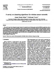
Figure 2.3: The location of the FS–interference caused by IEEE 802.11b to Bluetooth. has gained significant attention within the IEEE 802 working groups, such that a dedicated IEEE 802.19 Coexistence Technical Advisory Group (TAG) has been formed [19]. The task of IEEE 802.19 TAG is to “. . . develop and maintain policies defining the responsibilities of 802 standards developers to address issues of coexistence with existing standards and other standards under development . . . ”. A major work in the problem of coexistence has been conducted as a part of IEEE 802.15 standardization and a dedicated task group has developed the recommended practice for coexistence of WPANs with other wireless devices operating in the unlicensed spectrum [20]. The recommended practice addresses the issue of coexistence between IEEE 802.15.13 WPANs and IEEE 802.11b WLAN with direct sequence spread spectrum (DSSS) [21, 22, 23], as both of them are operating in the ISM band. The standard contains models of interference between WLAN and WPAN and specifies several coexistence mechanisms to overcome this interference. From a viewpoint of a Bluetooth piconet, a collocated IEEE 802.11b WLAN [24] can be regarded as an FS–interferer. As depicted on Figure 2.3, the FS–interference can occur at three different regions. The task group IEEE 802.15.2 defines two classes of coexistence mechanisms for WPAN and WLAN: collaborative and non-collaborative. In collaborative mechanisms the interfering entities exchange data to achieve mutual coordination, while non-collaborative mechanisms consider that data exchange is not available. The three collaborative mechanisms proposed in [20] are restricted by the requirement that the WPAN and WLAN are collocated within the same physical unit such 3 The

IEEE standard 802.15.1 is essentially based on the Bluetooth Specification and the terms “IEEE 802.15.1 WPAN” and “Bluetooth piconet” can be used interchangeably

18

CHAPTER 2. BACKGROUND ON FH NETWORKS that they can exchange information and coordinate each other within that unit. The non–collaborative techniques applied by the piconet can be classified as adaptive packet selection/scheduling and Adaptive Frequency Hopping (AFH). Besides having such techniques specified in [20], there has been a large volume of related research [25, 26, 27]. From the WPAN viewpoint, this is the case of FS–interference, such that the non–collaborative mechanisms avoid the interference with the strategy of bad channel removal i.e. the WPAN avoids to use the channels when FS–interference is present. For that purpose, the non-collaborative techniques perform classification of channels as “good or “bad”, corresponding to low or high interference. The classification schemes recommended in [20] rely on Received Signal Strength Indication (RSSI), Packet Error Rate (PER) and/or carrier sensing. The method relying on PER is by far the simplest one, since the RSSI method requires baseband processing while the carrier sensing introduces hardware changes. In adaptive packet scheduling the packet type and the transmission timing are adapted to the channel conditions [25] [28]. AFH dynamically changes the hopping set, shortly hopset, such that the WPAN preferably hops over the set of good channels. Such AFH mechanism is incorporated into the latest Bluetooth specification [7]. All current AFH proposals [7, 20, 26, 27] rely on the strategy of bad channel removal, which is quite simple and straightforward. With this strategy, referred to as standard AFH, the WPAN suspends the usage of the channels that are assessed as “bad” for a certain time. The removed channels can be brought again to the active hopset after a timeout and re–assessed [7, 29]. The AFH schemes differ in a way this standard AFH strategy is implemented: how the channel classification is done, criterion for channel removal, timeout for reassessment etc. The standard AFH strategy cannot be classified as a conflict resolution, since the interfering entity is assumed not to actively participate in the avoidance of interference. In fact, the standard AFH strategy is not designed to mitigate the interference between FH networks. In addition to the research as well as the standardization activities related to WLAN / WPAN coexistence, a large volume of research has been dedicated to evaluate the self–interference among collocated Bluetooth piconets by analysis, simulation or experimentally [30, 31, 32, 33, 34, 12, 35, 36, 37, 14, 38, 39, 15, 40, 41, 42, 43, 44, 45]. The mechanisms to avoid the self–interference among the piconets can also be classified as collaborative and non–collaborative, depending on whether the piconets exchange information to support the self–interference avoidance. Collaborative mechanisms for avoidance of inter–piconet interference are applied to a scatternet in [13] and [46], but they do not provide mechanisms to completely avoid the self–interference, as it is the case with the SIA algorithms proposed here. Furthermore, in contrast to SIA mechanisms, the target of [13] and [46] is not the energy–efficient scatternet operation. 19

CHAPTER 2. BACKGROUND ON FH NETWORKS Non–collaborative mechanisms for coexistence among collocated piconets have been considered in [47], [48] and [49]. The basic approach in [47] and [48] is identical. In both papers the authors consider scenarios in which the Bluetooth piconet is interfered by a collocated WLAN and collocated piconets. The main idea is to use hybrid scheme for avoiding the interference: AFH to avoid the FS– interference from the WLAN and Listen–Before–Talk (LBT) to avoid the self– interference among the piconets. Recall that, in order to apply LBT, a carrier sensing ought to be implemented in the Bluetooth transceiver. The LBT mechanism introduces suppression of packet transmissions to avoid collisions. This introduces decrease of the throughput as compared to the case when the collocated piconets are using orthogonal hopsets, which is achieved by the AFR and DAFH mechanisms. On the other hand, both AFR and DAFH mechanisms can use carrier sensing to achieve the orthogonalization of the hopsets and this will be outlined in the algorithm descriptions. It is worth mentioning that the authors in [47] and [48] show the gain of the hybrid scheme for very large number of self-interfering piconets (> 10 and up to 200). Finally, an attempt to assign orthogonal hopsets to collocated piconets has been pursued in [49]. The authors refer to the FCC regulation [50] (see section 4.2). As opposed to the design of AFR, the authors interpret the regulation in the most straightforward manner and partition the set of 79 channels into five orthogonal hopsets such that each hopset contains at least 15 channels. In such case, there can be at most five collocated piconets free of self–interference. Furthermore, the hopsets are pre–assigned randomly to each piconet and there is no mechanism to adaptively partition and assign the hopset, as it is the case with DAFH.

20

Chapter 3 Distributed Algorithms for Self–Interference Avoidance (SIA) in Bluetooth Scatternets 3.1

Introduction and Motivation

A Bluetooth scatternet is a networking structure which provides interconnection of multiple piconets. Two piconets are said to be directly connected if there is a device that is member of both piconets. The Bluetooth Specification defines Participant in Multiple Piconets (PMP) as “a device that is concurrently a member of more than one piconet, which it achieves using time division multiplexing (TDM) to interleave its activity on each piconet physical channel”([7], Vol. 1, p. 18). We will refer to the PMP as to a bridge device, due to the function of PMP to relay traffic between piconets. This manner of interconnection is modular, such that a scatternet can be regarded as an extendable clustered network and a piconet as a cluster. When a bridge device is active in piconet πk , it tunes to the native clock of the master of µk and uses the BD_ADDR of µk to generate the correct hopping sequence. The bridge device can be master in one piconet and slave in the other piconets of which it is a member, or it can be slave in all piconets of which it is a member. A great deal of research has been dedicated to the problem of scatternet formation (see [51] and the reference therein), formulated as follows: Having a set of devices within physical proximity, how are the roles of masters, slave and bridges chosen, such that a connected scatternet with required features is obtained? The often considered scenario is the one in which the devices are physically equivalent with respect to their Bluetooth capabilities, so that the master and slave states are purely logical. This is a defining scenario for ad hoc networking, where the 21

CHAPTER 3. SIA IN BLUETOOTH SCATTERNETS network is created from scratch, without relying on pre–existing infrastructure. In our work, we will assume that the scatternet is already formed, roles to the devices are assigned and we focus on the issues related to the subsequent scatternet operation. The clocks of different masters are not mutually synchronized. The physical area is covered by multiple piconets and the piconets are necessarily spatially overlapped to a high degree. The fact that the piconets are interconnected into scatternet does not affect the time synchronization and hopping sequence applied in each piconet. Thus, each master continues to determine the hopping sequence independently, according to its address and native clock. This implies that the conflicts among the piconets occur in identical manner as if the spatially overlapped piconets are not interconnected. For the Bluetooth scatternet, we consider scenarios in which the Bluetooth devices can exhibit a very small (or not at all) mobility over a long period. In other words, the scatternet is deployed in a quasi-static manner: Once the device roles are decided and the network is formed, the scatternet retains its physical and logical configuration for a longer time. These scenarios can occur in some sensing/monitoring applications, collaborative computing etc. In such cases, the graceful degradation introduced by the self-interference among the piconets is definitely harmful within a long period. Therefore, regarding the scatternet formation, some authors [52] suggest that it is desirable to minimize the number of piconets, since a large number of piconets will incur more collisions. However, the decrease in the number of piconets may cause poor connectivity in the scatternet and traffic bottlenecks. The collisions and packet errors lead to packet retransmissions, which increases the amount of energy spent per useful data portion. Since the Bluetooth devices are battery-powered, economic utilization of the battery energy is of crucial importance, remarkably in the cases where the energy is not renewable (e.g. sensor applications). In this chapter we introduce distributed mechanism for self–interference avoidance (SIA) in a Bluetooth scatternet, by which the scatternet achieves energyefficient operation at the expense of minor degradation of the nominal throughput. We will first introduce the design framework and objectives in Section 3.2. The basic SIA mechanism is introduced in Section 3.3, along with the analytical treatment of the expected gain brought by the usage of the SIA algorithm. The next two sections treat the practical implementation of the SIA mechanism. Section 3.4 describes the initialization needed to support the SIA operation. Section 3.5 introduces the adaptive SIA (A-SIA) algorithm, which is designed such that the SIA operation adapts to the physical scatternet topology as well as to the actual interference pattern. The basic SIA mechanism assumes that each piconet is using the packets of identical and fixed length. In Section 3.6 this assumption is revised and the SIA mechanism is generalized by allowing the piconets using packets with different lengths. The last section summarizes the chapter. 22

CHAPTER 3. SIA IN BLUETOOTH SCATTERNETS

3.2

Framework for Self–Interference Avoidance (SIA) by Distributed Conflict Resolution

The interconnected piconets can exchange information through the scatternet. This is a key argument to resolve the inter–piconet conflicts by applying adaptive scheduling of the packet transmissions rather than adaptation of the hopset. Note that by avoiding hopset adaptation, we avoid the discussion of the compliance with the rules for unlicensed frequency hopping. We define the framework for the distributed SIA mechanism through advocating its target features. We also give a functional sketch of the mechanism, while the detailed formulation of the basic SIA mechanism is given in the next section. Let us introduce the following terminology. A scatternet that uses SIA algorithm will be called SIA–ON scatternet, while the scatternet without self-interference avoidance will be called SIA–OFF scatternet. The following list shows the features that are required from the SIA algorithm: Feature 1 The set of transmissions performed in SIA–ON scatternet should be a subset of all possible transmissions that can occur in the SIA–OFF scatternet. Feature 2 The SIA algorithm should be run in a distributed manner. Feature 3 The SIA algorithm should use localized criterions for avoidance of the self-interference. The Feature 1 ensures that SIA–ON scatternet never causes more interference in the ISM band than what SIA–OFF scatternet can make. The SIA algorithm achieves this feature by keeping the hopping sequence of each piconet unaltered, while suppressing some of the transmissions in order to avoid conflict. Features 2 and 3 are required to ensure scalability and flexibility of the SIA algorithm. The scalability refers to the linear increase of the complexity of SIA algorithm, run by each piconet, as the number of devices/piconets in the scatternet grows. The flexibility refers to the adaptability of the SIA algorithm to the changes in the scatternet, both with respect to adding/removing piconets and to the variable traffic in the piconets. Nevertheless, the potential for flexibility is not employed in the basic SIA mechanism and will be utilized in the adaptive version of the SIA algorithm in Section 3.5. Let us observe a scatternet consisting of six piconets, depicted on Figure 3.1. Assume that each device from the scatternet is physically in the transmission range of any other device. Note that the set of logical links obtained in the scatternet formation is only a fraction of links that are physically possible to establish among the devices. The packet transmission in piconet πk is conflicting with the packet 23

CHAPTER 3. SIA IN BLUETOOTH SCATTERNETS

p1 m1

m3

p6

m3 p 3

m6

m6

p5 m5

m2

m5

p2 m4 p4

m4

Figure 3.1: Example of scatternet that consists of 6 piconets. Only the logical master-slave links are depicted and such st of links is a subset of possible physical links among the devices. transmission in πl if the transmitted packets use the same frequency and they overlap in time (partially or completely). We will also denote this situation as “piconets πk and πl are conflicting”. Assume that for the scatternet on Figure 3.1, at some instant, the following occurs: (a) all the packet transmissions in π1 , π2 and π3 use the same frequency f1 and are thereby conflicting; (b) the packet transmissions in π4 and π5 are conflicting at frequency f2 where f2 6= f1 ; (c) π6 uses frequency f3 , where f3 6= f1 and f3 6= f2 . For a SIA-OFF scatternet, the conflicting transmissions cause collisions at the intended receivers and, most probably, only the transmission in piconet π6 at frequency f3 is successfully performed. The target regime of operation for the SIA algorithm is: If two or more packet transmissions are conflicting, then the conflicting piconets achieve consensus such that a packet transmission in only one piconet is performed. Our proposed SIA algorithm will exhibit slight suboptimality by allowing at most one piconet from a group of conflicting piconets to transmit. The rule for achieving consensus in distributed manner makes the protocol scalable and fair towards each piconet.

3.3

The Basic Self–Interference Avoidance Mechanism

In this section we will specify the basic SIA mechanism through the rules to which the piconets adhere to in order to avoid the self–interference. The basic SIA mech24

CHAPTER 3. SIA IN BLUETOOTH SCATTERNETS anism is discussed through the analytical results in order to obtain the expected gain brought by its application in the scatternet.

3.3.1 Assumptions and Definitions Consider a scatternet that consists of N piconets π1 , π2 . . . , πN and the respective piconet masters are denoted by µ1 , µ2 , . . . , µN . Let us first assume that each µk has the BD_ADDR and clock information for any other µl . The essential assumption for the basic SIA mechanism is that all piconets are using packets of identical and fixed length. This assumption implies that the knowledge of BD_ADDR and clock information of µk is sufficient to know the frequency that should be used in πk at any instant. In particular, if not stated otherwise, the piconets are assumed to use exclusively 1–slot packets. For the completeness, we state how this assumption can be instantiated in a scatternet. After the scatternet formation, each master will use the fact that its piconet is part of a scatternet in order to set the maximal length of the used packet to be 1. This can be done by using the LMP_max_slot packet with max_slots= 1. In the discussion of the basic SIA mechanism, we make the worst case assumptions about the self–interference in the scatternet: 1. Single–hop. The transmission from any device in the scatternet can interfere the reception of any other device in the scatternet. 2. Destructive collisions. Let a device D1 receive a packet at frequency fm . If any other transmission at fm occurs during the reception of the packet, D1 receives the packet incorrectly. Define a transaction in a piconet to be a sequence of MS–packet and the SM– packet from the addressed slave. The polling applied in Bluetooth piconet allows to consider the transaction to be a basic unit for two–way transmission of information in the piconet. The transaction is defined as successful if no error occurs in any packet which belongs to that transaction. The goal of the SIA mechanism is to provide each piconet only with successful transactions. The i−th transaction in πk is denoted by τ(k, i) and it consists of (2i)−th and (2i + 1)−th slot in πk . The transaction is represented by the frequencies used: i τ(k, i) = [ fM , fSi ]

(3.1)

i denotes the frequency used by the MS–packet, while f i denotes the where fM S frequency used by the SM–packet. The value of the transaction τ(k, i) is defined as: i V [τ(k, i)] = fM + fSi (3.2)

25

CHAPTER 3. SIA IN BLUETOOTH SCATTERNETS

 piconet πk

i fM

 piconet πl

j fM

transaction τ(k, i) fSi

τ(l, j) j fS

-

- 

τ(l, j + 1)

-

j+1 fM

Figure 3.2: Overlapping between the transactions of two piconets πk and πl A transaction is performed if the MS– and SM–packet are transmitted. Let us first assume that a MS– or SM–packet completely covers the whole slot i.e. we neglect the need for the turnaround time and the maximal duration of 1–slot packet is 625 µs instead of 366 µs. Figure 3.2 illustrates the overlapping between transactions in two piconets πk and πl . Since the piconets are not synchronized, each transaction in πk overlaps with two transactions in πl and vice versa. For the example in Figure 3.2, τ(k, i) overlaps with τ(l, j) and τ(l, j + 1), while τ(l, j) overlaps with τ(k, i) and τ(k, i + 1) (not shown). We define τ(l, j) to be the left overlap of τ(k, i) and τ(l, j + 1) to be the right overlap of τ(k, i). For a shorter notation, we use j = LOkl (i) and ( j +1) = ROkl (i). From symmetry, if j = ROkl (i) then i = LOlk ( j). Let the master µk know the left and right overlap in another piconet πl for some transaction τ(k, i0 ). If the clock drift is neglected, then µk knows the left and right overlap for all τ(k, i1 ) where i1 > i0 . Two overlapping transactions τ(k, i) and τ(l, j) are concurrent if there is a packet in τ(k, i) that should simultaneously use the same frequency with a packet i = f j or f i = f j or in τ(l, j). For Figure 3.2, τ(k, i) is concurrent with τ(l, j) if fM M M S j fSi = fS . If two concurrent transactions are performed, then there are conflicting packet transmissions and the assumption for destructive collisions implies that errors in both packet will occur. If τ(k, i) and τ(l, j) are concurrent, but only τ(k, i) is performed, then there is no conflict. Finally, we define the notion of usable transaction. The transaction τ(k, i) is usable with respect to the overlapping transaction τ(l, j) if either C1 or C2 is satisfied: C1: τ(k, i) and τ(l, j) are not concurrent; C2: τ(k, i) and τ(l, j) are concurrent and V [τ(k, i)] > V [τ(l, j)]. The transaction τ(k, i) is usable with respect to piconet πl if and only if τ(k, i) is usable with respect to both left and right overlap in πl . 26

CHAPTER 3. SIA IN BLUETOOTH SCATTERNETS start: set perform=true ; for(each πl , l 6= k); set j = LOkl (i); if (τ(k, i) is concurrent with τ(l, j)) then if (V [τ(k, i)] ≤ V [τ(l, j)]) then set perform=false ; set j = ROkl (i); if (τ(k, i) is concurrent with τ(l, j)) then if (V [τ(k, i)] ≤ V [τ(l, j)]) then set perform=false ; if (perform==true ) send (MS–packet ); receive (SM–packet ); else go to sleep mode until the start of the next transaction; set i = i + 1; goto start;

Figure 3.3: Pseudocode description of the SIA algorithm. This procedure is executed by the master µk prior to the start of i−th transaction in πk

3.3.2 Formulation of SIA algorithm Equipped with the above definitions, we can concisely state the basic SIA algorithm. The appropriate pseudocode is shown in Figure 3.3. Before starting τ(k, i), the master µk checks whether its transaction is usable with respect to all other piconets in the scatternet. If it is, then µk sends MS–packet and thereby starts the transaction τ(k, i). Conversely, if there is at least one piconet πk1 , such that τ(k, i) is not usable with respect to πk1 , then µk does not send MS–packet. Hence, no slave is polled and no SM–packet is sent, which makes the piconet πk silent during the time reserved for τ(k, i). At the start of the transaction τ(k, i) each slave in πk attempts to receive the header of the MS–packet in order to check whether it is being polled. If πk should be silent during τ(k, i), each slave finds out that it is not being polled and the Specification [7] prescribes that the slave should go to sleep until the next even slot i.e. until the start of the next transaction. The natural question here is—what happens with the master µk when πk should stay silent? In the SIA algorithm, the master puts its transceiver into sleep mode until the start of the next transaction. Such model of activity in the piconet has also been used in [35]. The overall effect is that the piconet saves energy instead of wasting it into a possibly erroneous transmission. In this form, the SIA algorithm assumes that each piconet has ACL traffic only, since in that case the master is not obliged to start a transaction. Although the SIA algorithm is intended for the ACL traffic, the SCO traffic can be easily ac27

CHAPTER 3. SIA IN BLUETOOTH SCATTERNETS commodated within this framework. The SCO transmissions must be performed. Then, if there is SCO traffic in some piconet, a device that has reserved a slot for SCO transmission simply ignores the SIA algorithm. It is essential to note that the condition C2 guarantees avoidance of conflicting packet transmissions in the scatternet when the SIA algorithm is applied by all member piconets. Let τ(k, i) and τ(l, j) be concurrent and let µk assess that τ(k, i) is usable with respect to τ(l, j). Then µl assesses V [τ(l, j)] < V [τ(k, i)] and µl decides that πl should stay silent during τ(l, j). Due to the pseudorandom selection of the frequencies, the condition C2 is fair: Over a longer interval, the expected number of times for which V [τ(l, j)] < V [τ(k, i)] is equal to the expected number of times for which V [τ(l, j)] > V [τ(k, i)]. The SIA algorithm ensures that at most one transaction is executed when there is concurrence, which can sometimes lead to suboptimal behavior. One possible suboptimality occurs as follows: Let τ(k, i) and τ(l, j) be concurrent due to, for exi = f j . Then, if f i = f j , both µ and µ calculate V [τ(l, j)] = V [τ(k, i)] ample, fM k l M S S and both πk and πl stay silent during τ(k, i) and τ(l, j), respectively 1 . There is a simple way to repair this suboptimality2 , at the expense of slight unfairness: Whenever the values of the concurrent transactions are identical, the master with higher value of BD_ADDR claims its transaction usable. This rule would give slightly higher throughput to the masters with higher addresses. Another suboptimal behavior results from the fact that SIA does not consider global information over the scatternet and also it does not memorize the transaction assessments. For assessing the the usability of τ(k, i) the master µk does not rely on the assessments of τ(k, i1 ) where i1 < i. Take the example on Figure 3.4: 1. τ(1, i1 ) is not usable with respect to τ(2, i2 ) 2. τ(2, i2 ) is not usable with respect to τ(3, i3 ) 3. τ(3, i3 ) is not usable with respect to τ(1, i1 + 1) If SIA from Figure 3.3 is applied, then neither of τ(1, i1 ), τ(2, i2 ), τ(3, i3 ) is performed. Note that in this case µ1 can see in advance the facts stated by 2. and 3. 1 According

to the most recent Bluetooth Specification [7], if the piconet operates in mode of enabled Adaptive Frequency Hopping, then the the frequencies of the MS– and SM–packet from the same transaction are identical. The nominal frequencies of the transaction τ(k, i) = [ fMi , fSi ] are unaltered, only the slave forces the usage of the frequency fMi for the SM–packet. In this case the SIA-mechanism can be straightforwardly applied: To determine the concurrency, the transaction is observed through the frequencies that are to be used for transmission, i.e. τ′ (k, i) = [ fMi , fMi ], while to break the ties upon concurrency, the nominal transaction value V [τ(k, i)] = fMi + fSi is used. In this chapter we consider that the slave always uses the nominal pseudorandom frequency for transmission, without forcing usage of the frequency fM for the SM–packet 2 However, in our analysis and implementation of SIA we do not use this “repairing”.

28

CHAPTER 3. SIA IN BLUETOOTH SCATTERNETS  π1

-  τ(1, i1 + 1) τ(1, i1 ) freq= 10 37 56 62 

π2

10

53

 π3

-

τ(2, i2 )

-

τ(3, i3 ) 53

56

Figure 3.4: An example of suboptimal behavior of the SIA algorithm. A number denotes the frequency used in that slot. Neither of the transactions τ(1, i1 ), τ(2, i2 ), τ(3, i3 ) is assessed as usable. above and it can claim τ(1, i1 ) usable. Conclusively, by introducing memory (or look–ahead) in the SIA algorithm and observing global state in the scatternet, the throughput can be further improved. However, this improvement comes at the expense of much increased complexity. Namely, instead of checking the transaction with respect to each piconet separately, in this case the piconet should account for how the other piconets have assessed their transactions. This is exactly what we want to avoid in order to achieve scalability. Besides the scalability, the proposed SIA algorithm possesses the other two desired features from Section 3.2. Since some of the possible transactions are suppressed, the resulting set of performed transactions in SIA–ON scatternet is a subset of possible transactions in the corresponding SIA–OFF scatternet. Furthermore, the SIA mechanism is run distributedly, while the transaction is assessed via local (piconet–to–piconet) assessments and is localized in time (no memory). The Impact of Partially Loaded Slots Hitherto we have assumed that a single slot packet has duration equal to the whole slot, 625 µs. According to the Bluetooth specification, the maximal length of a single slot packet can be 366 µs. Some packets, such as POLL or NULL are even shorter than 366 µs. Let us denote by r = TTPS the fill factor of a packet, where TP is the packet duration and TS is the slot duration. The smaller the fill factor, the lesser the self–interference in an SIA–OFF scatternet. Figure 3.5 illustrates how a fill factor r < 1 should affect the SIA algorithm. For this particular choice of ∆lk , each transaction in πk overlaps only with a single transaction in πl i.e. πk has only a left overlap in πl . Therefore, if µk has a precise value of ∆lk it assesses the usability of τ(k, i) only with respect to τ(l, j), but not with respect to τ(l, j + 1). The SIA algorithm that assumes that each piconet knows the precise slot offsets with respect to all other piconet will be referred to as 29

CHAPTER 3. SIA IN BLUETOOTH SCATTERNETS

∆lk

↔



piconet πk

i fM

 piconet πl

-

τ(k, i) fSi

- 

τ(l, j)

j

j

fM

fS

τ(l, j + 1)

j+1

fM

Figure 3.5: Overlapping between the transactions of two piconets πk and πl when a packet does not fill the slot completely. SIA with perfect timing. The value r < 1 decreases the self–interference in a SIA– OFF scatternet, but it also increases the probability of getting usable transaction when SIA–PT algorithm is run. However, due to the clock drift, it is not reasonable to assume perfect knowledge of the slot offsets at any instant. Therefore, each piconet runs the SIA algorithm as described previously, by making the pessimistic assumption that a slot is completely filled by packet. In order to stress that the slots have r < 1, but the SIA algorithm treats them as r = 1, we refer to this algorithm as SIA with imperfect timing. In this thesis we will adopt and analyze only SIA with imperfect timing. It is important to note that the basic SIA algorithm can be directly applied in the case when all piconets in the scatternet are using either only 3–slot packets or only 5–slot packets. Let us assume that all piconets are always using only 3– slot packets and analogous discussion applies to the case with 5–slot packets only. Then each transaction lasts for 6 slots and overlaps with at most 2 transactions in 366 another piconet. In such case the fill factor is higher r = 2·625+366 = 0.862 > 625 = 3·625 0.5856. However, if solely 3–slot packets are used, it is unrealistic to assume that each “container” for 3–slot packet will be always maximally filled with data. Furthermore, in such case the SCO traffic cannot be seamlessly supported as in the case of exclusive usage of 1–slot packets.

3.3.3 Analysis of the Basic SIA Algorithm Throughput Analysis for the SIA–OFF scatternet In order to model the piconet behavior, we make the following assumptions. In each slot the frequency is chosen independently and uniformly from the set of F frequencies. Regarding the traffic model, in each even slot a transaction is started with probability G, where G is referred to as activity factor. Each transaction contains both an MS– and an SM–packet. This is slightly different from the model 30

CHAPTER 3. SIA IN BLUETOOTH SCATTERNETS Case Error Description 1 Error in the header of the 2 3 4 5

MS–packet Error in the MS–payload, no error in the SM–packet Error in the MS–payload, error in the SM–packet No error in the MS–packet, error in the SM–header No error in the MS–packet, error in the SM–payload

Effects on information transmission The slave does not detect that is being polled and does not transmit SM–packet Data transmitted from slave to master, slave waits for acknowledgement No data is transmitted The master assumes that its packet has been lost and retransmits it subsequently Data transmitted and acknowledged from master to slave

Table 3.1: The effect of packet errors on a transaction in a piconet used for analysis in, e.g. [12], where a slot can contain a packet with probability G, independently of the other slots. The actual effect of the errors on the data transmission through the piconet transactions is shown by the Table 3.1. This renders our traffic model approximate. For example, note that in Case 1 the SM–packet is not transmitted, while in our model we have assumed that the SM–packet always follows the MS–packet. In our model we will assume that a packet that has been successfully transmitted is not retransmitted. Regarding the case 4 of Table 3.1, it follows that our model upperbounds the throughput in the SIA–OFF scatternet. The pattern by which the transactions of two piconets overlap depends on the slot offset ∆lk , as shown on Figure 3.6. The piconet πk is a reference piconet and πl is an interfering piconet. The other quantities are: • TS - slot duration of 625 µs. • TP - packet duration, 366 µs for 1–slot packets. The packet offset ∆ = ∆lk obtains values from the interval [0, 2TS ). Noting that TP > T2S , we can identify 4 different regions within [0, 2TS ) which yield different overlap between the transactions/packets of πk and πl . Table 3.2 shows this overlap. For convenience, the MS–packet of the observed transaction in πk is denoted only by fM , and the SM–packet by fS . For example, in region [TS − TP , TP ), the MS–packet in πk overlaps with both the MS– and the SM–packet of a same transaction in πl , while the SM–packet in πk overlaps with SM–packet of one transaction and the MS–packet of the next transaction. Let QM (Ii ) denote the probability of successful transmission of MS–packet in πk when ∆ ∈ Ii . Similarly, QS (Ii ) denotes the success probability for an SM– packet in πk . For ∆ ∈ I1 or ∆ ∈ I3 , each packet overlaps with only one packet, such 31

CHAPTER 3. SIA IN BLUETOOTH SCATTERNETS Region for ∆ I1 = [0, TS − TP ) ∪ [TS + TP , 2TS ) I2 = [TS − TP , TP ) I3 = [TP , 2TS − TP ) I4 = [2TS − TP , TS + TP )

Overlap of fM fM ( j) fM ( j), fS ( j) fS ( j) fS ( j), fM ( j + 1)

Overlap of fS fS ( j) fS ( j), fM ( j + 1) fM ( j + 1) fM ( j + 1), fS ( j + 1)

Table 3.2: List of the overlapping between the packets of two piconets for different values of the slot offset that: QM (I1 ) = QM (I3 ) = QS (I1 ) = QS (I3 ) = 1 −

G F

(3.3)

For ∆ ∈ I2 we have:  1 2 (3.4) QM (I2 ) = (1 − G) + G 1 − F   G 2 QS (I2 ) = 1 − (3.5) F The difference between (3.4) and (3.5) comes from the fact that either the MS– packet overlaps with 2 packets (if there is transmission in the corresponding transaction of πl ) or with none. On the other hand, the SM–packet overlaps with two packets, each of which is independently generated with probability G. This situation is reversed for ∆ ∈ I4 , such that:   G 2 QM (I4 ) = 1− F   1 2 QS (I4 ) = (1 − G) + G 1 − (3.6) F 

∆lk

↔ TS  TP piconet πk

piconet πl

-

i fM

j

fSi

j

fM

fS

Figure 3.6: Overlapping between the packets of the reference piconet πk and the interfering piconet πl . 32

CHAPTER 3. SIA IN BLUETOOTH SCATTERNETS Let the value of ∆ be uniformly distributed in [0, 2TS ). Let QM and QS denote the probabilities of successful transmission of an MS–packet and an SM–packet, respectively, in the reference piconet πk , when there is only a single interfering piconet. Then, taking QM (∆) to be the probability of success for given ∆ and averaging over ∆: Z

2TS

1 d∆ = 2TS 0 2(TS − TP ) 2TP − TS 2TP − TS = QM (I1 ) + QM (I2 ) + QM (I4 ) TS 2TS 2TS

Q = QM =

QM (∆)

(3.7) (3.8)

Clearly, QS = QM = Q. For the SIA–OFF scatternet that consists of N piconets, under all stated assumptions, the probability of successful packet transmission in a single piconet is: QM,N = QS,N = QN−1 = QN (3.9) assuming that G is identical for all piconets. Denoting the data rate of the 1–slot packet by R1 , the throughput in a single piconet of the SIA–OFF scatternet is: SOFF,N = G · QN · R1

(3.10)

Throughput Analysis for the SIA–ON scatternet When SIA algorithm is applied, the quantity of interest is the fraction of all transactions within πk which are assessed as usable and are at disposal for packet transmission. Let PN (u) denote the probability that a transaction is assessed usable when there are N piconets in the scatternet. When there is only one interfering piconet, we use the notation P2 (u) = P(u). Then: PN (u) = (P(u))(N−1)

(3.11)

Note that the value of P(u) does not depend on the activity factor G in the piconets. Due to the imperfect timing, the master in πk that runs the SIA algorithm always assumes that each of its transactions overlaps with two transactions in another piconet πl . In such case there are two different patterns of overlapping. i overlaps with Figure 3.2 depicts one of the patterns, while in the other pattern fM j−1 j j j fS and fM , while fSi overlaps with fM and fS . The value of P(u) is identical for both cases, such that we analyze only the pattern from Figure 3.2. Let Pi, j (u) ¯ denote the probability that the transaction τ(k, i) is not usable with respect to τ(l, j). Analogously, we define Pi, j (u) = 1 − Pi, j (u). ¯ The probability Pi, j (u) ¯ can be represented as: F

Pi, j (u) ¯ =

∑P

f =1



j fS

  j = f · P u| ¯ fS = f

33



(3.12)

CHAPTER 3. SIA IN BLUETOOTH SCATTERNETS   j j where P fS = f = F1 is the probability that fS is equal to a particular frequ  j ency f . P u| ¯ fS = f is the conditional probability that τ(k, i) is not usable when   j P fS = f and is calculated as: j

j

P(u| ¯ fS = f ) = P( fSi < f ) · P(u| ¯ fS = f , fSi < f ) + j

+P( fSi = f ) · P(u| ¯ fS = f , fSi = f ) + j

+P( fSi > f ) · P(u| ¯ fS = f , fSi > f )

(3.13)

j

since P( fSi = f0 ) = P( fSi = f0 | fS = f ) due to independence. We consider each summand of (3.13) separately: j

1. Case fSi < f = fS .

f −1 F From the rules of the SIA algorithm it follows that in this case τ(k, i) bei = f j , such that comes unusable with respect to τ(l, j) if fM M P( fSi < f ) =

j

j

i P(u| ¯ fS = f , fSi < f ) = P( fM = fM ) =

1 F

(3.14)

j

2. Case fSi = f = fS . j

j

P(u| ¯ fS = f , fSi = f ) = 1 − P(u| fS = f , fSi = f ) F −1 j j i P(u| fS = f , fSi = f ) = P( fM > fM ) = 2F which implies j

P(u| ¯ fS = f , fSi = f ) =

F +1 2F

(3.15)

j

3. In the case fSi > f = fS , τ(k, i) is always usable with respect to τ(l, j), rei and f j . Then gardless of the relation between fM M j

P(u| ¯ fS = f , fSi > f ) = 0

(3.16)

Using (3.14-3.16), the equation (3.13) becomes: j

P(u| ¯ fS = f ) =

1 f −1 1 F +1 · + · F F F 2F 34

(3.17)

CHAPTER 3. SIA IN BLUETOOTH SCATTERNETS and the probability in (3.12) becomes:   F 1 F +1 f −1 1 + 2 Pi, j (u) ¯ = ∑ · = 2 2F F F f =1 F

(3.18)

From Figure 3.2, τ(k, i) also overlaps with τ(l, j + 1). In this case: j+1

j+1

i Pi, j+1 (u) ¯ = P( fSi = fM ) · P( fM ≤ fS

j+1

| fSi = fM ) =

1 F +1 · F 2F

(3.19)

The probability to have a usable transaction in SIA–ON scatternet that consists of two piconets is:   

F +1 1 1− (3.20) P(u) = 1 − Pi, j (u) ¯ 1 − Pi, j+1 (u) ¯ = 1− F 2F 2

which can be used in (3.11) to obtain the value for SIA–ON scatternet with N piconets. The maximal throughput in a piconet which is member of such scatternet is: SON,N = PN (u) · R1 (3.21) Energy Model and Energy Efficiency Based on Table 3.1 and the analysis in the previous two subsections, we can build an approximate model for the energy consumption in a piconet. Let the volume of data that should be exchanged in the piconet consist of D transactions i.e. D 1–slot MS–packets and D 1–slot SM–packets. By analogy with [53] we define the energy–efficiency as: D (3.22) η= Et where Et is the total energy used by the piconet to transmit the useful data volume. Let ET X and ERX denote the energies for transmission/reception of a single–slot packet, respectively. Let EH be the energy needed to receive only the packet header. The energy consumed in sleep and idle mode is taken to be zero. The energy consumed in a piconet with U slaves during a single transaction in which both MS–packet and SM–packet are transmitted is: Etran = 2(ET X + ERX ) + (U − 1)EH

(3.23)

where (U − 1)EH is the contribution from the non–addressed slaves which listen only to the header of the MS–packet. If the master does not initiate transaction by sending an MS–packet, the piconet stays silent, but some energy is still consumed. The slaves listen for a header of an MS–packet, after which they go to sleep until 35

CHAPTER 3. SIA IN BLUETOOTH SCATTERNETS the next even slot. The energy consumed in the piconet during a silent transaction is: Esilent = U · EH (3.24) Let us first consider a piconet from a SIA–OFF scatternet within a time interval that has a duration of V transactions. According to the assumed traffic activity model for a piconet, G ·V transactions are not silent such that the energy spent in the piconet during the observed time is: EOFF = G ·V · Etran + (1 − G) ·V · Esilent

(3.25)

If the data volume D and activity factor G are given, we can determine V . Having in total 2D MS– and SM–packets, the following equation should hold: 2D = 2G ·V · Q2N + G ·V · QN (1 − QN ) + G ·V · QN (1 − QN ) = = G ·V · QN (3.26) where QN is given by (3.9). Consequently: V=

2D G · QN

(3.27)

The equation (3.26) comes from the fact that Q2N is the probability that both MS– and SM–packet are transmitted successfully, while QN (1 − QN ) is the probability that either MS– or SM–packet is transmitted successfully. Using (3.25) and (3.27), the energy efficiency in a SIA–OFF scatternet with N piconets can be calculated as: G · QN ηN (SIA-OFF) = (3.28) G · Etran + (1 − G) · Esilent Since we assume that errors can only occur due to the self–interference, a piconet in the SIA–ON scatternet never retransmits a packet. Hence, for the same amount of useful data transmitted, a piconet in the SIA–ON scatternet should have lower activity factor as compared to the piconet from an SIA–OFF scatternet. For a fair comparison, we assume that in the piconet from the SIA–ON scatternet within the same observation interval of V transactions there has been in total 2D = G · QN ·V packets transmitted, according to (3.27). The equivalent activity factor for the SIA–ON scatternet is Ge = G · QN such that for the energy efficiency it can be written: ηN (SIA-ON) =

G · QN G · QN · Etran + (1 − G · QN ) · Esilent

36

(3.29)

CHAPTER 3. SIA IN BLUETOOTH SCATTERNETS

3.3.4 Analytical Results and Expected Gain Introduced by the SIA Mechanism In this section we will show the results from the presented theoretical analysis. Considering the radio range of the Bluetooth system, we put N = 30 to be the maximal number of piconets that can self–interfere destructively.3 If not explicitly stated otherwise, the number of frequency channels is F = 79. A piconet that is a member of SIA–OFF or SIA–ON scatternet will be shortly referred to as SIA– OFF or SIA–ON piconet, respectively. Figure 3.7 shows the maximal throughput that can be obtained for a SIA– OFF and SIA–ON piconet, respectively. The throughput of the SIA–OFF piconet has been plotted for 4 different values of the fill factor r. Due to the imperfect information, the performance of the SIA–ON piconet does not depend on the fill factor. The throughput is normalized 4 by taking the value R1 in (3.10) and (3.21) to be R1 = 1. The maximal throughput SOFF,N in SIA–OFF piconet according to (3.10) is obtained by setting G = 1. The maximal throughput SON,N = PN in SIA– ON piconet is obtained when there are transmissions in all usable transactions, according to (3.21). The fill factor r = 0.586 corresponds to the usage of a 1– slot packet. We have already stated in subsection 3.3.2 that the SIA algorithm can be straightforwardly used if all piconets in the scatternet use exclusively 3– and 5–slot packets. The usage of solely 3–slot packets corresponds to fill factor r = 0.862, while the usage of solely 5–slot packets corresponds to r = 0.917. As a reference, we have plotted SOFF,N = QN for a fill factor r = 1. The assumption that the piconets have G = 1 has a practical interpretation. Consider a sensor network in which the activation of the piconets may occur in correlated manner – after a fairly long time of inactivity, the scatternet may enter into a relatively short interval of intensive activity. When the traffic activity in the piconets has a temporal correlation, it is viable to assume that an interfering piconet always has a data to start a transaction (G = 1). It can be seen that the attainable QN with r = 0.586 is higher than PN for any number of piconets N. On the other hand, for the other three fill factors, QN is smaller than PN . Recall that we use SIA with imperfect timing information, such that a master in SIA–ON piconet always makes a pessimistic assumption about the interference with another piconet: The transaction might be claimed unusable even if there is no actual overlapping between the packets of the different piconets. As the fill factor increases, the impact of the imperfect timing information on the 3 In

some other theoretical investigations in the literature the upper bound on the number of self–interfering piconets has been taken much higher, e.g. 50 in [12] and 200 in [15]. 4 The actual value when only DH1 packets are used would be 345.6 kbps, which is a two–way goodput value: If both MS– and SM–packet of a transaction are successfully transmitted, then in total 2 · 27 bytes of data are transferred within the piconet during 2 · 625µs

37

CHAPTER 3. SIA IN BLUETOOTH SCATTERNETS

Normalized throughput per piconet

1

0.9

0.8

0.7

0.6

0.5

0.4 0

5

10

SIA-OFF, r=0.586 SIA-OFF, r=0.862

15 Number of piconets N

20

SIA-OFF, r=0.917 SIA-OFF, r=1

25

30

SIA-ON

Figure 3.7: Maximal achievable throughput for a piconet in SIA–OFF and SIA– ON scatternet. The results for SIA–OFF piconet are shown for two different values of the fill factor r. throughput of a SIA–ON piconet decreases. For the cases when piconet activity is G < 1 and QN > PN , the packet delay incurred by the usage of the SIA algorithm slightly increases. Since the delay itself is not of a major interest here, we discuss it in Appendix B, where we show the analytical relations between the throughput and delay. These results may suggest that, to avoid throughput loss, the SIA algorithm should always be applied by using exclusively 3– or 5–slot packets in all SIA–ON piconets. Nevertheless, these values of QN are obtained if all 3–and 5–slot packets have maximal length. Thus, one has to be cautious about such conclusion when realistic traffic patterns in a piconet are considered, which in turn depends on: the packet arrivals at the piconet devices, the scheduling that the master applies to poll the slaves and the routing of the data throughout the scatternet. The relation of the SIA mechanism to the packet length is further discussed in Section 3.6. In order to evaluate the energy efficiency, we use the same energy model as in [54], ET X = 2ERX and EH = E6RX . Figure 3.8 depicts the energy ratio: ρN =

ηN (SIA-OFF) · 100[%] ηN (SIA-ON)

(3.30)

where ηN (SIA-OFF) and ηN (SIA-ON) are given by (3.28) and (3.29), respectively. For given scatternet size N, the energy ratio ρN indicates which percentage of the energy used in SIA–OFF piconet should be used by a SIA–ON piconet for transmission of the same amount of data. Hence, the lower ρN the higher the 38

CHAPTER 3. SIA IN BLUETOOTH SCATTERNETS 100 95 90

Energy ratio [%]

85 80 75 70 65 60 55 50 45 5

10

15 20 Number of piconets N

r=0.586, U=1 r=0.586, U=7

25

30

r=1, U=1 r=1, U=7

Figure 3.8: Energy ratio ρN between the energy efficiencies of the SIA–OFF and SIA–ON scatternets. G = 1. For each fill factor r, ρN is evaluated for two different values of the number of slaves U.

gain from the usage of the SIA algorithm. The energy ratio is depicted versus the number of piconets in the scatternet. The activity factor is G = 1. As with the throughput, here the higher fill factor r yields again better performance of the SIA algorithm. For the same fill factor, having higher number of slaves decreases the energy ratio. This is because the overall energy spent for listening the packet headers increases both in SIA–ON and SIA–OFF piconet. Figure 3.9 shows the dependency of the energy ratio on the activity factor G for two different scatternet sizes. As G decreases, the energy ratio increases, which decreases the overall gain of using the SIA algorithm. The dependency of energy ratio on the number of frequency channels (hopset size) F used by the piconets is depicted on Figure 3.10. The motivation to show these results comes from the possible application of adaptive frequency hopping (AFH) in the piconets according to the Bluetooth Specification [7]. If the scatternet is deployed in vicinity of a 802.11 WLAN or other interferer, then AFH may cause reduction of the hopset for all piconets in the scatternet. Figure 3.10 shows the energy ratio for two sizes of the reduced hopset F = 40 and F = 20. For smaller hopset sizes the collisions among piconets become more probable, which implies that more energy is wasted in the SIA–OFF scatternet. Hence, the collision–free operation offered by the SIA algorithm is beneficial and the energy ratio becomes very low for small F. 39

CHAPTER 3. SIA IN BLUETOOTH SCATTERNETS

1 0.95

Energy ratio [%]

0.9 0.85 0.8 0.75 0.7 0.65 0.6 0.1

0.2

0.3

0.4

0.5 0.6 0.7 Piconet activity factor G

N=10, r=0.586 N=10, r=1

0.8

0.9

1

N=20, r=0.586 N=20, r=1

Figure 3.9: Energy ratio ρN between the energy efficiencies of the SIA–OFF and SIA–ON scatternets for two different scatternet sizes and two different fill factors r. The number of slaves is U = 1.

100 90 80

Energy ratio [%]

70 60 50 40 30 20 10 5

F=79

10

15 20 Number of piconets N F=40

25

30

F=20

Figure 3.10: Energy ratio ρN for three different hopset sizes. G = 1 and r = 0.586.

40

CHAPTER 3. SIA IN BLUETOOTH SCATTERNETS  πk

τ(k, i) 2i 2i + 1

πl

τ(l, j − 1) -  τ(l, j) 2j−1 2j  ∆kl -

Figure 3.11: Offset information for two piconets. ∆kl is the slot offset. The number in each time slot denotes the clock value of the appropriate master for that slot.

3.4

Initialization of the SIA Mechanism

The SIA mechanism is initialized in a distributed and asynchronous way. The piconets need not start the SIA algorithm simultaneously and it is only required that each master eventually gets the clock from all other masters in the scatternet. After receiving for the first time the clock/address information about some µl , the master µk start to check usability of its transactions with respect to µl . To summarize, the collisions due to self–interference in a SIA–ON scatternet are possible only as long as there is at least one µk1 that has not received the clock/address information from all other masters in the scatternet. An important element of the SIA algorithm is that each master should broadcast its clock/address information to all other masters in the scatternet. Let us call the packet that carries such information CA–packet. The detailed design of the broadcast protocol is out of scope for this work and it can rely on some current solutions for routing and broadcasting in scatternets [55]. Here we are focused on the design of the packet that should be broadcasted and how it should be updated upon rebroadcasting. Figure 3.11 depicts the information that should be known for µk to run the SIA algorithm with respect to πl . The value ∆kl is defined in the Bluetooth Specification as slot_offset and is expressed in microseconds. Since the duration of each transaction is 2 · 625 = 1250 µs, it follows that ∆lk = 1250 − ∆kl . In order to run the SIA algorithm when a slot is completely filled by a packet, for the example on Figure 3.11 µk needs only to know that during the 2i−th slot of πk , the piconet πl makes transition from slot (2 j − 2) to slot (2 j − 1). Note that in this case the exact value of ∆kl is not needed for the actual execution of the SIA algorithm. Once µk determines that τ(l, j) is the right overlap of τ(k, i) and assuming that the clocks are not drifting, µk obtains the right overlap τ(l, j′ ) for some τ(k, i′ ), where i′ > i as j′ = j +(i′ −i). The calculation of the hopping sequence for another piconet is not a computational burden for the master. The master µk can reuse its 41

CHAPTER 3. SIA IN BLUETOOTH SCATTERNETS built–in generator for hopping sequence and compute the hopping sequence of πl by setting the clock and address of µl as an input. Forwarding of CA–packets The scatternet–wide broadcast of the CA–packet from some master µk requires active forwarding by the masters and slaves. Here we design the broadcast of CA–packets by using unicast master–slave links of the piconets as well as the information provided by the standard packets defined in the Bluetooth Specification. In order to define the type of information contained in the CA–packet, we note that the broadcast takes part above the link layer of Bluetooth. Hence, in defining the CA–packet we speak about nodes, without differentiating masters and slaves, although the originator source of the CA–packet is always a master. Let us observe a CA–packet originated from the node dk . When a node dl receives that CA–packet, it should extract the following information from the packet: • BD_ADDR of the originator dk • An even number il ≥ 0, denoted as destination slot • The unique even number ik ≥ 0, denoted as originator slot, with the following feature: The slot number ik in πk starts ∆lk < 1250 microseconds after the start of slot il in πl . • The slot offset ∆lk . Let us observe 3 devices d1 , d2 , d3 (Figure 3.12). Let device d1 be master in π1 and d2 be master in π2 . Let d3 be a slave in both π1 and π2 . We want to see how d1 can use d3 to forward a CA–packet to d2 . The value ∆31 denotes the slot offset between the native clocks of d3 and d1 . Analogously ∆32 is defined. Since d3 is a slave and d1 is a master in π1 , the node d1 knows ∆31 5 . Let the current slot in π1 be the even slot i1 , where the master d1 is entitled to transmit MS–packet and thus start a transaction. From the piconet creation process and the estimation of slave clock, d1 knows the value i3 such that i1 is the even slot of the native clock of d1 that starts ∆31 microseconds after the start of slot i3 for the native clock of d3 . Hence, d1 has all required information and it sends a CA–packet to d3 with BD_ADDR of d1 and the values i1 , i3 and ∆31 . Next, since d3 is member of π2 , d3 knows the value of ∆32 . Let i3 denote some even slot of the native clock of d3 . Then d3 knows the value i2 of the even 5 In fact, the value ∆ 31

is already known by d3 since d3 has to tune its clock to the native clock of d1 . Then, d1 learns ∆31 by requesting d3 to send a LMP_slot_offset packet. It seems paradoxical that d1 asks d3 for ∆31 and then informs back d3 about ∆31 ! This choice is made to keep CA–packet invariant regardless of which role the node has at the link layer.

42

CHAPTER 3. SIA IN BLUETOOTH SCATTERNETS

 ∆31

-

d1

(i1 − 1)

d3

i3

d2

i1

(i3 + 1)

i2

(i2 + 1)

∆32-

Figure 3.12: Illustration of the information forwarded in the CA–packet from d1 to d2 via d3 slot for the native clock of d2 which starts ∆32 microseconds after the start of slot i3 . With this information, d3 can create the CA–packet for d2 , putting d1 as an originator. Recall that i1 is the even slot of d1 which starts ∆31 microseconds after i3 . Then the CA–packet, when forwarded by d3 to d2 , sets BD_ADDR of d1 and the destination slot to i2 . There are two cases: • ∆31 < ∆32 . Then d3 sets the originator slot to the value (i1 + 2) and ∆21 = 1250 + ∆31 − ∆32 . • ∆31 > ∆32 (illustrated in Figure 3.12). Then d3 sets the originator slot to the value i1 and ∆21 = ∆31 − ∆32 . Finally, let d4 be a slave in both π2 and another piconet π5 . In order to forward the CA–packet of µ1 to d4 , the master µ2 uses the same procedure that d3 uses to forward the packet from µ1 to µ2 . The Impact of the Clock Drift The question remains how often should a master initiate a broadcast of a CA– packet with its own clock/address information. Ideally, when there is no clock drift, the master needs to originate CA–packet only once. In reality, the existence of clock drift compels periodic origination of a CA–packet by each master. To see how often it should be done, we recall that the maximal allowed clock drift for Bluetooth is ±20 ppm, such that the maximal drifting between two devices is 40 ppm. Refer to Figure 3.11 and let the clock of πl be faster. Then, to affect the SIA algorithm, for some δ the slot 2 j + δ in πl should start to overlap with the slot 2i + δ in πk . In the worst case, the drift for a value of a whole slot requires 1 approximately 40·10 −6 = 25000 slots. If the forwarding of the clock information 43

CHAPTER 3. SIA IN BLUETOOTH SCATTERNETS requires less than ten forwardings (as it is for the scatternet sizes we consider), then the overhead for clock update is not significant.

3.5

Adaptive SIA (A–SIA) Algorithm

3.5.1 Motivation Already in Section 3.3 we have identified some sources of suboptimality for the SIA algorithm. One is the pessimistic assessment of the overlapping transactions due to the imperfect timing information. Another source of suboptimality are the rules applied to reach consensus for conflict avoidance among piconets. Upon having concurrent transactions, such rules result in a policy that grants transmission right to at most one piconet. In the same situation, the optimal policy would produce usable transaction in exactly one piconet. We are not going to address these two suboptimalities, since any solution of the first one incurs a lot of re– synchronization overhead, while the solution to the second one violates our principle for localized and simple rules that make SIA scalable. Nevertheless, the two suboptimalities stated above are not representing the major cause for which the basic SIA algorithm causes throughput degradation in the scatternet. From the mechanism for distributing clock/address information, described in the previous section, we see that a piconet πk that receives the CA–packet originated from πl does not get any information about the physical disposition of πl with respect to πk . Then the master µk in πk makes a pessimistic assumption: A transmission of conflicting packet in any other piconet πl from which a CA–packet has been received, results in packet error. Hence, the basic SIA algorithm is oblivious with respect to the physical scatternet topology. In realistic physical scenario, if πk and πl are sufficiently physically separated, then the propagation effects may mitigate the interference to an extent to which a packet collision does not result in an error. We are still not done in finding the pessimistic assumptions in the basic SIA algorithm. Even if the devices of πl might be in an interfering range of the devices in πk , at a certain transaction the piconet πl may not have traffic and no transmission occurs. In such case, µk may claim its transaction unusable with respect to πl , although there is not a collision threat from πl . Hence, the SIA algorithm should be adapted to potential variable traffic pattern in the collocated piconets. The variable activity G in a piconet may also occur due to the specific manner of communication in the scatternet. This is illustrated on Figure 3.13. The device D2 is the only slave in π1 and the master of π2 . Hence, there can not be simultaneous packet transmissions in piconets π1 and π2 , such that π1 and π2 should always claim the transactions usable with respect to each other. 44

CHAPTER 3. SIA IN BLUETOOTH SCATTERNETS p2

p1

D1

D2 m1

p3

D3 m2

D4 m3

Figure 3.13: Example scatternet with three piconets. The device D2 is slave in π1 and master in π2 , while D3 is slave in both π2 and π3 .

3.5.2 Formulation of the A–SIA Algorithm The target behavior of the A–SIA algorithm can be expressed as follows. First, we say that two piconets πk and πl are in each other’s range if a transmission by any device in πk causes an error in the reception of any device from πl . In the A– SIA algorithm, if two piconets πk and πl are in range, then µk and µl should apply the SIA algorithm with respect to each other. If the devices in πk are sufficiently distant from the devices in πl such that the conflicting packets within both piconets can be received successfully, then µk should claim all its transactions usable with respect to µl , and vice versa. Note from the required behavior that the A–SIA algorithm treats each piconet as a compact entity from interference point of view. To see how this can produce suboptimal behavior, let Dk1 , Dk2 ∈ πk and Dl1 ∈ πl . It may happen that Dl1 can interfere with Dk1 , but not with Dk2 . Then the optimal A–SIA algorithm would “learn” that fact and suppress transmission only when a collision between Dk1 and Dl1 can occur. To describe the actual A–SIA algorithm, we start from the instant at which the master µk receives a CA–packet from µl for the first time. Let us now observe the first transaction τ(k, i1 ) which µk claims unusable with respect to πl . If the basic SIA is applied, then µk should not start that transaction. In the A–SIA algorithm, µk starts τ(k, i1 ). If there is not an error during τ(k, i1 ), the next transaction τ(k, i2 ) which is claimed unusable with respect to πl is also started. An error during the transaction is detected by the master both explicitly and implicitly: • explicitly, by receiving erroneous SM–packet; • explicitly, by receiving NAK in the SM–packet, which implies an error in the previous MS–packet; • implicitly, by not receiving an SM–packet from the addressed slave. If there is an error during the transaction, then µk sets the value of the backoff counter Wl to Wmax , where Wmax is referred to as backoff window. The next Wmax transactions which µk claims to be unusable with respect to πl are not started and 45

CHAPTER 3. SIA IN BLUETOOTH SCATTERNETS Receive CA-packet from ml

W=0

Transaction is usable w.r. to ml

yes

Start transaction

no

W=0?

W=W-1

no

yes

Start transaction

Error?

yes

W=Wmax

no

Figure 3.14: The algorithm that the master µk runs within the A–SIA algorithm with respect to the piconet πl . πk stays silent during those transactions. In other words, µk starts to run the SIA algorithm with respect to µl . After Wmax such transactions, the next transaction that is claimed unusable with respect to πl is started by µk . If there is an error, µk again backs off for Wmax transactions. The diagram of the A–SIA algorithm as run by µk with respect to πl is shown on Figure 3.14. Each master µk in the scatternet runs an instance of the algorithm shown on Figure 3.14 with respect to each other piconet πl and the complete A–SIA can be regarded as a union of these instances. In essence, after applying the SIA algorithm during Wmax unusable transactions, the master µk probes whether the other piconet is “active” by starting an unusable transaction. The overall effect is that µk adaptively turns on/off the SIA algorithm as the activity of the interfering piconets within the scatternet changes. Note that πk keeps separate backoff counter Wl for each piconet πl from which a CA–packet is received. It may happen that the transaction τ(k, i) is claimed not usable with respect to two different piconets, πl1 and πl2 . In that case, the transaction is started if both Wl1 = 0 and Wl2 = 0. 46

CHAPTER 3. SIA IN BLUETOOTH SCATTERNETS

1

2

3

L [m℄

2 ℄ [m

4

PSfrag repla ements

5

L [m℄

Figure 3.15: Example evaluation scenario in L × L m2 square area with N = 5 piconets in the scatternet. The backoff window Wmax is subject to optimization, for which we need knowledge about the traffic pattern in the piconets. In general, µk can adapt individual values of Wmax with respect to each piconet from which it receives a CA–packet. Since our goal here is only design of the interference avoidance at the MAC layer, we are not dealing with the optimization of A–SIA for specific traffic patterns generated by the higher layers. As an example, consider the required behavior of the A–SIA algorithm for multihop scatternet and all piconets with activity G = 1. In this case, the master µk should set Wmax (l1 ) = ∞ for each piconet πl1 that is in range of πk and set Wmax (l2 ) = 0 for each piconet πl2 that is physically distant, such that it does not interfere with πk .

3.5.3 Performance Evaluation Simulation Model The performance of the A–SIA algorithm has been evaluated via simulation. We have used the BlueHoc [56] extension of the network simulator ns–2 [57]. The BlueHoc simulator has been significantly modified in order to obtain scenarios with realistic modelling of the self–interference among the piconets. The details of the implemented simulation can be found in [58]. The simulated scenario, see Figure 3.15, is represented by square area of L × L m2 in which N piconets are deployed randomly. Each piconet consists 47

CHAPTER 3. SIA IN BLUETOOTH SCATTERNETS of a master and a single slave. The position of each master is chosen uniformly within the square area, while the slave is put at distance 2m in a random direction from the master. The transmit power of each device is set to 0 dBm. The propagation model has been taken as in [37], but the noise has been neglected. At the start of the simulation it is assumed that each master has received CA–packets from all other masters. The traffic in each piconet is generated according to the exponential ON/OFF model. The traffic parameters are chosen such that a piconet is kept at high load: the average ON time is 900ms, average OFF time is 100ms and data at each device is generated with 200 kbps during the ON period. These traffic parameters are chosen so as to keep the piconet close to fully loaded (i.e. always ready–to–send) and to minimize the number of exchanged POLL/NULL packets. Each device always transmits data by using the DH1 packet with 27 bytes payload. The POLL and NULL packets are transmitted when needed, but the master does usability assessment according to the A–SIA algorithm also before transmitting a POLL packet. The backoff window for the A–SIA algorithm is taken to be Wmax = 5. By varying L and keeping N fixed, we change the scatternet density, which denotes the degree of spatial overlapping among the piconets. The basic SIA operates well in dense scatternets i.e. for small L, while for sparse scatternet the propagation effects mitigate the self–interference. Nevertheless, for actual scatternets there is a limit on their sparseness, since if the distance between the piconets increases, the scatternet becomes disconnected. The goodput is measured as average amount of useful data exchanged within a piconet during the simulation time (30s). The useful data excludes the POLL/NULL packets as well as the overhead used introduced in the transmitted packets. The results are obtained as averages over 10 runs, since it has been observed that this suffices to obtain statistically valid results. Due to the exclusive usage of DH1 packet, the maximal possible goodput per piconet is 345.6 kbps. For the measurement of the energy efficiency, we use the analogous energy model as introduced in Section 3.3, only that here we calculate the energy per received byte: For a single byte over the piconet channel, a single energy unit is used for reception and two energy units are used for transmission. While the energy ratio ρN is suitable to compare SIA–OFF and SIA–ON, to compare SIA–OFF, SIA–ON and A–SIA, it is more convenient to measure the energy efficiency in normalized energy consumed per useful data byte. Simulation Results We first show results that compare the analytical results from Section 3.3 with the results obtained by the simulation. For that purpose, we have simulated dense scatternets with square side L = 15 [m] and variable number of piconets. 48

CHAPTER 3. SIA IN BLUETOOTH SCATTERNETS 350

Goodput per piconet [kbps]

300

250

200

150

100 10

15

20 Number of piconets N

SIA-OFF analytical SIA-OFF simulation

25

30

SIA-ON analytical SIA-ON simulation

Figure 3.16: Comparison between the simulated goodput and the analytical upper bound of the goodput for both SIA–OFF and SIA–ON scatternet. Figure 3.16 compares the simulated goodput and the goodput obtained by the analytical upper bound. Obtaining the goodput from the normalized throughput values derived in Section 3.3.3 is done by the multiplication of the normalized throughput with a suitable constant. In order to find the upper bound, we set G = 1 in the equation (3.10) for the SIA–OFF scatternet and we take the equation (3.21) for the SIA–ON scatternet. In both equations we set R1 = 345.6 [kbps]. Figure 3.16 shows that these values indeed upperbound the simulated goodput. The lower values in the simulated goodput come from the fact that there are transactions which remain idle due to the absence of ready–to–send data in the piconet (recall the simulated traffic model from the text above). On the other hand, the assumption for the analytical upper bound is that the piconet always transmits data if the packet is free of self–interference in SIA–OFF scatternet or, similarly, the transaction is usable in the SIA–ON scatternet. Regarding the energy efficiency, Figure 3.17 depicts the energy ratio ρN defined by (3.30). The analytical value of ρN upperbounds the simulated value, since in the simulation occasionally POLL/NULL packets are transmitted, which use energy, but do not convey useful data. Figures 3.18 and 3.19 compare the performance of SIA–OFF, SIA–ON, and A–SIA algorithm for a variable number of piconets in the same square area with side L = 15m. From Figure 3.18 it can be seen that, for the chosen values of L and Wmax = 5, the A–SIA algorithm yields largest goodput. The energy values on Figure 3.19 are normalized with respect to the energy spent for SIA–ON when N = 10. The energy benefit from the usage of SIA or A–SIA is more promi49

CHAPTER 3. SIA IN BLUETOOTH SCATTERNETS

90 85 80

Energy ratio [%]

75 70 65 60 55 50 45 40 10

15

20 Number of piconets N

Analytical

25

30

Simulation

Figure 3.17: Comparison between the simulated value of the energy ratio ρN and the analytical upper bound of ρN for both SIA–OFF and SIA–ON scatternet.

300

Goodput per piconet [kbps]

280

260

240

220

200

180

160 10

15

SIA OFF

20 Number of piconets SIA ON

25

30

A-SIA ON

Figure 3.18: Average goodput of the individual piconets as a function of the number of piconets in the scatternet. The square side is L = 15m.

50

CHAPTER 3. SIA IN BLUETOOTH SCATTERNETS 1.6

Normalized energy per byte

1.5

1.4

1.3

1.2

1.1

1

0.9 10

15

SIA OFF

20 Number of piconets SIA ON

25

30

A-SIA ON

Figure 3.19: Average energy spent per useful data byte in a piconet as a function of the number of piconets in the scatternet for three cases: no SIA applied (SIA–OFF), ordinary SIA (SIA–ON) and A–SIA. The values are normalized with respect to the energy spent for SIA–ON when N = 10. The square side is L = 15m. nent for larger scatternets. The SIA–ON scatternet maintains almost constant energy per useful byte, regardless of the scatternet size. This is understandable, since by avoiding the self–interference, each piconet in the SIA–ON scatternet transmits an useful data portion only once. The tiny variations in the normalized energy per byte for the SIA–ON are produced by the small number of exchanged POLL/NULL packets. The A–SIA algorithm allows occurrence of collisions when a piconet starts a transaction to probe whether it will be interfered by a concurrent transaction in another piconet. From Figure 3.19 it is seen that these collisions increase the energy that A–SIA consumes per useful byte. Nonetheless, the A–SIA still yields gain in the energy–efficiency, which increases as the scatternet size increases. Figures 3.20 and 3.21 show the energy efficiency and goodput, respectively, as functions of the spatial density for the piconets into the observed area. The number of piconets in the scatternet is N = 30 and spatial deployment density is varied via the change of the square side L. The graphs compare the performance when no SIA is applied (SIA–OFF) to the cases when basic SIA (SIA–ON) or adaptive SIA (A–SIA ON) is applied. Figure 3.20 clearly shows the suboptimal operation introduced by the pessimistic assumptions adopted in the basic SIA mechanism. As L increases, the goodput of SIA–OFF and A–SIA increases, while the goodput offered by the basic SIA remains constant, as it is oblivious with respect to the physical topology. This implies that for sparse scatternets, SIA introduces un51

CHAPTER 3. SIA IN BLUETOOTH SCATTERNETS 300

Goodput per piconet [kbps]

280

260

240

220

200

180

160 10

15

SIA OFF

20 Square side L (in meters) SIA ON

25

30

A-SIA ON

Figure 3.20: Average goodput of the individual piconets as a function of the side of the square area. Number of piconets is 30. necessary large delays in the piconet traffic. The A–SIA algorithm successfully repairs the goodput degradation featured in the operation of the basic SIA variant. It can even be noted that there are values for L for which the goodput of A–SIA is higher than the goodput of SIA–OFF. The impact of the scatternet density on the energy efficiency is depicted on 3.21. The energy values are normalized with the value of the energy used with the SIA–ON algorithm for square side L = 10m. The energy and the goodput of the SIA–ON case do not change with L, since SIA is oblivious with respect to the physical topology. Again, from Figure 3.21 it can be seen that the gain in energy offered by the SIA algorithm with respect to the SIA–OFF case is only slightly deteriorated in case A–SIA is used. The energy gain brought by the usage of SIA or A–SIA decreases as the scatternet becomes sparse. This is because the destructive collisions are reduced in the sparse scatternet and this brings reduction in the number of retransmitted packets in SIA–OFF scatternet.

3.6

Generalization of the SIA Mechanism for Variable–Length Packets

This section is dedicated to the discussion of the possible ways to extend the SIA mechanism to the case when each piconet can use packets of different lengths. As the discussion here implies, the complete SIA solution for this case should 52

CHAPTER 3. SIA IN BLUETOOTH SCATTERNETS 1.9 1.8

Normalized energy per byte

1.7 1.6 1.5 1.4 1.3 1.2 1.1 1 0.9 10

15

SIA OFF

20 Square side L (in meters) SIA ON

25

30

A-SIA ON

Figure 3.21: Average energy spent per useful data byte in a piconet as a function of the side of the square area for three cases: no SIA applied (SIA–OFF), ordinary SIA (SIA–ON) and A–SIA. The values are normalized with respect to the energy spent for SIA–ON when L = 10m. The number of piconets is N = 30. undertake the cross–layered approach and design the self–interference avoidance in concert with the policies for packet segmentation and scheduling. While here we discuss the perspectives for obtaining such solution, the detailed cross–layer design is out of the scope of this thesis.

3.6.1 Usage of Packets with Pre–scheduled Lengths So far, the essential assumption about the SIA algorithm has been that all piconets are using packets of a same fixed length. Such assumption, along with the addess/clock information, permits each master µk to know which frequencies are used in some piconet πl at any instant. Let now µk know the clock/address of µl , but not the actual lengths of the packets that are exchanged in πl . In this case, µl can know only a set of frequencies that can be possibly used during a certain slot, but not which frequency/frequencies are actually utilized in πl during that slot. j This is illustrated on Figure 3.22. Let tM denote the even (master) time slot j of the j–th transaction in πl and let tS denote the odd (slave) time slot of the j–th i which overlaps transaction in πl . In the piconet πk we observe a reference slot tM j j with the slots tM and tS . Let µk start a transmission of 1–slot packet in that slot i . Figure 3.22 depicts 7 possible frequency patterns by by using the frequency fM which a transmitted packet in πl can affect the transmission of the packet in πk 53

CHAPTER 3. SIA IN BLUETOOTH SCATTERNETS i fM

i in piconet π frequency in slot tM k

slot in πl

j−2

tM

j−2

tS

j−1

j−1

tM

tS

case 1 in πl

tM

j

tS

j

j+1

j fM

j fS

tM

j+1

tS

-

j

case 2 in πl

fM j−1

case 3 in πl

fS j−1

case 4 in πl

j

fM

fS j−1

case 5 in πl

fM j−2

case 6 in πl

j

fM

fS j−2

case 7 in πl

fS

Figure 3.22: Overlapping between the transactions of two piconets πk and πl i . If π were using solely 1–slot packets, then only the pattern of case 1 during tM l i if f i = f j or would have been possible, such that πk collides with πl during tM M M i = f j . However, if π uses packet lengths of arbitrary length, then there are 6 fM l S i : candidate frequencies in πl that may cause collision with fM j−2

fM

j−2

fS

j−1

fM

j−1

fS

j

fM

j

fS

If the reference packet is of length 3 or 5 slots, then the number of different frequency patterns of overlapping between the observed packet in πk and the interfering piconet πl increases. For example, there are 8 candidate frequencies to be used in πl during a 3–slot packet in πk and there are 10 such frequencies for a 5–slot packet in πk . Let us consider the case of different packet lengths from the perspective of the SIA algorithm. Note that the actual frequencies used in a transaction are completely determined by the clock, address and the length of the MS–packet transmitted by the µk . Yet, the length of the transaction is also determined by the length of the SM–packet, which is in turn decided by the slave itself. The master µk does not know the length of the SM–packet until receiving the header of the SM–packet. This further increases the uncertainty at µk about which are the actual overlapping transaction(s) in πl . In a straightforward extension of the SIA algorithm, µk assesses the usability of a transaction with respect to any potential transaction in another piconet πl . In such case, the probability of assessing at least one concurrent transaction from πl increases and µk suppresses higher number of transactions, which significantly reduces the throughput. A way to deal with the stated problem is if each master µk decides in advance 54

CHAPTER 3. SIA IN BLUETOOTH SCATTERNETS

fSi+1

i fM

slot in πk

i tM

tSi

i+1 tM

tSi+1

i+2 fM

i+2 tM

tSi+2

i+3 tM

fSi+4

tSi+3

i+4 tM

tSi+4

i+5 tM

i+6 fM

tSi+5

i+6 tM

tSi+6

Figure 3.23: Example of pre–scheduled packet lengths in piconet πk the sequence of packet lengths used in πk and provides all other masters with that sequence via the (suitably modified) CA–packet. In this case we say that µk pre– schedules the packet lengths in πk . For example, consider the piconet channel i in π is mapped (via the pseudorandom depicted on Figure 3.23. The slot tM k generator) to the length 3 in this case. The subsequent mappings are tSi+1 → 1, i+5 i+2 tM → 5,tSi+4 → 3,tM → 1 . . . Clearly, this mapping provides knowledge of the frequency used in πk at any instant. Once the piconets have the information about the lengths of the packets used in the other piconets, the implementation of the SIA algorithm is straightforward. To assess the usability of a transaction τ(k, i) with respect to some piconet πl , the master µk enlists the set of transactions {τ(l, j)} in πl that are overlapping with τ(k, i1 ). The rules for assessing usability with respect to each transaction are identical with the rules in the original SIA algorithm. The only difference is that the number of overlapping transactions is not always 2, but it can vary from 1 up to 6. By using the pre–scheduling and the original SIA mechanism, we retain the desirable features, such as simplicity and scalability in the number of piconets. By simplicity we also refer to the feature of SIA that the usability of a transaction is assessed by µk without memorizing past transaction assessments in µk . For completeness, we note that the adaptive mechanism used in defining the A– SIA algorithm can be straightforwardly applied in the case of pre–scheduling of variable–length packets.

3.6.2 Design Issues Implied by the Pre–scheduled Packet Lengths The introduction of the packets with pre–scheduled lengths raises many questions that affect the overall piconet operation. This requires a cross–layered approach, often advocated as the key methodology that should be applied in the wireless networks. Such approach would require change in the layering and decomposition applied in the Bluetooth protocol stack. The objective of the cross–layered SIA design with pre–scheduled packet lengths is that the piconet should fully utilize the transactions that are free of 55

CHAPTER 3. SIA IN BLUETOOTH SCATTERNETS self–interference. For example, let the usable transaction in piconet πk consist of 3–slot MS–packet and 5–slot SM–packet. Then µk should address the MS–packet to the slave D1 for which it can maximize the usage of the 3–slot container and at the same time the slave D1 should have enough data to fill the disposable 5–slot container. Applying the cross–layered approach here means the following: The intra–piconet scheduling policy (applied by the master) and the segmentation and reassembly (SAR) policy (applied by the individual devices in the piconet) should be aware of the sequence of usable transactions available at the baseband. Another problem occurs if we consider the packet errors e.g. due to noise. Then, for the erroneous packet of length Lm to be retransmitted, it should wait for the next pre–scheduled opportunity to transmit the packet of length Lm . A technique that might be applied here is the packet re–segmentation: The data in the packet is “returned” from the baseband to the original data stream and then re– packetized. However, such approach severely violates the layering and introduces problems with the ARQ protocols. The design of a full–fledged cross–layered SIA mechanism for variable–length packets is out of scope for this thesis. Instead, we will show a sample implementation of the SIA mechanism with pseudo–random pre–scheduling of the packet lengths. We will refer to this algorithm as to Generalized SIA (G–SIA) algorithm.

3.6.3 A Sample Implementation of the SIA Mechanism with Variable–Length Packet To implement a pseudo–random schedule for the lengths of the packets transmitted over the channel of piconet πk , the master µk should use a pseudorandom generator and seed, analogously to the way in which the pseudorandom frequency is chosen by the clock/address information. The pseudorandom generator defines a mapping g by which each slot tk of µk ’s clock is mapped as: su,v = g(tk )

u = 1, 3, 5 and v = 1 . . . u

(3.31)

where su,v denotes the state of the slot tk and is interpreted as “tk is v−th slot of a packet of length u”. After the slot mapped to su1 ,u1 in which a packet of length u1 terminates, the next slot is of type su,1 where the length u is chosen with probability pu , u = 1, 3, 5. We have implemented the G–SIA algorithm by reusing the same pseudorandom generator that is utilized for generating the hopping sequence. For that purpose, we introduce the frequency–length mapping. Let F = { f1 , f2 , . . . fF } denote the set of all F disposable frequency channels. We partition the set F into 3 disjunctive subsets F1 , F3 , F5 such that F1 ∪ F3 ∪ F5 = F 56

(3.32)

CHAPTER 3. SIA IN BLUETOOTH SCATTERNETS The frequency–length mapping is defined as follows: Frequency–Length Mapping Rule. Let the frequency fm ∈ Fu , where u = 1, 3, 5. Then whenever frequency fm is used for packet transmission, the packet should be of length u. We assume that all piconets of the same scatternet use identical subsets F1 , F3 , F5 . The frequency–length mapping is not chosen according to some optimization criterion. Still, such generated pseudorandom schedule for packet lengths is well integrated with the pseudorandom frequency hopping in the piconet. The probabilities pu , u = 1, 3, 5 for generating a packet of length u are determined as: pu =

|Fu | |F|

(3.33)

where |F| denotes the cardinality of F. Regarding the initialization of the G–SIA algorithm, it can use the identical procedure as described in Section 3.4 for the basic SIA mechanism. In addition, the piconets should decide on the sets F1 , F3 , F5 – this can be either predefined for certain types of devices or, upon the scatternet formation, a distinguished device (scatternet leader) makes a decision on the frequency–length mapping and broadcasts the information to all the masters in the scatternet. Finally, the piconets should agree on initial slot from which the frequency–length mapping start. This can be, for example, the slot t = 0: for all the piconets in the scatternet g(0) = su,1 , where u = 1, 3, 5 is determined by the nominal frequency that should be used in slot 0. Having defined the pre–scheduling, the piconets can apply the SIA mechanism as described in Section 3.6.1 above. Note an interesting property of the frequency– length mapping: A packet in πk can be conflicting with at most 2 packets in πl and vice versa. This is because only the packets of the same length can be conflicting.

3.6.4 Performance Evaluation of the G–SIA Algorithm To evaluate the G–SIA algorithm, we have used the identical simulation model, traffic model and scenarios, as described in Section 3.5.3 and here we state the parameters which are featured only for G–SIA algorithm. Each piconet has ACL traffic with DH1, DH3, and DH5 packets with nominal goodputs R1 = 345.5 [kbps], R3 = 780.8 [kbps], and R5 = 867.8 [kbps], respectively. In this case we have to implement a SAR policy. As a reference, we define the ideal SAR policy, in which the piconet always has a packet of the prescribed length to send. For implementation of an actual SAR policy, we have used the Optimal Slot Utilization (OSU) policy, proposed in [59]. The authors in [59] propose one more 57

CHAPTER 3. SIA IN BLUETOOTH SCATTERNETS 700 650

Goodput per piconet [kbps]

600 550 500 450 400 350 300 250 200 150 10

15

20 Number of piconets

G-SIA-OFF, OSU G-SIA-ON, OSU

25

30

G-SIA-ON, ideal SAR SIA-ON

Figure 3.24: Comparison of the average goodput of the individual piconets as a function of the number of piconets for SIA–OFF scatternet with OSU, G–SIA– ON scatternet with OSU, G–SIA–ON scatternet with ideal SAR policy and the 1–slot SIA–ON scatternet. The square side is L = 15m. SAR policy, but OSU is shown to be superior in performance. The OSU policy is not matched to the underlying SIA mechanism and its design is such that OSU produces mostly 5–slot packets. Intra–piconet scheduling is trivial, since there is a single slave in each piconet. The scatternet in which the G–SIA algorithm is applied will be referred to as G–SIA–ON scatternet. If, in addition, the G–SIA is applied with the adaptation mechanisms of the A–SIA algorithm, the scatternet is referred to as AG–SIA–ON scatternet. In the SIA–OFF scatternet no frequency– length mapping is applied. Figure 3.24 depicts the average goodput per piconet for 4 cases: SIA–OFF scatternet with OSU, G–SIA–ON scatternet with OSU, G–SIA–ON scatternet with ideal SAR policy and the 1–slot SIA–ON scatternet. The frequency–length mapping applied in the G–SIA algorithm (both with OSU and ideal SAR) is almost uniform: Out of 79 frequencies, each of F1 and F3 has randomly chosen 26 frequencies, while F5 has 27. From Figure 3.24 it can be seen that the frequency– length mapping, coupled with inadequate SAR policy, such as OSU, seriously degrades the throughput with respect to the SIA–OFF scatternet. The goodput increase of the G–SIA with OSU results in a modest goodput improvement compared to the 1–slot SIA algorithm. On the other hand, the G–SIA–ON with ideal SAR denotes the maximal achievable goodput by the G–SIA algorithm for given number of piconets (when the offered traffic and the SAR policy exactly match the structure of the sequence of usable transactions). These results confirm our 58

CHAPTER 3. SIA IN BLUETOOTH SCATTERNETS 90 85 80

Energy ratio [%]

75 70 65 60 55 50 45 40 10

15

20 Number of piconets N

G-SIA with OSU

25

30

SIA

Figure 3.25: Comparison of the simulation results for the energy ratio ρN for the G–SIA algorithm and SIA algorithm, respectively. The square side is L = 15m. observation that the SAR policy should be designed in concert with the self– interference avoidance mechanisms. When G–SIA with OSU is applied, once the packet of given length is passed to the baseband, it waits until a usable transaction with matching packet length occurs. This leaves many transaction idle and introduces large delay. Figure 3.25 depicts the values of the simulated energy ratio ρN achieved by the G–SIA algorithm with OSU and the SIA algorithm. The energy ratio for the G–SIA algorithm is obtained as: ηN (SIA-OFF with OSU) ηN (G-SIA-ON with OSU) ηN (SIA-OFF with 1-slot) ρN (SIA) = ηN (SIA-ON)

ρN (G-SIA) =

(3.34)

We can see that in terms of energy ratio, the G–SIA algorithm with OSU yields better results compared to SIA, since it spends less energy relative to SIA–OFF with OSU than the energy of SIA relative to SIA–OFF with single slot packets. This is because the loss of a longer packet in SIA–OFF with OSU consumes more energy than a loss of 1–slot packet in SIA–OFF with 1–slot packets. On the other hand, the overall energy efficiency of the G–SIA algorithms is good since the longer packets have less overhead, which decreases the energy expenses per useful byte. Finally, we show how the goodput is increased when the frequency–length mapping is better suited to the applied OSU policy. Figure 3.26 compares the 59

CHAPTER 3. SIA IN BLUETOOTH SCATTERNETS 550

Goodput per piconet [kbps]

500 450 400 350 300 250 200 150 10

15

20 Square side L (in meters)

G-SIA-OFF AG-SIA-ON, 60% DH5 packets

25

30

AG-SIA-ON, uniform mapping

Figure 3.26: Average goodput as a function of the scatternet density for SIA–OFF with OSU, AG–SIA–ON with uniform frequency–length and AG–SIA–ON with frequency–length mapping that has 60% frequencies mapped to 5–slot packet. The number of piconets is N = 30. goodput for two different frequency–length mappings for fixed number of piconets N = 30 and variable scatternet density. One is the uniform frequency–length mapping, while in the other F5 contains 60% (47 out of 79 frequencies) and F1 and F3 contain 16 frequencies each. For both mappings the adaptive mechanisms of A–SIA algorithm are applied with Wmax = 5. The 60% frequency–length mapping results in better goodput performance since the OSU policy produces more packets of length 5.

3.7

Summary

In this chapter we have addressed the problem of self–interference among the spatially overlapped Bluetooth piconets that are interconnected in a scatternet. The piconets are applying per-packet pseudorandom frequency hopping and the selfinterference is manifested by having two or more piconets conflicting when they are simultaneously transmitting packets at the same frequency. These conflicts cause packet collisions/errors, which in turn lead to packet retransmissions and thereby increase of the amount of energy spent per useful data portion. We have created a framework for designing distributed algorithms to resolve the conflicts among the piconets. We have proposed the self–interference avoidance (SIA) mechanism and analytically shown the energy gain introduced by the usage of 60

CHAPTER 3. SIA IN BLUETOOTH SCATTERNETS the basic SIA mechanism. Since the basic SIA mechanism is oblivious with respect to the physical scatternet topology, we have created an adaptive version of the SIA mechanism, called A-SIA algorithm, by which the SIA operation adapts to the actual pattern of self-interference among the piconets in the scatternet. Finally, we have discussed the issues that arise in relation to the generalization of the SIA mechanism to operate with packets with variable lengths. We have designed a sample implementation of the generalized SIA algorithm and confirmed that a general SIA solution should undertake the cross-layered approach and design the self-interference avoidance in concert with the policies for packet segmentation and scheduling.

61

CHAPTER 3. SIA IN BLUETOOTH SCATTERNETS

62

Chapter 4 Adaptive Frequency Rolling (AFR) 4.1

Introduction

Adaptive frequency rolling (AFR) is a novel FH method designed to adaptively avoid conflicts among collocated piconets by ensuring that a certain channel can be used by multiple piconets in a time–division manner. The time division is implicit, since there is no exchange of information among the piconets, neither there is an external coordinator that creates the time–division schedule. The AFR proposal is motivated by a fresh look on the current regulations for FH in the unlicensed band. We first sketch the main idea behind AFR. We start with the introduction of nominal Frequency Rolling (FR) in which no adaptation is applied. The regulation [50] essentially limits the time for which a channel can be occupied during any interval of duration T0 . For convenience, we take T0 to be expressed in piconet slots. Let us assume that by pseudorandom hopping over the complete allocated hopset, such condition for the channel occupancy is satisfied. For the illustrative examples on Figure 4.1 let us assume that the total hopset consists of F = 80 channels, numbered 0 . . . 79. For both Figure 4.1a and 4.1b, a shaded region denotes the current hopset, such that a region with a “height” of H frequencies means that, in each slot, a frequency is selected with probability H1 . For Figure 4.1a the hopset consists of all channels H = F and it is constant over time. For the case depicted on Figure 4.1b there are four defined hopsets, each consisting of H = 20 frequencies. The hopset changes after T slots and for the example it is chosen: T=

T0 8

(4.1)

such that each hopset is used two times during T0 . The average time for which a T0 . For the second channel is occupied during T0 when the whole hopset is used is 80 63

CHAPTER 4. ADAPTIVE FREQUENCY ROLLING (AFR)

79

frequen y

frequency

79

PSfrag repla ements

19

0

0

T

2T

time

T0 = 8T

0

0

T

2T

(a)

time

T0 = 8T

(b)

Figure 4.1: (a) Pseudorandom FH over the full hopset of 80 frequencies (b) FR with a hopset of 20 frequencies case, the average time for which a channel is occupied during T0 is identical, since: 2·

T T0 T = = 20 10 80

taking into account (4.1). The piconet that performs FH according to the example on Figure 4.1b is said to perform FR, since its hopset can be visualized to “roll” in time over the whole set of disposable channels. The previous example shows that FR is an alternative to hopping for achieving identical channel occupancy over a considered time frame. To introduce the AFR, consider a piconet π1 on Figure 4.2 and let piconet π2 become collocated with π1 at the instant t0 . Both piconets are rolling at the same pace i.e. they have identical T after which the hopset is changed. On the other hand, the piconets are asynchronous in a sense that the instants of hopset change in the two piconets are not coinciding. For the example on Figure 4.2 the full hopset is again F = 80, but the hopset size used in rolling is H = 10. The piconets π1 and π2 detect conflict through experiencing excessive packet error rate during the time from t0 to 3T . Let us assume that, having detected the conflict, π1 decides to interrupt the nominal rolling and changes the hopset by a random jump. On the other hand, the piconet π2 continues with nominal rolling. It can be seen from Figure 4.2 that, after there is an initial conflict and π1 adapts the rolling via a random jump, the self–interference is completely eliminated. It can be seen that AFR is an instance of adaptive FH methods in which the hopset is regularly or adaptively changed in a time–constrained way. These explanations are capturing the essence of the AFR proposal and in the sequel we will present pertinent details of the AFR design. Section 4.2 discusses the current regulation for FH in the ISM band and derives the maximal allowed channel 64

CHAPTER 4. ADAPTIVE FREQUENCY ROLLING (AFR)

79

π2

π1 π2

π1 π2

frequency

π1 π2

jump π2 π1 π2

19 9 0

π1

π1

π1 0

π1 T

t0 3T

4T

time

8T

Figure 4.2: FR for two collocated piconets π1 and π2 . The time reference T, 2T . . . is given for π1 . At the beginning of 3T , piconet π1 adapts the rolling through a random jump. occupancy. In Section 4.3 we describe the parameters that are relevant to the design of the AFR algorithms. Section 4.4 shows a major contribution in the design of the AFR by introducing mechanisms that provide regulation–compliant behavior of the piconet that applies AFR. The impact of FS–interferer is introduced in Section 4.5 and to combat this interference, we design the AFR with probing (AFR–P) algorithm. The performance evaluation of the AFR algorithms is given in Section 4.6. The last section summarizes the discussion of this chapter.

4.2

Regulation Issues for FH in Unlicensed Spectrum

A crucial point in the AFR proposal is how to choose the parameters so as to stay in agreement with the regulation rules for the FH systems that operate in the unlicensed spectrum [50]. In its essence, the regulation policy imposes dynamic usage of all frequency channels allocated in the unlicensed band. One of the main goals of such policy is to prevent unfair opportunistic behavior and we make a slight digression to explain this issue. Define a reference interfered entity (RIE) to be a wireless entity that uses spectrum BR and denote by BP the spectrum of the WPAN. BP is divided into F hopping channels and FR out of F channels fall into the spectrum BR . Observe the possible asymmetric situation: RIE uses low power and it cannot interfere the communication in a collocated piconet, while the communication of RIE is de65

CHAPTER 4. ADAPTIVE FREQUENCY ROLLING (AFR) graded whenever the piconet hops on one of the FR channels. We can, roughly, say that the probability that RIE is interfered by the piconet is FFR . Now assume that the piconet experiences excessive errors when hopping on some channels that are in BP , but are not belonging to BR (shortly written as BP \ BR ). If the piconet adapts its hopping to avoid these errors, then it suppresses the usage of some channels in BP \ BR and hops over only F1 < F channels. The FR channels in BR are retained into the set of F1 channels. Then, the probability that the RIE is interfered by the WPAN is FFR1 > FFR . Hence, the piconet improved its throughput via adapting its hopset, but at the expense of degraded communication in the RIE. Definition 1. The occupancy of the i−th channel in interval T0 is denoted by ωi (T0 ) and denotes the time within T0 for which the piconet uses the i−th channel. The communication in RIE is affected by the occupancy that the piconet causes for the channels from BR . Therefore, the regulation for unlicensed operation puts upper limits to the occupancy of the individual channels and these upper limits should be preserved by the FH systems. We have seen that AFR is a method of frequency hopping which enables the collocated piconets to cooperate in avoiding the mutual interference. In achieving this, the AFR has to ensure that the piconet does not occupy the channels more than permitted by the current regulation. Considering that we have taken the reference FH technology to be Bluetooth, we focus on the regulation in the ISM band. Here is the regulation statement (RS) for the FH systems in the unlicensed ISM band [50]: (RS1) Frequency hopping systems in the 2400 − 2483.5 MHz band shall use at least 15 non-overlapping channels. The average time of occupancy on any channel shall not be greater than 0.4 seconds within a period of 0.4 seconds multiplied by the number of hopping channels employed. Frequency hopping systems which use fewer than 75 hopping frequencies may employ intelligent hopping techniques to avoid interference to other transmissions. Frequency hopping systems may avoid or suppress transmissions on a particular hopping frequency provided that a minimum of 15 non-overlapping channels are used. A straightforward way to be in agreement with RS1 is to apply pseudorandom FH (PFH) over all F disposable channels. Alternatively, S1 allows that each piconet hops pseudorandomly over a set of at least 15 channels. This permits to achieve a situation in which the collocated piconets have non-intersecting hopsets and thereby avoid the self-interference. However, this is possible only if the number of collocated piconets is N < ⌊ 79 15 ⌋ = 5. The goal of AFR is to accommodate more than 5 non-interfering WPANs, while keeping the channel occupancy lower or equal to what is permitted by RS1. 66

CHAPTER 4. ADAPTIVE FREQUENCY ROLLING (AFR) The channel occupancy is a quantitative measure for the interference that an FH system causes in the unlicensed band. Therefore, we reformulate RS1 to reflect the maximal allowed channel occupancy: (RS2) A frequency hopping system should use the disposable channels in such way that, in any interval of 6 seconds, no channel is used for more than 0.4 seconds. We show intuitively that a system that does the frequency hopping conforming to RS2 cannot create higher channel occupancy than permitted by RS1. The highest occupancy of individual channels in RS1 occurs when the number of used channels is minimal, i.e. 15. The regulation RS1 mandates that the occupancy of each of the 15 channels is 0.4 [sec] in an interval of 6 [sec], while in a longer interT1 . However, val T1 > 6 [sec] the expected occupancy of each channel is ωi (T1 ) = 15 RS2 allows usage of more than 15 channels within T1 , while it mandates that each channel is used not more than 0.4 [sec] in each 6-second subinterval of T1 . ConT1 sequently, the occupancy of each channel in T1 is less or equal to 15 . This claim is formally treated through the following lemma. Lemma 1. A system designed according to RS2 cannot produce channel occupancy that is higher than the channel occupancy produced by a system with 15 channels designed according to the regulation RS1. Proof. Let us observe an interval1 T1 > 6 [sec] and let a piconet π2 satisfy RS2 in each subinterval T0 ⊂ T1 , where T0 = 6 [sec] . π2 may use any channel from all available F ≥ 75 channels during T1 . Without losing generality, let the channel 0 be the channel with maximal occupancy in T1 . Denote this occupancy ω20 (T1 ). Let a reference piconet π1 use only the first 15 channels {0, 1, . . . , 14}. We want to show that we can always create a hopping pattern for π1 within T1 which satisfies RS1, while the occupancy of channel 0 in π1 , denoted ω10 (T1 ), is always ω10 (T1 ) ≥ ω20 (T1 ). Referring to Figure 4.3, let π1 use the channel 0 in the same slots within T1 in which π2 uses channel 0. The slots in which π2 does not use channel 0 are “filled” with the other 14 channels of π1 , as it is done on Figure 4.3. After channel 14 is used, the next slot not used by channel 0 is again filled with channel 1. There are two cases: 1. In each interval T0 ⊂ T1 , channel 0 is used for exactly 0.4 [sec]. Then, from the uniform way in which the channels {1, 2, . . . , 14} are filled into slots unused by 0, each channel is used for 0.4 [sec] within each T0 . In this case, the hopping pattern of π1 is in agreement with RS1, while ω10 (T1 ) = ω20 (T1 ). 2. There are intervals T0 ⊂ T1 in which channel 0 is used for less than 0.4 [sec]. Then if we just fill the slots unused by 0 with channels from {1, 2, . . . , 14}, 1 The

level of granularity of the observation intervals is a slot, such that the start/end of the observation interval coincides with a slot in the piconet.

67

CHAPTER 4. ADAPTIVE FREQUENCY ROLLING (AFR) pi onet

0 channels used

PSfrag repla ements

2

T1

0 34 0 55 1

0 31 … 0 23 15 time in slots

pi onet

1 …

0

0

1

0

2

3

0

4

0

i i+1 time in slots

Figure 4.3: The maximal occupancy in piconet π2 , which is in agreement with RS2, within the interval T1 occurs for channel 0. We can always find a reference piconet π1 that uses only 15 channels for hopping and is compliance with RS1, while the occupancy of channel 0 in π1 is identical to that of π2 . the statement RS1 would be violated, since there must be at least one channel from {1, 2, . . . , 14} that is used for more than 0.4 sec. Hence, we have to make the usage of channel 0 to be 0.4 [sec] by additionally using it in slots in which π2 does not use it, and then apply the previous case in which RS1 is satisfied. Clearly, now we have ω10 (T1 ) > ω20 (T1 ).

4.3

The Design Parameters of AFR

The treatment of the design parameters in this section assumes that the error sources for a piconet can be self–interference and/or channel noise. The modifications needed to the AFR mechanism when an FS–interferer is present are discussed in Section 4.5.

4.3.1 Nominal FR We first introduce the parameters of the nominal FR or simply FR, which is a main ingredient of the AFR. Let F = {0, 1, . . . F − 1} denote the rollset, i.e. the set of all F frequency channels over which rolling is applied. We define a roll interval in the nominal FR to be an interval of duration T slots during which the piconet does not change its hopset. The parameter T must be constant for all piconets to ensure implicit time–division. The hopset size H is taken to be constant for all piconets.2 2 Note

that, contrary to the roll interval, in general, the hopset size H can vary from one roll interval to another or from one piconet to another. Such generalization is not discussed here, but its implications are pointed out at the appropriate pints in the text.

68

CHAPTER 4. ADAPTIVE FREQUENCY ROLLING (AFR) 0 2 4 6

segment 1 segment 2

62 64

78 1

73 75 77

75




Figure 4.4: The FR–like hopping in Bluetooth. A segment contains 32 frequencies and the segment shift ∆ = 16. For each slot, a piconet chooses pseudorandomly and uniformly a channel from its current hopset. Let hk (t0 ) denote the hopset that πk starts to use in slot t0 . Let hk (t0 ) be represented by the following H adjacent channels: {m, m ⊕ 1, . . . , m ⊕ (H − 1)}

(4.2)

where ⊕ is addition modulo F. Then we write the hopset as an interval: hk (t0 ) = [ fks (t0 ), fke (t0 )]

(4.3)

where fks (t0 ) = m is starting channel of the hopset and fke (t0 ) = m ⊕ (H − 1) is the ending channel of the hopset. The hopset hk (t0 ) is used during the roll interval [t0 ,t0 + T ) 3 . At the slot (t0 + T ), the hopset of πk becomes: hk (t0 + T ) = [ fks (t0 + T ), fke (t0 + T )] for which the starting/ending frequencies are given by: fks (t0 + T ) = fks (t0 ) ⊕ ∆r fke (t0 + T ) = fke (t0 ) ⊕ ∆r

(4.4)

where ∆r is the roll step, which is constant and identical for all piconets. If ∆r = 1, then πk uses F different hopsets in the nominal FR, since fks (·) takes consecutive values m, m ⊕ 1, m ⊕ 2 . . . In general, the number of different hopsets used in the uninterrupted nominal FR is: F (4.5) gcd(F, ∆r) where gcd denotes the greatest common divisor. It is worth noting here that the generation of the FH sequence in Bluetooth possesses elements of FR rather than pseudorandom FH over the rollset of F = 79 3 Since

t takes only integer values, with this notation we have [t0 ,t0 + T ) = [t0 ,t0 + T − 1]

69

CHAPTER 4. ADAPTIVE FREQUENCY ROLLING (AFR) channels. As Figure 4.4 illustrates, the frequency selection scheme in Bluetooth chooses a segment of 32 hop frequencies spanning about 64 [MHz] and visits these hops in a pseudorandom order. Next, a different 32–hop segment is chosen, etc. The Bluetooth FH scheme can be described within the FR framework that we are considering: Instead of the ordered array of channels {0, 1, 2, . . . F − 1}, we should consider suitably permuted channel array and define the hopset of size H as a set of adjacent channels in the permuted array. However, the “rolling” in Bluetooth is neither motivated nor designed with the same purpose as we advocate here. As it is pointed out in the Bluetooth Specification ([7], vol. 2, page 72): “When the basic channel hopping sequence is selected, the output constitutes a pseudo–random sequence that slides through the 79 hops.” The hopset size H = 32 is too large to offer avoidance of self–interference and there is no adaptation mechanism like in AFR. From the discussion so far it can be inferred that the operation and the objective of Bluetooth FH is completely different from AFR, which aims to avoid the self–interference while behaving in compliance with the regulation. Analogously to Bluetooth, all piconet members must possess information which frequency is used in each slot t. We can assume that the piconet master determines a Generating Sequence, denoted GS(t), which is a sequence of pseudorandom numbers from the set [0, H − 1]. The master shares GS(t) with all piconet slaves. The channel used in slot t is obtained as: f (t) = GS(t) ⊕ GO

(4.6)

where GO ∈ F is the Generating Offset, a value that is also shared by all piconet members. The initial GO is conveyed by the master. After the roll interval expires, each piconet member updates: GO = GO ⊕ ∆r

(4.7)

Important design issues include the choice of the hopset size H and the roll interval T . We first discuss the choice of H. From the perspective of resolving the conflict among the collocated piconets, it is more desirable to have smaller value of H, such as to accommodate more non–conflicting piconet within the rollset. Nevertheless, low H implies that the piconet has low short–term frequency diversity. This means that the goodput in the piconet may be severely degraded during the rolling interval if the channels from the hopset are interfered or there is frequency–selective fading. Besides the severe short–term goodput degradation, the value H = 1 is not acceptable due to the following reasons. The discussion above implies that, once GO and GS(t) are initialized in the piconet and if uninterrupted nominal FR is applied, there is no need to convey any update information on hopping within the piconet. However, in the AFR, a piconet occasionally interrupts the nominal FR and adapts by a random jump. In such case, the piconet 70

CHAPTER 4. ADAPTIVE FREQUENCY ROLLING (AFR) master must convey to the slave the correct information about the GO (GS(t) is not affected by this action) and the instant at which that GO is updated. On the other hand, if H = 1 and two collocated piconets are using the same channel, no information can be sent within each of the piconets unless using some ALOHA– like mechanism to resolve the contention. If H > 1 the pseudorandom frequency selection inherently avoids the deadlock in the contention. Regarding the maximal value  79  of the hopset size, we consider Hmax = 13, by which we can accommodate 13 = 6 collocated piconets. Note that if the target is to accommodate e.g. 5 piconets, there are more straightforward methods4 implied by RS1. For example, we can define in advance 5 non–intersecting hopsets: 4 hopsets, each with 15 frequencies, and one hopset with 19 frequencies. Then, when a piconet detects excessive PER during the utilization of a hopset, it attempts to pick randomly another, non–interfered, hopset from the other 4. However, if there are more than 5 collocated piconets, this strategy could lead to severe throughput degradation. The upper bound on the choice of the roll interval T can be derived so as to ensure compliance with RS2 under a nominal FR. Besides the regulation, another reason for having shorter T is to achieve frequency diversity by moving faster through the rollset. Conversely, the lower bound on T comes from the implementation constraints and there are two major arguments against a too short value of T . First, if T is shorter, it becomes more difficult to reliably disseminate the information about hopset change (see Section 4.3.4). Second, the PER estimation, needed as an input to the FR, can be unreliable during the very short T and a channel noise can cause a false trigger (see Section 4.3.3). The maximal utilization of a channel within a short interval occurs for ∆r = 1. Consider the example on Figure 4.5 with H = 3. With slot duration tS = 625 [µsec] and a slight abuse of the notation, we can write T [slots] = T · tS [sec] Let πk employ the hopset hk (0) = [0, H − 1]

(4.8)

at slot 0. Due to the pseudorandom selection of a channel from the hopset, the T occupancy of each m ∈ h(t) for interval T1 = [t,t + T ) is ωm (T1 ) = H . It can be seen that for roll step ∆r = 1 a channel is member of H consecutive hopsets. Therefore, if we observe any interval of length HT , the FR with roll step ∆r > 1 cannot introduce higher channel occupancy than FR with ∆r = 1. Hence, across different ∆r, the minimal upper bound of T occurs for ∆r = 1. Let us consider the case with roll step ∆r = 1 and find the maximal roll interval T , provided that 2 ≤ H ≤ 13. The rollset has F = 79 channels. We first take 4 This

is the basis for the approach in [49], only that the authors had not proposed ways to allocate these 5 hopsets adaptively.

71

CHAPTER 4. ADAPTIVE FREQUENCY ROLLING (AFR) PSfrag repla ements

T0 = 6 [se ℄

hannel

0

0

2 3 4

1 2 3

1 2 T

3 4 5

…

14 15 16

15 16 17 15T

2T

16 17 18 time [slots℄

Figure 4.5: The channel occupancy in observation interval T0 = 6 [sec] with roll interval T = 0.4 [sec] and hopset size H = 4. T = 0.4 [sec]= 640 [slots] for the example on Figure 4.5. At most 16 different hopsets can occur during any observation interval T0 = 6 [sec]. Since in our case H < 16 and F > 16, a single channel can occur in at most H different hopsets in any T0 . Hence, for nominal FR, the maximal expected channel occupancy for any T channel m in any 6–second interval T0 is ωm (T0 ) = H · H = T = 0.4 [sec], which is compatible with RS2. Note that this holds for any H < 16 when T = 0.4 [sec]. Let now be T > 0.4 [sec], i.e. T = 0.4α with α > 1. In any observation interval T0 = 6 [sec] there can be at most     15 T0 α = (4.9) H = T α different hopsets occurring. For each T0 , the same channel can be a member of at most min(H α , H) hopsets. Hence, in this case we have a lower bound on H, which is H > H α . If H ≤ H α , then min(H α , H) = H, which violates RS2, since the obtained average channel occupancy would be T > 0.4 [sec] within 6 [sec]. Let H > H α . Then, for some m and T0 , the occupancy is:   15 0.4α α T ωm (T0 ) = H · = ≤ 0.4 [sec] (4.10) · H α H and it follows that



 15 H (4.11) ≤ α α which yields H ≥ 15. Since we are interested in 2 ≤ H ≤ 13, in the sequel we will fix the value of the roll interval to be T = 0.4 [sec], which is the largest value admissible for all ∆r.

4.3.2 AFR and Random Jump The random jump is a mechanism for adaptation of the rolling, leading to the AFR. We now proceed to describe the case when the nominal FR is interrupted if 72

CHAPTER 4. ADAPTIVE FREQUENCY ROLLING (AFR) the piconet detects excessive PER. The AFR algorithm in fact executed only by the piconet master, but we assume that the master can detect any erroneous packet received within a piconet and thereby assess the PER calculated for all packets sent in the piconet. This can be justified by the implicit/explicit error detection discussed in Section 3.5.2 of Chapter 3. The master µk of piconet πk , has a counter of erroneous packets, denoted Ck . When a new hopset hk (t0 ) is used, µk resets Ck = 0 at slot t0 . Let τk denote the triggering threshold of µk . Then µk is triggered if it detects Ck = τk during some roll interval. Let the next hopset change occur at some t1 , where t1 ≤ t0 + T . The new hopset is hk (t1 ) = [ fks (t1 ), fke (t1 )], where fks (t1 ) is determined by a random jump Jk as: fks (t1 ) = fks (t0 ) ⊕ Jk

(4.12)

rather than according to (4.4). The jump Jk is a pseudorandom integer generated by the master upon triggering and Jk is selected uniformly from the interval [Jmin , Jmax ]. If gcd(F, ∆r) > 1 and Jk is not a multiple of ∆r, then it can be easily checked that the jump adaptation changes the set of hopsets used in rolling. If not restricted by a regulation compliance rule, as in Section 4.4, then Jmax is taken to be F − 1. In a simplest case, Jmin can be set to 0. Alternatively, it can be designed such as to avoid the overlapping between the hopsets of two collocated piconets. Consider the case ∆r = 1. Let there be two collocated πk and πl and let τk < τl , so that µk is triggered first. The minimal value that guarantees avoidance of self–interference can be derived if we consider the case when fke (t0k ) = fls (t0l ) ⇔ fks (t0k ) = fls (t0l ) − H + 1

(4.13)

Let µk be triggered in t1k and let πk employ the new hopset in t2k > t1k . Since we require that fks (t2k ) > fle (t0l ) + 1, then we should have Jmin = 2H. However, if in the same overlapping situation, the piconet πl is triggered first, then the value Jmin = 2 would be enough. The intention to keep Jmin as small as possible is motivated by the fact that, when there are more than 2 collocated piconets, it is beneficial to have more possible jump values available, so that the hopsets of the piconets can be densely packed over the rollset. As a compromise, the average value Jmin = H + 1 could be adopted. By applying analogous reasoning for the case ∆r > 1, we find that Jmin = H + ∆r. The jump value changes the generating offset in (4.6) and this value should be conveyed to the slaves within the piconet, such that at the instant t1 they can set: GO = GO ⊕ Jk

(4.14)

When triggered during the roll interval [t0 ,t0 + T ), the instant t1 when the new hopset is applied can be implemented to be either with constant timing t1 = t0 + T 73

CHAPTER 4. ADAPTIVE FREQUENCY ROLLING (AFR) or with adaptive timing t1 ≤ t0 + T . If t1 < t0 + T , the piconet quickly exits the state with excessive PER, but in this case the information about the instant t1 should be disseminated within the piconet along with Jk . On the other hand, if the hopset change always occurs at the instants at which it occurs in the nominal rolling, Jk is the only information that should be disseminated within the piconet upon triggering. Now we can explain the basic example 4.2 within the framework developed so far. Let the piconet πl become collocated to πk and let their hopsets be denoted by / the piconets experience hk (t0k ) and hl (t0l ), respectively. Since hk (t0k ) ∩ hl (t0l ) 6= 0, self–interference. The triggering threshold τk and τl are not necessarily equal and let us assume that τk < τl . For the sake of clarity, let πk and πl be slot– synchronous, but not synchronized in the rolling, i.e. the nominal change of the hopset does not occur at the same slot for both piconets. Having τk < τl , the master µk is triggered first at some slot t1k > t0k and changes to new hopset at slot t2k > t1k by using a jump Jk . Assume that Jk is picked such that fks (t2k ) > fle (t0l ) ⊕ ∆r. / Since the piconets are rolling at the same pace, This implies hk (t2k ) ∩ hl (t0l ) = 0. the piconet πl can never “reach” the piconet πk . Note that, if fks (t2k ) = fle (t0l ) + ∆r, the self–interference is not avoided, since the piconets are still conflicting in the usage of the common frequencies. An issue that could be raised in relation to AFR is the relative clock drift among the collocated piconets. Namely, a piconet with faster clock accordingly moves faster over the rollset. This implies that the faster piconet can “reach” the slower piconet and again have conflicting hopset. From the viewpoint of AFR this is not a problem, since the random jump adaptation is again applied. To summarize, although AFR is based on the predefined time–constrained rolling, it possesses robustness to handle the differences in the roll interval time references.

4.3.3 The Triggering Threshold If we are certain that a packet error in piconet πk can be caused only by self– interference with a collocated piconet, then a single packet error implies existence of a collocated piconet and the master µk should set τk = 1. Note that AFR can only avoid self–interference, but not FS–interference or noise. Hence, if the errors are not caused only by a self–interference, then a piconet can be falsely triggered. As stated at the beginning of this section, here we neglect the FS–interference and assume that, besides the self–interference, the other error source is channel noise. The trade–off arguments for the threshold design can be stated as follows. If the threshold is too low, a false triggering can occur, but the piconet tends to quickly exit from the states with undesirable Packet Error Rate (PER) conditions. If the threshold is too high, then the piconet tolerates higher PER. While this is 74

CHAPTER 4. ADAPTIVE FREQUENCY ROLLING (AFR) undesirable from the goodput viewpoint, it prevents false triggerings. The false triggering only increases the overhead that is generated when the master conveys the hopset information to the slaves. A master should not be triggered in the absence of a collocated piconet and therefore the minimal values of the threshold should be chosen to be above the noise level. Let pˆn be the estimated maximal probability of packet error induced by channel noise. If πk is fully loaded, then T packets are sent during the rolling period of T slots. To be above the noise level, the threshold should be chosen: τmin = ⌈ pˆn · T ⌉

(4.15)

such that it is likely that πk keeps on with a nominal rolling when the noise is the single source of error. For example, if pˆn = 0.01, then τmin = 7 > 0.01 · 640 Recall that we have chosen the rolling interval T to have the maximal possible value. The higher value of T implies higher value of τmin , which further implies more reliable assessment of the PER by the master and thus reduction of the noise– induced triggerings5 . In order to find upper bounds on the threshold value, we briefly investigate the PER in the case when there is a single collocated piconet that is conflicting with the observed piconet. Let us neglect the noise and let the collocated piconets πk and πl use m common channels. Throughout this section we assume that the piconets are using only identical 1–slot packets. Using the same derivations as in Section 3.3.3, we find that the probability that a transmission in πk is not interfered by πl when πk uses a channel from the common channels is:   Gl 2 (4.16) 1− H since each packet in πk overlaps with two packets in πl due to asynchronicity. The value Gl is the traffic load of πl . The probability of successful transmission in πk is:   Gl 2 H −m m + 1− (4.17) ps (m) = H H H since the packet in πk is always transmitted successfully whenever a channel that is not common with πl is chosen. Finally, the probability of packet error in πk

πk is not fully loaded and has traffic load Gk < 1, then the threshold choice (4.15) implies that µk can tolerate PER that is additionally higher than the minimal admissible value due to the noise. To make it equivalent with the fully loaded case, the threshold should be chosen τmin = ⌈ pˆn · Gk · T ⌉. 5 If

75

CHAPTER 4. ADAPTIVE FREQUENCY ROLLING (AFR) when πl is collocated and has m common channels with πk is: pε (m) = 1 − ps (m) =

2mGl mG2l − 3 H2 H

(4.18)

The interference to πk is maximized if πl is fully loaded Gl = 1. Fixing Gl = 1, the minimal value in (4.18) occurs when H is maximized and πk and πl have only one common channel m = 1. If H = 13, the probability of packet error is 0.0114. The threshold value is maximized for H = 2 and m = H, which leads to tolerable PER of 0.75! To prevent symmetric behavior, the piconets might randomize the threshold and the value τk is be chosen uniformly from an interval [τmin , τmax ], where τmax T represents the maximal tolerable PER for a fully loaded piconet. As explained in the previous section, if the thresholds are different, the master in one of the piconets will be triggered before the other, as it is shown on the example at Figure 4.2. It is interesting to see what happens if a “conventional” piconet πc is collocated with the AFR piconet πk . The piconet πc applies PFH over the complete set of F allocated channels. As it is explained in the next chapter, Section 5.2.1, the PER due to the self–interference experienced by πk is determined by the value of F rather than the value of H and is significantly smaller than (4.18) for given value of Gl . Hence, the design of the triggering threshold is such that an AFR piconet is insensitive to a collocated conventional piconet.

4.3.4 Intra–Piconet Information Dissemination The triggering decision is made by the piconet master and the master should convey to the slaves information which is pertinent to the rolling adaptation. This information contains the value of the jump to change the generating offset and, if adaptive timing is implemented, the instant at which the new generating offset should be applied in the piconet. We denote that instant as adaptation instant. There are two different ways to convey such information to the slaves: acknowledged unicast with each slave or unacknowledged broadcast to all slaves. The usage of acknowledged unicasts is utilized for the hopset adaptation in the Bluetooth Specification, Version 1.2 (see [7], Vol. 2, Section 8.6.7). For the AFR it would mean that the master µk sends the jump value Jk to each slave and receives acknowledgement from the each slave. Hence, the number of packets that need to be successfully transmitted varies depending on the number of slaves. The sequence of unicasts should preferably take part before the adaptation instant. The procedure described in [7] includes mechanisms to tackle the situation in which the master does not succeed to exchange the information with all slaves. Having a full procedure already specified in [7], here we omit further details of 76

CHAPTER 4. ADAPTIVE FREQUENCY ROLLING (AFR) the acknowledged–unicasts scheme. In the sequel we show how to design the broadcast procedure for dissemination of adapting information in AFR. Using Broadcasts for Dissemination of Adapting Information Let πk use the hopset hk (t0 ) and let its master µk be triggered at the slot t1 < t0 + T . Then µk generates the jump Jk and estimates the adaptation instant to be the slot t2 > t1 . For this explanation, we assume AFR with adaptive timing, since it is more general. The AFR with constant timing can be regarded as a special case, in which t2 is predefined. With adaptive timing, the slot t2 is estimated such that the master can broadcast the information with some predefined level of reliability within (t2 − t1 ) slots. If estimated t2 > t0 + T , then µk does not initiate a hopset change and πk continues with nominal rolling. The master sends the information about Jk and t2 to the slaves by broadcasting. µk calculates the needed number nB of broadcast packets. In Bluetooth, the master can broadcast only in even–numbered slots, such that for transmission of nB packets µk uses 2nB slots. Hence, we can write that if t1 + 2nB > t0 + T

(4.19)

then the master cannot transmit the planned number of broadcast packets and the piconet continues with the nominal FR. The choice of nB is related to the desired reliability of the broadcast. Let ρ [%] denote the target broadcast reliability and let pB denote the probability that a broadcast packet is not received correctly by the piconet members. If the packet is broadcasted nB times, then the probability that all broadcasts are received incorrectly is pnBB . The probability that at least one broadcast packet has been received correctly should be higher than the desired reliability: 1 − pnBB ≥ which results in:

ρ 100

ρ log 1 − 100 nB = log pB

&

(4.20)


'

(4.21)

The key element of (4.21) is to determine suitable value of the probability pB . The master µk sets pB to be equal to the expected PER, estimated when the piconet is triggered. We estimate the expected PER as follows. Let πk use the hopset hk (t0 ) in [t0 ,t0 + T ) and let the first packet error occur at slot t0 < t0′ < t0 + T . Then µk sets a slot counter sk = 0 and sk is incremented in each slot until µk is triggered in slot t1 > t0′ . In slot t1 we have sk = t1 −t0′ , the number of errors within 77

CHAPTER 4. ADAPTIVE FREQUENCY ROLLING (AFR) those sk slots is τk − 1, such that µk sets the estimated PER to be: pˆB =

τk − 1 sk

(4.22)

We have chosen the estimation (4.22) rather than using the expression: τk t1 − t0

(4.23)

This is because (4.23) would give an optimistic estimation of the PER when πl is not interfering with πk in t0 , but it starts at some instant after t0 . The pessimistic estimate is needed in order to better approximate the target reliability. Although the broadcast of the hopset information is done with high reliability, it can happen that one or more slaves do not receive correctly all nB broadcast packets from the master. The slave that does not receive the hopset information prior to the adaptation instant loses the synchronization to the piconet channel. That is, for any slot after the adaptation instant, the slave cannot correctly estimate the frequency that should be used in the piconet. The actual AFR implementation must be equipped with a fault–tolerance mechanism to cope with this situation. For that purpose, the pseudorandom values of the random jumps are generated by the master at the piconet initialization and shared with all slaves. If a slave does not detect transmission from the master after a timeout, it adds the next unused value of the random jump to its generation offset and tries to look for the master’s transmissions in another hopset from the rollset.

4.4

Engineering the Regulation Compliance for AFR

A major contribution brought by the AFR is the methodology to achieve compliance with the regulation, or, more precisely, with the statement RS2. The design consists of setting the appropriate constraints in the usage of the random jump adaptation. The constraints are instrumental in ensuring that the localized channel occupancy caused by the FR exhibits sufficient dynamics so as to make the behavior of the AFR piconet to be in agreement with RS2. The compliance design methodology is introduced via two examples. It is assumed that the hopset size is H ≤ 13. Compliance Design 1 (CD1) In CD1 we have ∆r = 1 and adaptive timing. This design concerns the choice of Jmax as well as the timing constraints to the random jump adaptation. The timing constraint to AFR in CD1 is stated through the following condition: 78

CHAPTER 4. ADAPTIVE FREQUENCY ROLLING (AFR) TV

t1 + 14T

t1 = 15T + T1

hannel

PSfrag repla ements

= 6 [se ℄

0

1 2 3

1 2

…

13 14 15

14 15 16

15 16 17

0

1 2 3

1 2

…

14 15 16

pi onet k

T0 = 6 [se ℄

hannel 15T

0

0

1 2 3

1 2 T

… 2T

13 14

0

14

0

1

1 2

0

1 2 3

14

…

0

1

30T

pi onet R time [slots℄

Figure 4.6: Comparison of the channel occupancy in the observed piconet πk and a reference piconet πR which uses only 15 channels. The roll step is ∆r = 1 and there is adaptive timing. The condition (CD1–T) is satisfied for each interval T0 . (CD1–T) After a random jump, the piconet πk continues with a nominal FR, without random jump, for at least 6 seconds. This corresponds to 15 rolling periods with T = 0.4 [sec]. The essence of CD1–T is stated through the following theorem: Theorem 1. If AFR includes the condition CD1–T and Jmax = F − 15, then statement RS2 is satisfied. Proof. Without loss of generality, let us assume that H = 3. As in Figure 4.6, let πk have fks (0) = 0, such that it uses the hopset hk (0) = [0, 2] in the rolling interval [0, T ). Let πk apply the new hopset, obtained by a random jump, in slot t1 = 15T + T1 where T1 < T , due to the adaptive timing. From CD1–T it follows that the rolling is nominal at least 6 [sec] before and at least 6 [sec] after the jump. Hence, there is no random jump both in any [iT, (i + 1)T ) and any [t1 + iT,t1 + (i + 1)T ), where i = 0, 1, . . . 14. We first show that if FR applies CD1–T, but Jmax > F − 15, then the piconet violates RS2. Let πk apply maximal jump at t1 . If Jmax = F − 14, then the hopset applied in t1 would be hk (t1 ) = [1, 3] instead of [0, 2], which is depicted on Figure 4.6. Consider what would be the expected occupancy of channel 3 within the 6–second interval TV that starts at slot T : 3

T T − T1 T − T1 + =T+ > 0.4 [sec] 3 3 3

(4.24)

This violates RS2. Now we set Jmax = F − 15 and let πR be a reference piconet that applies FR, but its complete channel set contains only 15 frequencies {0, 1, 2, . . . 14}. The 79

CHAPTER 4. ADAPTIVE FREQUENCY ROLLING (AFR) piconet πR also starts to use the set [0, 2] at slot 0, but it always applies nominal FR instead of AFR(see Figure 4.6) and πR satisfies RS2. Let πk make a maximal jump at t1 , such that hk (t1 ) = [0, 2]. Consider arbitrary 6–second interval T0 that starts in slot t2 , 0 < t2 < t1 . The usage of each of the channels 15, 16, 17 in πk is less than 0.4 seconds in T0 . Observe the usage of any channel i ∈ {0, 1, 2, . . . 14} within any T0 for both πk and πR . No channel i can be occupied more in πk than in πR , since πk uses additional channels in T0 as compared to πR . Therefore, πk is in agreement with RS2 if Jmax = F − 15. If the jump at t1 is J < Jmax , then, using again Figure 4.6, we can see that a occupancy of each channel in πk decreases because πk uses more different channels within T0 . Finally, due to CD1–T, the next random jump in πk can be applied after the slot t1 + 15T . This means that RS2 is satisfied for T0 that starts in slot t1 , while we can apply the previous considerations for the intervals T0 that start later than t1 if there is random jump in t1 + 15T . Note that the theorem above is valid for any rollset with F > 15. If the rollset has F = 15, the statistical agreement with the regulation can only be achieved by nominal FR, without random jump adaptation. On the other hand, if the determined value of Jmax = F − 15 ≤ Jmin , then we can set, for example, Jmin = 1. Compliance Design 2 (CD2) For the second design we set ∆r = H and constant timing. In this case, we are not restricting the value of the random jump and let [Jmin , Jmax ] = [0, F − 1] where F is the rollset size. The adaptation constraint to AFR for this design is as follows: (CD2–T) Let πk decide to make a jump and use the set [m, m ⊕ (H − 1)]. Then πk continues with nominal FR until the start of the n–th roll interval at slot nT , where n is chosen such that there is no frequency f ∈ [m, m ⊕ (H − 1)] which is used during the roll intervals (n − 1)T, (n − 2)T, . . . , (n − n1 )T , where   15 n1 = −1 (4.25) H Figure 4.7 illustrates the rule CD2–T. For this case the rollset is with F = 17 and the hopset with H = 3. The piconet πk decides to make a jump during the roll interval [3T, 4T ) and to start to use the hopset [5, 7]. However, the master of πk does not apply the jump in slot 4T and in fact it postpones the decision until the 80

PSfrag repla ements

CHAPTER 4. ADAPTIVE FREQUENCY ROLLING (AFR) Jump

Jump to [5,6,7℄

applied

de ided

hannel

3 4 5

0

1 2 0

T

9 10 11

6 7 8 T

2

T

3

12 13 14 4

T

15 16

5 6 7

0

T

5

T

6

8 9 10 time [slots℄

Figure 4.7: Illustration of the condition CD2–T for a piconet with rollset with F = 17 and hopset with H = 3. start of the roll interval [6T, 7T ). This is because the condition set in CD2–T is not fulfilled for frequency 5 at the roll intervals [4T, 5T ) and [5T, 6T ).6  15 The condition CD2–T ensures that in any time interval that has a duration of H roll intervals, the average value of slots in which any frequency is used is T not greater than H . Then, in any observation interval of length T0 = 6 [sec]= 640 [slots] the average number of slots Tu for which given frequency is used is: 15 15 15T T  15  · T ≤ · T = T = 0.4 [sec] Tu =  15  · = 15 H H · H · H H H

(4.26)

which ensures compliance with RS2. This is true for any observation interval, regardless if the start of T0 coincides with the start of a roll interval. This can be easily proven, using a similar approach as in CD1.

4.5

AFR with Frequency–Static (FS) Interference

4.5.1 Rolling Strategies in Presence of FS–interference AFR aims to avoid the self–interference among the collocated piconets, where each piconet is applying AFR as its FH method. The piconets implicitly cooperate in using the complete allocated spectrum in a dynamic way, without causing interference to each other. We have shown how to design the AFR mechanism to be immune to noise. However, the AFR mechanism, in the form presented so far, is unable to combat FS–interference. As pointed out in Chapter 2, the FS–interferer is not assumed to cooperate and the only applicable strategy is “bad channel removal”. In the AFR context such strategy means that the piconet should reduce its rollset by removing the channels that are affected by the FS–interferer. 6 Note

that, in this case, the fault tolerant mechanism from Section 4.3.4 should pre–generate the random selection of the hopsets, instead of random jump that relatively shifts the generating offset.

81

CHAPTER 4. ADAPTIVE FREQUENCY ROLLING (AFR) For a quick estimation, let us assume that As is the activity of the FS–interferer and thus the probability of packet error whenever the piconet transmits a packet at a frequency that is interfered by the FS–interferer. If, for the current hopset of the piconet, the FS–interferer is present at m out of H channels, then the PER experienced is approximately m (4.27) PER = · As H Noting that the value of As can be high (e.g. As > 0.5), the PER estimated by (4.27) can easily surpass the threshold value, even if it is chosen to be higher due to the noise immunity. Before going to the description of the AFR mechanism that is designed to also avoid the FS–interference, we point out another problem brought by the FS– interferer. The channels interfered by a FH static interferer are usually contiguous. Such is the case of the IEEE 802.11b interference to Bluetooth, discussed in Chapter 2. If the H contiguous channels of the AFR piconet are all interfered by a collocated FS–interferer, this causes serious degradation of the intra–piconet communication. Under such circumstances, the master has problems exchanging information about the hopset change with the slaves. To cope with this problem and to introduce frequency diversity in AFR during the roll period, we apply interleaved AFR. In interleaved AFR, the channels in the rollset are interleaved according to some pre–defined permutation, identical for all piconets. Let us denote the permuted rollset by the ordered array: [c0 , c1 , . . . cF−1 ]

(4.28)

where [c0 , c1 , . . . cF−1 ] is a permutation of the ordered array [0, 1, . . . F − 1]. Then the hopsets of length H are defined over the array [c0 , c1 , . . . cF−1 ] and AFR can be applied as described so far. An example of the interleaving is shown on Figure 4.8. The rollset contains F = 19 frequencies and the interleaving rule is given by:   i ci = (i mod 4) · 5 + (4.29) 4 for i = 0, 1, . . . 18. In order to implement the channel removal strategy, AFR should be equipped with a mechanism to gather error statistics at the frequencies. Based on such statistics, the piconet master should decide which frequency channels are interfered by a FS–interferer and accordingly remove them for some time, as it is in the standard AFH strategy from Chapter 2. The objective is to remove a channel from a rollset only if it is interfered by a FS–interferer. However, since the PER is the only input to the algorithm, a self–interference with a conflicting hopset of a collocated piconet may be misinterpreted as FS–interferer. 82

CHAPTER 4. ADAPTIVE FREQUENCY ROLLING (AFR) Original array of the rollset 0

1

2

3

4

5

0

5

10 15 1

6

6

7

8

9

10 11 12 13 14 15 16 17 18

Interleaved array of the rollset 11 16 2

7

12 17 3

8

13 18 4

9

14

Figure 4.8: Example of interleaved array of the rollset with F = 19 channels Having outlined the specific features related to the presence of the FS–interferer, we introduce a simple extension to the AFR algorithm which is capable of combating FS–interference.

4.5.2 Adaptive Frequency Rolling with Probing (AFR–P) The overall functioning of the AFR–P algorithm can be represented by the diagram on Figure 4.9. It is composed of rolling state, in which the piconet performs AFR over the current rollset and a probing state, in which the piconet applies PFH over the whole set of channels. In the probing state, the master attempts to detect which channels are interfered by FS–interference and remove those channels from the rollset. Let us denote by F the size of the full set of available channels. In the execution of the AFR–P algorithm, it can happen that the rollset has size F1 ≤ F. The stable state of the piconet is the rolling state, while the probing state is only transient. The piconet master uses Ctr as a counter for the number of triggerings. When the master is triggered (event E1 ), it checks the value of Ctr . If Ctr < Cmax , then the master initiates a random jump within the current rollset. random jump no

rolling state

E1 Ctr = Cmax

Ctr = Ctr + 1

yes

Set Ctr = 0

define new rollset

E2

probing state

Figure 4.9: Diagram of the AFR–P algorithm. E1 is the event of triggering and E2 is the event of probing timeout. 83

CHAPTER 4. ADAPTIVE FREQUENCY ROLLING (AFR) The value Cmax is a parameter selected by the piconet master, but we can assume that it is predefined and identical for all piconets. If Ctr = Cmax , the piconet enters into the probing state. In the probing state, the piconet hops pseudorandomly over all F channels. During the probing state, the master gathers statistics about the relative PER experienced at each frequency. If for some frequency channel f1 the relative PER is higher than a threshold τrmv , then f1 is removed from the rollset that will be used when the piconet enters next time in the rolling state. If such selected rollset contains less than Fmin channels, the master adds back to the rollset the removed channels with lowest relative PER. The piconet stays in the probing state for a fixed time equal to Tprobe slots, after which it resets Ctr and enters rolling state. The interval Tprobe should be not very short, so that more reliable PER statistics can be gathered at each channel. On the other hand, if Tprobe is too long, then the piconet spends less time in rolling state and thus suffers from self–interference, wiping out the benefits of the AFR mechanism. When the event E1 occurs, the master should convey to the slaves either the information about the random jump or the information that the piconet should go to the probing state. If adaptive timing is used, the master should also convey the adaptation instant in both cases. When the event E2 occurs, the master should inform the slaves about the new rollset to be be applied during the next rolling state as well as which is the hopset which is the first to be used after returning to the rolling state. For the AFR–P algorithm the piconet can have two different FH generators. One generator should be implemented according to the discussion in Section 4.3.1 in order to support the rolling. The other FH generator should support the pseudorandom hopping over F channels. For intra–piconet dissemination of the information to support the AFR–P the same discussion from Section 4.3.4 is valid. In order to achieve fault–tolerance, both FH generators are updated in each slot, such that if a slave misses a random jump or a transition rolling↔probing, the slave can track the master and re–synchronize to the piconet channel again. The rule for removing the channels when the rollset is interleaved is illustrated on Figure 4.10. The AFR–P algorithm does not include explicit mechanism for recovery of the removed channels, as it is in the standard AFH strategy. It recovers the channels by being triggered to enter into the probing state. The introduction of probing and the change of the rollset makes it more difficult to design rules by which the piconet with AFR–P strictly follows the requirements of the statement RS2. We set Tprobe = 0.4 [sec] and ∆r = H. While the piconet is in the rolling state, it performs random jumps according to CD2–T. More precisely, the rule is formulated as: CD–AFR–P While in rolling state and Ctr < Cmax , the master applies CD2–T to perform a random jump. 84

CHAPTER 4. ADAPTIVE FREQUENCY ROLLING (AFR) Full interleaved rollset 0

5

10

15

0

10

1

6

11

16

2

7

12

17

3

8

13

18

4

9

14

Interleaved rollset with removed channels 2, 5, 9, 11 15

1

6

16

7

12

17

3

8

13

18

4

14

Figure 4.10: Example of channel removal from the interleaved rollset. The complete set contains F = 19 available channels The problem is how to satisfy RS2 for the observation periods of 6 [sec] that are containing slots in which the piconet is in the probing state. However, from the etiquette standpoint regarding the operation in the unlicensed spectrum (see Section 5.2 in the next chapter), one may argue that the regulation should not be strictly followed within such observation interval. The explanation is that the piconet is (probably) compelled to enter the probing state by a collocated entity which non–cooperatively causes FS–interference. Then, it is fair to observe the regulation compliance for the piconet only when it is in the rolling state, such that the observation intervals which include the slots for which the piconet is in the probing state are not considered. Relying on these arguments, we have implemented and evaluated AFR–P with the rule CD–AFR–P only. The rule CD2–T cannot be applied in its original form when the event E1 from Figure 4.9 leads to transition to the probing state. Let [nT, (n + 1)T ) be the interval in which the piconet dwells in the probe state. In our implementation we put the constraint that there is no random jump  at the roll intervals that start with (n − 1)T, (n − 2)T . . . (n − n1 )T where n1 = 15 H − 1 . In addition, there is no random jump adaptation in the roll intervals that start with (n + 1)T, (n + 2)T . . . (n + n1 )T . For the sake of completeness, we also show a compliance design by which RS2 can be provably satisfied also for the observation intervals that include slots in which the piconet is in the probing state. We set H = 3 and the following constraints to the AFR–P: CD3.1 Before and after the probing period the piconet should not have a random jump for at least 13 roll intervals T . CD3.2 The minimal rollset size is set Fmin = 39. Figure 4.11 illustrates how the rules are achieving the compliance. Assume that channel f1 is applied both in the hopset [12T, 13T ) and [14T, 15T ) and its T = T3 . Clearly, f1 is also utilized during occupancy for each of these intervals is H the probing interval, which coincides with the rolling interval [13T, 14T ) and the 85

CHAPTER 4. ADAPTIVE FREQUENCY ROLLING (AFR)

Probing -state Rolling state

Rolling state

0

T

2T

3T

4T

5T

6T

7T

8T

9T

10T

11T

12T

13T

14T

15T

16T

17T

18T

19T

Figure 4.11: Illustration of the regulation compliance for the case H = 3 with the rules CD3.1 and CD3.2 occupancy of f1 in this interval is FT , where F ≥ 39. Since Fmin = 39 it follows that the channel f1 can be member of only one hopset within the interval [0, 13T ) and member of only one hopset within the interval [14T, 27T ). Consider an observation interval T0 of length 15T which starts during the interval [0, 12T ). In this observation interval the occupancy of f1 is: ω1 (T0 ) = 2 ·

T T 2 T + = · T + < T = 0.4 [sec] H F 3 F

(4.30)

If the observation interval starts during [12T, 13T ) then it ends within [27T, 28T ). If the channel f1 is again used in the interval [27T, 28T ) it can be easily shown that the channel occupancy is again less than 0.4 [sec]. The intention in proposing AFR–P is not to create a highly optimized algorithm in which rolling is combined with the channel removal strategy. The AFR–P is rather a simple implementation which may serve as a basis for further optimizations. For example, the method of calculating relative PER statistics at the used frequency can be made much more sophisticated by tracking the PER at individual channels while rolling. This information can be used to initiate transition to the probing state as well as to make decisions on the channel removals.

4.6

Performance Evaluation

4.6.1 Simulation Model and Evaluation Scenarios We have evaluated the AFR mechanism in two different scenarios, without and with FS–interference, respectively. We first describe the common features for both scenarios. The scenarios are designed such as to emphasize the dynamic pattern of piconet collocation: The AFR piconets arrive at a hotspot (e.g., lounge at airport, conference room, etc), and leave the hotspot after a random dwell time. We assume a Poisson process with generation rate λ for the piconet arrivals and shifted 86

CHAPTER 4. ADAPTIVE FREQUENCY ROLLING (AFR) exponential distribution with the average of T¯ [sec] for the dwell time at the hotspot. Since our target scenario is a quasi–static environment, we set the minimal dwell time to be 20 [sec](see [60]), which makes the exponential distribution shifted for 20 [sec]. In this case, the average number of piconets at the hotspot, ¯ can be obtained from Little’s formula as [61]: denoted N, N¯ = λ × (T¯ + 20)

(4.31)

In the simulation, we fix T¯ at 60 [sec], and change the average number of piconets by setting different values of λ. We intentionally choose the values for the dwell time to be short in order to create dynamic conditions which tend to create the worst–case scenarios for the AFR operation. If the dwell time values are larger, the same set of piconets stays collocated for longer time. In such case, the piconets have enough time to separate their hopsets and operate for a considerable period without self–interference and triggering, which certainly improves the overall performance. The total number of frequency channels is taken to be F = 79, as in Bluetooth. A packet fully covers the slot and the piconets are fully loaded G = 1. In our simulation we have implemented the model of self–interference through destructive collisions, which is upperbounding the actual self-interference. Unless explicitly stated otherwise, the PER due to channel noise is assumed to be 0. The reference system in which the piconet selects the frequency pseudorandomly from the set of F frequencies is denoted as Pseudorandom Frequency Hopping (PFH). The key performance measure is the goodput, which is in fact a normalized value and is defined as the fraction of time that is used by successful packet transmissions excluding overhead packets to convey the jump information. The average goodput of a piconet is obtained by averaging the goodput of all the piconets which have been in the hotspot during the simulation. The simulation results are averaged over 20 simulations where each of the simulation lasts for 3000000 [slots] which corresponds to almost 30 minutes, having a slot of 625 [µs].

4.6.2 Scenario without FS-interferer For the case without FS–interferer, we have implemented AFR with ∆r = 1, adaptive timing and broadcast dissemination of intra-piconet information, explained in Section 4.3.4. We calculate the number nB of broadcast packets to be sent for each jump based on the the target reliability of the broadcast failure rate, which is set to be 99.9 [%]. The compliance with the regulation is achieved by implementing the rule CD1–T. 87

CHAPTER 4. ADAPTIVE FREQUENCY ROLLING (AFR) 1

Goodput per piconet

0.95 0.9 0.85 0.8 0.75 0.7 0.65 2

3

4

5

6

7

8

9

10

Hopset size H

¯ = 6, AFR N ¯ = 6, PFH N

¯ = 12, AFR N ¯ = 12, PFH N

¯ = 18, AFR N ¯ = 18, PFH N

Figure 4.12: Average goodput versus hopset size H with different average number of piconets N¯ at the hotspot. PFH denotes conventional pseudorandom hopping over all F channels. Unless stated otherwise, we have set the minimal threshold values for the piconets. We set maximal estimated PER due to noise errors to be pˆn = 1[%], resulting in the minimum number of threshold to trigger the jump, τmin = 7. The upper bound for randomized threshold selection is set to τmax = 14. In the evaluation with channel noise we will have AFR instances with different thresholds. Dependence of Goodput on the Hopset Size Figure 4.12 shows how the average goodput is affected by the different hopset size H, with the average number of piconets N¯ as a parameter. The goodput performance of the AFR piconets is compared to the performance of the piconets that use PFH over 79 channels. First, from this figure, we can see that the smaller H results in the higher average goodput performance. With the smaller hopset size, each piconet occupies smaller portion of the frequencies, and it is easy for collocated piconets to find hopsets which are not overlapping with each other. This results in the smaller number of collisions and higher average goodput performance. Second observation is that the performance of FR becomes closer to that of PFH as the hopset size and average number of piconets increase. In these congested situations, most of the hopsets of collocated piconets are overlapped, and the rolling and random jump in AFR result in similar behavior to the pseudorandom FH, which leads to the almost same performance for AFR and PFH. 88

CHAPTER 4. ADAPTIVE FREQUENCY ROLLING (AFR) 0.55 0.5 0.45

Worst Goodput

0.4 0.35 0.3 0.25 0.2 0.15 0.1 0.05 2

3

4

5

6

7

8

9

10

Hopset size H

¯ = 6, AFR N

¯ = 12, AFR N

¯ = 18, AFR N

Figure 4.13: Worst goodput versus hopset size H with different average number of piconets N¯ at the hotspot.

Performance in Terms of Worst Goodput Although the smaller hopset size always leads to higher average goodput performance, it exhibits low frequency diversity within a short term. Such low frequency diversity can have deteriorating performance when the channels of the current (small) hopset are affected e.g. by frequency–selective fading. In our case, the low short-term frequency diversity is reflected in the high collision probability if more than two hopsets of collocated piconets are overlapped. We have measured the effect of low short-term frequency diversity in the following manner. Recall that the compliance rule CD1–T, used in this evaluation, requires that the piconet does not interrupt the nominal FR for at least 6 [sec] after the random jump. If two piconets that are compelled to do nominal FR have overlapping hopsets, then they experience adverse self-interference. In order to examine this effect, we have measured the goodput experienced by each piconet for the 6 [sec] interval that occurs after every jump. The worst such value obtained during the simulation is denoted as worst goodput. We plot the worst goodput against the hopset size with different average number of piconets in Figure 4.13. It can be observed that, as the hopset size becomes smaller, the system has the smaller worst goodput. This result means that the smaller hopset size does not necessarily lead to the best performance, and we have to carefully select the optimum hopset size according to the QoS requirements for the intra-piconet communication. 89

CHAPTER 4. ADAPTIVE FREQUENCY ROLLING (AFR) 1

Goodput per piconet

0.95 0.9 0.85 0.8 0.75 0.7 0.65 2

4

6

8

10

12

14

16

18

¯ Average number of piconets N H = 2, AFR

H = 6, AFR

H = 4, AFR

H = 10, AFR

PFH

Figure 4.14: Average goodput versus average number of piconets N¯ at the hotspot with different hopset size H. Dependence of Goodput on the Number of Collocated Piconets Figure 4.14 shows the average goodput against the average number of piconets with different hopset size. If PFH is applied, the goodput of each individual piconet is severely degraded as the average number of collocated piconets increases. The probability that a piconet will experience packet collision increases almost linearly with the number of collocated piconets, as it can be seen from the analysis in Section 3.3. Compared to this, the AFR significantly improves the average goodput. Indeed, for small H and low number of collocated piconets, the average goodput of AFR is close to 1.0. This is especially true for H = 2 in the region of practical importance with N¯ ≤ 10. This means that piconets experience very few collisions by achieving the orthogonal assignment of hopset for most of the dwelling time in the hotspot. The degradation of the average goodput in AFR is due to the collisions in overlapping piconets experienced for triggering the jump and the overhead to convey the jump information. The Broadcast Failure Rate For this implementation of the AFR we have used broadcast with adaptive timing to disseminate the jump information within the piconet. We have also evaluated the broadcast failure rate, defined as the ratio of the number of broadcast failures to the total number of jumps triggered during the simulation in all piconets. The broadcast failure is an event when there is error in all packets from a train of nB 90

CHAPTER 4. ADAPTIVE FREQUENCY ROLLING (AFR) broadcasts. Table 4.1 depicts broadcast failure rates with different average number of piconets against hopset size. Recall that we set the broadcast reliability to 99.9 [%], which means that the target broadcast failure rate is 0.1 [%]. From this table, we can see that, for the average number of piconets of 6, the broadcast failure rate is close to the target value of 0.1 [%]. However, for the larger average number of piconets and smaller hopset size, we have slightly higher value of the failure rate than the target value. To explain this effect, observe two collocated πk and πl . Let µk be triggered at t0 and let it calculate nB , such that the random jump is applied in t1 > t0 . Note that the overlapping between πk and πl can be such that if πl does the hopset change due to its nominal FR, the number of common frequencies for πk and πl increases by 1. Hence, if πl does such hopset change in t, where t0 < t < t1 , then the actual PER induced to πk is increased. This is especially severe when H = 2, because the number of common channels increases from 1 to 2. In that case, from equation (4.18) it can be seen that the actual PER after t0 may have approximately double value with respect to the PER estimated before t0 . Nevertheless, the Table 4.1 shows that the broadcast reliability can be preserved to be of almost the same order as the target reliability. Effect of the Channel Noise The model for channel noise is simulated according to the discussion in Section 2.1.2. The probability of packet error due to the channel noise is set to pn = 0.01 = 1 [%], as in [37]. We have evaluated the impact of noise for two different threshold choices and Figure 4.15 shows average goodput versus the average number of piconets for different threshold choice and two values of hopset size H. The variant with τ = 1[%] denotes the randomized threshold choice from the interval [τmin , τmax ] = [7, 14], while the AFR variant with τ = 10[%] assumes fixed threshold of 10% i.e. 64 errors in the roll interval. Regarding only the case τ = 1 [%] and by comparing the results with FigTable 4.1: Broadcast Failure Rate with the different average number of piconets against different hopset size Failure (%) Failure (%) Failure (%) H ¯ ¯ (N = 6) (N = 12) (N¯ = 18) 2 0.1299 0.4241 0.7232 4 0.0878 0.2907 0.3203 6 0.1603 0.1756 0.2152 8 0.1499 0.1525 0.1991 10 0.0912 0.1244 0.2279

91

CHAPTER 4. ADAPTIVE FREQUENCY ROLLING (AFR) ure 4.14, we can see that the goodput performance is degraded by the channel noise, especially for the smaller hopset size. The noise may trigger the master µk and µk initiates random jump even if there is not self-interference from the other piconets. The implication of this is that piconet πk unnecessarily leaves a hopset that does not overlap with a hopset of any collocated piconet πl . The new, randomly selected hopset of πk , may in turn overlap with the hopset of some πl . Note that, in the absence of noise, if a set of collocated piconets has established an orthogonalized rolling, then this situation can be changed only if a newly arrived piconet has a hopset that overlaps with the hopset of some of the present piconets. Therefore, the overall effect of the noise is that a piconet is more frequently urged to do random jumps and thereby more frequently entering into non-orthogonalized situations. Furthermore, the smaller hopset size causes higher collision probability once they cause the self-interference to each other. That is why the performance of the smaller hopset size is largely degraded. These degradations are repaired by the choice of the higher threshold value. It can be seen from Figure 4.15 that for both cases with τ = 10[%] the AFR piconets become insensitive to noise and keep the goodput high for N¯ ≤ 10. Although the average goodput is high, the problem induced by the higher threshold is that the piconet tolerates states with high PER without undertaking action to adapt. To summarize, Figure 4.15 demonstrates that even with the maximal value of the estimated PER due to channel noise and minimal threshold, the performance of FR is always better than that of the PFH.

4.6.3 Scenario with FS–interferer For the implementation of AFR–P with a FS-interferer, we have used ∆r = H, constant timing and unicast dissemination of intra-piconet information. To account for the worst case, each piconet is assumed to have 7 slaves and thus 7 · 2 error-free transmissions are needed for intra-piconet dissemination of hopset information when the event E1 from Figure 4.9 occurs. The compliance with the regulation is achieved by implementing the rule CD2–T, without a special rule for the observation intervals that contain slots in which the piconet is in the probing state, as discussed in Section 4.5.2. The quasi-static hotspot with arrivals/departures of piconets is identical as in the previous scenario, but here we simulate the presence of an FS-interferer. The set of channels influenced by the FS–interferer are selected in a way to simulate the interference of IEEE 802.11b in Region I (see Figure 2.3 in Section 2.2). Whenever a piconet chooses to transmit on a channel with FS-interference, the probability that the packet is erroneously received is equal to the activity factor of the FS-interferer, which is set to As = 0.7. Analogously to the example at Figure 4.8 and equation (4.29), the channel 92

CHAPTER 4. ADAPTIVE FREQUENCY ROLLING (AFR) 1 0.95

Goodput per piconet

0.9 0.85 0.8 0.75 0.7 0.65 0.6 2

4

6

8

10

12

14

16

18

¯ Average number of piconets N H = 2, τ = 1%

H = 2, τ = 10%

H = 4, τ = 1%

H = 4, τ = 10%

PFH

Figure 4.15: Average goodput against average number of piconets in the hotspot for different hopset size and different threshold choices. The PER due to channel noise is 1 %. interleaving over the set of F = 79 channels is implemented according to the following rule:   i (4.32) ci = (i mod 4) · 20 + 4 The triggering threshold has been set to match PER of 10 [%] and has been fixed for all piconets, such that τmin = τmax = 64. This threshold value has been shown to be robust to noise in the absence of FS–interferer. When the piconet is in the probing state, the master measures the relative PER at each frequency. The threshold to remove the frequency from the hopset is 50 [%], as in [26]. We have also implemented the standard AFH strategy as a reference one. The parameters of the standard AFH are chosen as follows: • Each 2 seconds the piconet evaluates the relative PER at each frequency of the current hopset. If the relative PER at a frequency channel is higher than 50%, the channel is removed from the rollset. • If the size of the current hopset is 15, no channel is removed. • A frequency that is removed is brought back to the hopset after 4 seconds. • The overhead for hopset change is also 14 slots 93

CHAPTER 4. ADAPTIVE FREQUENCY ROLLING (AFR) 1 0.95

Goodput per piconet

0.9 0.85 0.8 0.75 0.7 0.65 0.6 0.55 2

4

6

8

10

12

14

16

18

Average number of piconets AFR-P, H = 2

AFR-P, H = 3

AFR-P, H = 4

Figure 4.16: Comparison of average goodput for different hopset size H in AFR–P in the presence of FS-interferer in Region I. Figure 4.16 depicts the goodput performance of the AFR–P algorithm in the presence of FS-interferer for three different hopset size values H = 2, 3, 4. Again, we can see that H = 2 results in better average goodput performance. However, the effect of low short-term frequency diversity can be even more pronounced in the presence of FS-interferer, such that a piconet with H = 2 may experience severely degraded communication within short periods. Figure 4.17 compares the goodput performance of AFR–P with the standard AFH and the conventional pseudorandom FH. For a small average number of collocated piconets, the AFR–P algorithms results in a superior goodput performance with respect to the standard AFH, and thereby also with respect to the PFH. These results clearly show the inefficiency of the standard AFH strategy when there is a self-interference in addition to the FS-interferer. The shrinking of the hopset in the standard AFH is rather identical for all the piconets at the hotspot. Such reduced hopset amplifies the self interference and degrades the goodput already when the average number of piconets N¯ increases. When the average number of collocated piconets is N¯ < 10, which is of higher practical value, the AFR–P leads to excellent goodput performance. As expected, when the average number of collocated piconets becomes very high (N = 18), the performance of AFR–P becomes equal to the performance of the standard AFH. There are several observations to explain such performance. First, the FSinterferer at region I impacts 22 channels, such that, on average, the rollset of each piconet contains 57 channels. With H = 3, 18 piconets need to occupy in 94

CHAPTER 4. ADAPTIVE FREQUENCY ROLLING (AFR) 1 0.95 0.9

Goodput per piconet

0.85 0.8 0.75 0.7 0.65 0.6 0.55 0.5 0.45 2

4

6

8

10

12

14

16

18

Average number of piconets Pseudorandom FH

AFH

AFR-P, H = 3

Figure 4.17: Comparison of average goodput of pseudorandom FH, AFH and AFR–P with hopset size H = 3 in the presence of FS-interferer in Region I. total 54 channels. Due to the asynchronicity among piconets, we cannot achieve to accommodate 18 non-interfering piconets within 54 channels and to keep such state stable (recall the discussion for the minimal value of the random jump in Section 4.3.2). Second, with large number of collocated piconets, once a piconet is triggered, there is a high probability that the piconet will jump to a position which is already occupied by the hopset of another piconet. Thus, the trigger produces a “chain reaction” in causing triggerings to the piconets. On average, this behavior produces self-interference among the piconets which is equal to the case when a pseudorandom hopping is used. Third, the rollsets of all piconets are not identical due to the statistical variations of the channels assessment in the probing state and this is another factor that contributes to more triggering of the piconets and this effect becomes important for large number of collocated piconets.

4.7

Summary

We have introduced the concepts of Adaptive Frequency Rolling (AFR) as a method of frequency hopping which complies to the current regulation for frequency hopping operation in the unlicensed spectrum. If several piconets that are within each other’s range are using AFR over the F disposable channels, then they can successfully avoid the self–interference and improve the average goodput compared to the collocated piconets that apply Pseudorandom Frequency Hopping (PFH) over the F channels. In the nominal Frequency Rolling (FR), dur95

CHAPTER 4. ADAPTIVE FREQUENCY ROLLING (AFR) ing a predefined time interval the piconet hops pseudorandomly over a hopset of size H ≪ F. Under increased PER, the piconet applies adaptation by randomized selection of the next hopset, thus leading to AFR. We have shown methods to engineer the AFR design, such that it is provably compliant with the requirements for frequency hopping in the unlicensed ISM band. The lower the H the better the avoidance of the conflicts among piconet in the spectrum usage and more piconet can spatially overlap without experiencing self–interference. Although small values of H lead to excellent average goodput performance, it exhibits very low frequency diversity during a short time, which may lead to severe temporary goodput degradation. We have also discussed how the basic AFR approach should be modified to combat FS–interference and we have designed the Adaptive Frequency Rolling with Probing (AFR–P) algorithm. Although AFR–P has been kept simple, it shows superior goodput performance over the standard AFH algorithm, proposed to combat exclusively FS-interference. The optimization of the AFR mechanism can be done in several directions: • The hopset size H need not be fixed and each piconet can choose it individually. However, if the piconet wants to enhance its short–term frequency diversity and increase H, then it decreases the chances for successful resolution of the hopset conflict among the collocated piconets. • The threshold can be also chosen individually by each piconet, depending e.g. on the QoS requirements. Furthermore, the threshold choice can be adaptive rather than fixed, as it has been the case in this chapter. • There is much room for optimization for AFR with the FS–interferer, mostly in the methods for detection at which channel the FS–interference is actually present. • It is important to note that the Listen–Before–Talk (LBT) mechanism, discussed in Section 2.2 can be seamlessly included into the AFR algorithms. Let us assume that the devices are capable to do carrier sensing before the packet transmission. Then, in addition to counting the erroneous packets, the master should count how many packet transmissions have been suppressed due to the carrier sensing mechanism. Having the carrier sensing mechanism, the piconets prevent collisions during the time they have overlapping hopsets. In general, the discussion presented in this chapter provides an “AFR toolbox”, which can be used to implement an instance of the AFR which matches the requirements that the higher layers pose to the link/MAC layer performance in the piconet. 96

Chapter 5 Dynamic Adaptive Frequency Hopping (DAFH) 5.1

Introduction

In the previous chapter we have presented the AFR mechanism, which is intended to avoid the self–interference among collocated piconets, while ensuring that each piconet is dynamically using the available spectrum. The dynamics of the spectrum usage is constrained by the current regulation for FH in the ISM band and we show how the parameters of the AFR should be chosen to achieve provable compliance with the regulation. However, already in the design of the AFR–P algorithm, by taking the fairness viewpoint, we have questioned the need to follow the current regulation under all circumstances. The fairness question can be formulated as follows: Why should the piconet be “polite” according to the regulation if there is a non–cooperative collocated entity which compels the piconet to temporarily remove some channels from its hopset? In essence, the regulation is created according to some etiquette by which the FH system should utilize the unlicensed spectrum. The etiquette rules for coexistence have been considered when creating spectrum regulations, setting standards or designing communication protocols for the devices that use license–free radio links [18]. The question above motivates to think in direction of replacing the current regulation rules for the spectrum usage with other rules and justify them with newly formulated etiquette rules. Such etiquette rules should still prevent the unfair opportunistic behavior in the unlicensed spectrum, but they should allow more flexibility in defining the algorithms for utilization of the unlicensed radio resources. The reconsideration of the etiquette rules is the starting point for designing the algorithms presented in this chapter. To start with, consider two piconets π1 and π2 97

CHAPTER 5. DYNAMIC ADAPTIVE FREQUENCY HOPPING (DAFH) which are performing pseudorandom FH over the whole set F of F channels. They are self–interfering, while the fraction of time for which a channel i is occupied i, roughly:   1 2 1 2 2 = − 2≈ (5.1) 1− 1− F F F F for larger value of F (which is certainly the case for F = 79). In this chapter we will use the term occupancy to denote the fraction of time for which a channel is occupied (which is different from definition 1 in the previous chapter). Now let the hopset of π1 be only a half of the set of all available channels and let the hopset of π2 consist of the other F2 channels from F which are not used by π1 . Each piconet is hopping pseudorandomly over the channels of its hopset and let the channel i belong to the hopset of π1 . The occupancy of i is F2 , which is practically equal to the occupancy from (5.1). Nevertheless, in this case the piconets are not self–interfering. This simple example shows that it is possible to have a set of collocated piconets that avoid the self–interference, while not changing the interference to the environment caused from the set of piconets observed as a collective entity. This is the essence of the etiquette rule introduced in this chapter. The proposed DAFH algorithms are exhibiting behavior that is in agreement with the formulated etiquette rather than the current regulation, which has been the foundation for the AFR mechanisms. The collocated piconets that apply DAFH are aiming to select the hopsets such as to avoid the self–interference, while making best effort to keep the interference equivalent to the one caused by the same set of piconets if they are performing pseudorandom FH. Since the DAFH contains the strategy of bad channel removal, it offers inherent immunity towards FS–interferer, which has not been the case with AFR. This chapter is organized as follows. The analytical treatment of packet error probability and the design rationale of DAFH are presented in Section 5.2. The same section defines and discusses the etiquette rule, adopted in the design of DAFH. Section 5.3 discusses the design parameters that are relevant for DAFH. Two instances of the proposed DAFH mechanism are instantiated in this section. The evaluation through simulation is presented in Section 5.4. The last section summarizes the discussion in this chapter.

5.2

Background Considerations

In this section we will present the analytical derivations that are used in the formulation of the DAFH algorithms. Furthermore, we will discuss the etiquette rule which determines the desired target behavior from the viewpoint of the interference caused in the unlicensed band. 98

CHAPTER 5. DYNAMIC ADAPTIVE FREQUENCY HOPPING (DAFH)

5.2.1 Packet Error Rate Induced by Self–Interference We first introduce some notation. The hopset of the piconet πi can be a subset of the total set F of F channels. We represent the hopset of πi by a utilization vector ui :   (5.2) ui = ui1 ui2 . . . uiF

where uim ∈ {0, 1} for m ∈ {1, 2, . . . F}. The value uim = 1 denotes that the frequency fm is in the hopset. The hopset size Fi for πi is given by: F

Fi = |ui | :=

∑ uim

(5.3)

m=1

The frequencies belonging to the hopset are chosen pseudorandomly and uniformly. Two piconets πi and π j are mutually interfering if F

ui · u j =

∑ uimu jm > 0

(5.4)

m=1

If two piconets are not interfering, then they are orthogonal. We use ui ≤ u j to denote that the hopset ui is a subset of the hopset u j . In a similar way, the utilization vector for a FS–interferer can be represented as:   s = s1 s2 . . . s F (5.5)

where sm = 1 if the FS–interferer is present at the m–th channel and 0 otherwise. The derivations presented here are generalizations of the approach in [12]. Let Si j denote the event “Packet in πi is NOT interfered by a packet transmitted in π j ”. Then the probability of Si j is: F

P(Si j ) =

∑ pi( fm) · P(Si j | fm)

(5.6)

m=1

where pi ( fm ) is the probability that frequency fm is picked for packet transmission in a given slot. For given ui , this probability is given by: pi ( fm ) =

uim F ∑l=1 uil

=

uim Fi

(5.7)

Since each packet in πi is overlapping with two slots in π j , the conditional probability P(Si j | fm ) is given by:
2 P(Si j | fm ) = 1 − G j p j ( fm ) 99

(5.8)

CHAPTER 5. DYNAMIC ADAPTIVE FREQUENCY HOPPING (DAFH) Note that the traffic load Gi for πi is not included in (5.6) and (5.8), because the probability is already conditioned on the fact that πi transmits packet. Let P(εi j ) be the probability that a packet from π j causes error in πi : F

P(εi j ) = 1 − P(Si j ) =

∑ pi( fm) · P(εi j | fm) =

m=1 F

∑ pi( fm) ·

=

m=1


2G j p j ( fm ) − G2j p2j ( fm )

(5.9)

If πi is collocated with (N − 1) other piconets, the conditional probability P(Si | fm ) that πi sends a packet which is not interfered by any other piconet at frequency fm is given by: N

P(Si | fm ) =

∏

P(Si j | fm )

(5.10)

j=1, j6=i

In the model we also introduce the other error sources. If there is a FS–interferer with activity As and sm = 1, then the probability of packet error at fm is P(εi | fm ) = As . The probability of error due to channel noise is pn . The value pn is independent of the frequency and is identical at each frequency. Now the probability of packet error in πi can be written as: F

P(εi ) =

∑ pi( fm) ·

m=1


1 − (1 − As · sm )(1 − pn )P(Si | fm )

(5.11)

The general optimization objective of the AFH is that the piconet πi should choose the probabilities pi ( fm ) such as to minimize P(εi ). Let’s consider the case of only two self–interfering piconets. Using the utilization vectors, from (5.8) and (5.7) it follows for the joint probabilities:   G2j uim u jm 2G j P(εi , fm ) = pi ( fm )P(εi j | fm ) = − 2 Fi Fj Fj   2 G uim u jm 2Gi − 2i (5.12) P(ε j , fm ) = Fj

Fi

Fi

If ui ≤ u j , then we can obtain the PER for πi as follows: F

! 2G j G2j − 2 Fj Fj ! F 2G j G2j − 2 ∑ uim Fj Fj m=1

uim u jm P(εi ) = ∑ Fi m=1 =

1 Fi

=

2G j G2j − 2 Fj Fj

(a)

100

(5.13)

CHAPTER 5. DYNAMIC ADAPTIVE FREQUENCY HOPPING (DAFH) where (a) follows from the fact that if ui ≤ u j , then uim · u jm = uim for each m = 1 . . . F. Analogously, again with ui ≤ u j , the PER that πi causes to π j is: F

  uim u jm 2Gi G2i − 2 P(ε j ) = ∑ Fi Fi m=1 Fj   Fi 2Gi G2i − 2 = Fj Fi Fi =

G2 2Gi − i Fj Fi Fj

(5.14)

If ui = u j , then Fi = Fj , but if Gi > G j , an asymmetry occurs in the induced PER, since P(ε j ) =

2Gi Fi

G2

− F 2i and P(εi ) = i

2G j Fj

G2

− F 2j which implies j

P(ε j ) > P(εi )

(5.15)

From (5.13) and (5.14), if Gi = G j , it follows that the piconet with larger hopset (in this case π j ) always experiences slightly less error than the interfering piconet that uses only a subset of that hopset. Nevertheless, the chief message from (5.13) and (5.14) is that the PER experienced in both piconets is essentially determined by the size of the larger hopset.

5.2.2 Rationale Behind the DAFH proposal We first sketch the basic strategy used in DAFH. Each piconet starts to operate using the full hopset F. If the PER exceeds a certain threshold, the piconet is triggered to avoid the source of error by selecting a smaller hopset. As explained in the next section, the selected hopset cannot be an arbitrary set of frequencies, but it is picked from a predefined superset of possible hopsets. The same procedure is repeated until the piconet reaches a hopset in which the PER is less than a threshold. As in AFR, a piconet that monitors the PER does not differentiate whether the errors are due to noise, FS–interferers or a self–interference. By using the DAFH, each piconet aims at selecting a hopset in which the only error source is the noise, since the noise cannot be combatted by adaptation of the hopping sequence. Consider a set of N self–interfering piconets at the instant t0 , with (t ) (t ) (t ) utilization vectors u1 0 , u2 0 , . . . , uN0 and a collocated FS–interferer s. Each piconet, being triggered, attempts to redefine its utilization vector, such that, at some (t) (t) t > t0 all utilization vectors are mutually orthogonal: ui · u j = 0 for each i 6= j, (t)

i, j = 1, 2 . . . , N. In addition, ui · s = 0 with the FS–interferer. This orthogonalization should occur as quick as possible so as to prevent the goodput degradation. 101

CHAPTER 5. DYNAMIC ADAPTIVE FREQUENCY HOPPING (DAFH) Recalling the discussion of the etiquette rule, another requirement set to the orthogonalization process is that the resulting occupancy of each channel should be preserved. Stated more precisely: Etiquette rule for DAFH: Let N collocated entities apply adaptive frequency hopping to avoid mutual interference. Let each entity have the same traffic load. Then, the occupancy of each individual frequency with adaptive hopping should remain as close as possible to the occupancy induced by the same N collocated entities when they do not apply any mechanism to avoid the mutual interference. The etiquette rule is defined by considering that each DAFH–entity has the same potential to produce interference in a sense of traffic load and pattern of the radio resource utilization. If there is a FS–interferer collocated to the piconets, the piconets should remove the FS–interfered channels. Again, since the piconets are compelled to reduce the hopset, there should be a suitable change to the etiquette. A reasonable proposal would be the following: If the FS–interferer is present at Fs out of F channels used for hopping, then the interference by the collective DAFH– entity should be observed within the set of F −Fs remaining channels rather within all F channels. The FCC regulation [50], used in the design of the AFR mechanism, is defined from a perspective of a single radio–frequency device and it limits the minimal size of the operational hopset to 15 frequencies. DAFH will, highly probably, not violate the current regulations when the interference to the piconet is caused by FS–interferer which impacts only a fraction of the full hopset allocated for the piconet operation. Let us consider the case without FS–interferer and multiple collocated piconets. In such case, DAFH may seem to violate the regulation, since a piconet may use hopset smaller than the smallest allowed by FCC. However, DAFH employs a best effort to minimize the change of the interference pattern if the collocated piconets are regarded as a collective entity. To generalize the example discussed in the introduction of this chapter, consider N collocated piconets, each with traffic activity G = 1, such that the occupancy of each frequency channel within time T0 is:   1 N N ωm (T0 ) = 1 − 1 − ≤ (5.16) F F Since

N F

− ωm (T0 ) ≈

N(N−1) , 2F 2

for

F N

≫ 1 we can write

ωm (T0 ) ≈

N F

(5.17)

Understandably, when NF goes close to 1, the discrepancy between ωm (T0 ) and NF increases. Still, the occupancy of NF is the minimal value (over all channels) of 102

piconet π3 piconet π2 piconet π1 0 1 2

...

...

F −1

0

channel

F N

... ...

2F N

(N −1)F N

piconet πN

... 3 F 2 F 1 F

piconet π3

...

N F

piconet π2

piconet πN

piconet π1

N F

total channel occupancy

total channel occupancy

CHAPTER 5. DYNAMIC ADAPTIVE FREQUENCY HOPPING (DAFH)

F −1

channel

(a)

(b)

Figure 5.1: Total occupancy of frequency channels, estimated as a fraction of time a channel is occupied. (a) When each piconet hops over all F channels (b) When the piconets are using N orthogonal hopsets and each hopset contains NF channels.

the channel occupancy that can be achieved when all N piconets have orthogonal subsets. Figure 5.1 illustrates the channel occupancy1 caused by the collective entity of piconets when (a) pseudorandom FH over all F channels is applied and (b) when the ideal hopset partitioning is achieved. In Figure 5.1a each piconet contributes to the occupancy of each channel approximately with F1 . In Figure 5.1b the occupancy of NF for each channel is caused by a single piconet and the self– interference is eliminated. The channel occupancy stays roughly the same, while self–interference is avoided and the throughput increased. Only if the number of collocated piconets changes to N1 (piconets arrive or piconets leave), then each piconet should use a hopset of size NF1 . This is the the behavior targeted by the DAFH algorithm, which should be achieved in a completely distributed way and without exchange of information among the piconets. Even at this stage we can qualitatively state a comparative advantage of DAFH over the AFR. The DAFH mechanism aims to maximize the hopset over which PFH is applied. This means that DAFH attempts to keep the frequency diversity for the piconet at maximal possible level. In AFR, the hopset size for PFH during the rolling interval is small and it has been pointed out in the previous chapter that this can lead to severe short–term throughput degradations.

1 The

illustration assumes

F N

≫ 1.

103

CHAPTER 5. DYNAMIC ADAPTIVE FREQUENCY HOPPING (DAFH) Level 0 u(0, 0) Level 1 u(1, 0) u(1, 1) Level 2 u(2, 0) u(2, 1) u(2, 2) u(2, 3)

11111111 11110000 00001111 11000000 00110000 00001100 00000011

Table 5.1: Admissible utilization vectors for F = 8 and L = 2

5.3

The DAFH Algorithms

Definition of Hopsets and Basic Operations The first step of the proposed mechanisms is to determine the superset, which consists of all possible hopsets that can be used by a piconet. The reason to define such superset is to speed up the orthogonalization of the hopsets and to have controlled interference patterns among the piconets. The superset is represented by the set of admissible utilization vectors {u(l, k)}. The admissible utilization vector u(l, k) ∈ {0, 1}F represents the k–th hopset at level l, where l = 0, 1, . . . , L and k = 0, 1, . . . , 2l − 1. If piconet πi uses u(l, k), then we write: If ui = u(l, k) then  1 k · 2Fl + 1 ≤ m ≤ (k + 1) 2Fl uim = 0 otherwise

(5.18)

The full hopset with F frequencies corresponds to u(0, 0), and an admissible utilization vector at level l represents a hopset of size Fl = 2Fl . The maximal level L   F is determined as L = log2 Fmin , where F and Fmin are predefined. For the dis  F cussion in this section, we assume that log2 Fmin is an integer. Table 5.1 gives an example of admissible utilization vectors for F = 8 and L = 2. Using (5.18) and the table, it can be seen that if two admissible utilization vectors ui and u j are interfering, then either ui ≤ u j or u j ≤ ui . The total number of elements in the superset is 2L+1 − 1, such that at most L + 1 bits are needed to encode the information about the hopset. Compared to the information that has to be conveyed in AFR, AFR–P or the standard AFH algorithm, this is fairly small amount of information. For the dissemination of the hopset change within the piconet, the discussion about unicast/broadcast intra–piconet dissemination from Section 4.3.4 is fully valid. It should only be noted that the hopset change in DAFH is not as time–critical as it is the case with the AFR mechanism. 104

CHAPTER 5. DYNAMIC ADAPTIVE FREQUENCY HOPPING (DAFH) Regarding the generation of the pseudorandom hopping sequence, in case of DAFH we need another mechanism, different from the one used for AFR. The master shares with the slaves the seed to generate pseudorandom sequence which consists of the integers that are uniformly chosen from the full set F = 0, 1, . . . F − 1. When a certain utilization vector ui is applied, the pseudorandom sequence should consist of the channels (integers) that correspond to that utilization vector. This is the set of integers Fi and m ∈ Fi if uim = 1. For this purpose, there should be predefined many–to–one mapping functions F → Fi for each of the admissible utilization vectors. Then, upon receiving the information about the hopset change, the slaves should employ the appropriate mapping function. The target behavior of DAFH, defined in the previous subsection, is achieved by a combination of two mechanisms: • Randomized reduction of the hopset upon triggering; • Randomized doubling of the hopset after timeout. Analogously to the AFR, The piconet πi is said to be triggered if it experiences a PER that is higher than some threshold τi . The basic idea of the reduction is that if a piconet is triggered, then it should reduce its hopset by selecting the new hopset to be either left or the right half of the current hopset. If πi uses the hopset ui = u(l, k) and it is triggered, then it should use either the left subset u(l + 1, 2k) or the right subset u(l + 1, 2k + 1). Clearly, such binary splitting is possible when l < L i.e. Fi > Fmin . If πi uses a hopset ui = u(L, k) and is triggered, then it randomly selects another hopset from the same level u(L, k1 ), where k1 is chosen uniformly from the set {0, 1, . . . , 2L − 1}. The mechanism that is complementary to the reduction is the randomized doubling of the hopset after timeout. The piconet should work with reduced hopset only if there is interference at the other frequencies, either from FS–interferers or from other collocated piconets. Hence, a piconet should have a mechanism for probing in order to regain the frequencies that were excluded during the reduction process. Recall that the same argument is used the standard AFH, where channels that were claimed “bad” are re–assessed periodically. Such probing functionality is implemented through the randomized hopset doubling. Let πi have ui = u(l1 , k1 ), with l1 > 0. If πi has not been triggered for TD slots, then πi doubles its hopset by selecting ui = u(l2 , k2 ), where l2 = l1 − 1 and k2 is chosen randomly and uniformly from {0, 1, . . . , 2l2 − 1}. TD is referred to as doubling period. If TD is too short, then the effect of the orthogonalization by reduction will be hindered and a large overhead will be introduced. On the other hand, if TD is too long, the interferers that forced the piconet to reduce the hopping may not be collocated anymore, such that the piconet induces unnecessarily large occupancy of the frequencies belonging to its hopset. 105

CHAPTER 5. DYNAMIC ADAPTIVE FREQUENCY HOPPING (DAFH) Two key design issues in the hopset reduction are the triggering threshold and the hopset selection. These issues, along with the details of the hopset doubling, are discussed in the sequel. Choice of the Triggering Threshold Depending on the choice of the threshold, we introduce two variants of the DAFH algorithm: 1. DAFH with Constant Threshold (DAFH–CT); 2. DAFH with Adaptive Threshold (DAFH–AT). In the DAFH–CT variant, a reasonable choice for the constant threshold τ is τ = pˆn

(5.19)

where pˆn is the estimated maximal probability of packet error induced by channel noise. This choice is motivated to prevent unnecessary triggers due to the channel noise, while to keep the tolerable PER at minimum. There are several motivations to introduce an adaptive threshold in the DAFH algorithm. One problem with the usage of the constant threshold in the DAFH occurs when the probability pn of packet error due to channel noise is higher than the threshold given by (5.19). This causes an unnecessary trigger, while each hopset change introduces an overhead to the piconet traffic. To alleviate this problem, one solution is to make the threshold dependent on the hopset size. If πi is using a hopset at level l, then we write: τi = τ(l) and we set the condition: If l1 > l2 then τ(l1 ) > τ(l2 )

(5.20)

such that, a piconet with smaller hopset needs higher PER to be triggered. Then, the piconet will be triggered until it reaches the level l1 for which pn < τ(l1 ). After a timeout TD , the piconet selects a set from level (l1 − 1) and it is again triggered. However, this triggering occurs over a longer time, regarding the choice of the reasonable values for TD . To motivate further the adaptive threshold, consider the piconets πi and π j , such that when they become collocated it holds ui < u j . In such case we require that π j rather than πi reduces its hopset. We have concluded from (5.13) and (5.14) that in such case the PER in both πi and π j is determined by the hopset size of ui . 106

CHAPTER 5. DYNAMIC ADAPTIVE FREQUENCY HOPPING (DAFH) Then if τi > τ j (and in the absence of other error sources) the piconet πi forces π j to reduce its hopset. The natural question related to the adaptive threshold is: how should a piconet increase the threshold as it changes the level? We propose the following criterion: If πi has ui of level l, then it should not be triggered by less than 2l fully loaded piconets with full hopsets. The rationale is that πi observes that there are enough hopsets at level l to accommodate 2l piconets, including πi , such that πi does not need to reduce the hopset. By using the derivations in Section 5.2.1, we can see that the stated criterion results in the following threshold at level l: 

1 τ(l) = 1 − (1 − pˆn ) 1 − F

2(2l −1)

(5.21)

Consider such a choice of the adaptive threshold and the values of F which are of interest (e.g. F = 80). Then by using the derivations from Section 5.2.1 it can be concluded that if πi and π j are collocated and ui < u j , then π j cannot trigger πi with any traffic load G j . On the other hand, πi could trigger π j with appropriate Gi . Note that the possibility of triggering depends also on the estimate pˆn which may be predefined or the piconet can do the estimation while operating. Another consequence of such threshold choice is that the piconet which attempts to enlarge its hopset may choose a hopset that interferes with a smaller hopset of a collocated piconet. In this case, the piconet with smaller hopset will not be triggered. Concerning the implementation of the triggering mechanism, the piconet πi counts its total number of packets as TotalCount and the number of erroneous packets ErrorCount. When ErrorCount reaches a predefined value of MaxErrors, πi compares the measured PER with the threshold τi and resets TotalCount = ErrorCount = 0. By limiting the ErrorCount instead of TotalCount, the PER is always estimated with the same reliability, while the piconets tend to faster leave the states that are characterized with high PER. As it has been the case with the SIA algorithms in Chapter 3 and the AFR in Chapter 4, the DAFH algorithm should be run by the master in a centralized manner and the master should also account for the packet errors at the slaves, which are detected implicitly or explicitly. Hopset Selection In order to make a criterion for hopset selection upon triggering, consider a piconet πi that is collocated to a FS–interferer with utilization vector s. Let πi use the hopset ui = u(l, k). If s is such that it influences only e.g. the right half of u(l, k), then upon trigger, πi should choose u(l + 1, 2k), the left subset of u(l, k). If s is 107

CHAPTER 5. DYNAMIC ADAPTIVE FREQUENCY HOPPING (DAFH) non–orthogonal with both halves u(l + 1, 2k) and u(l + 1, 2k + 1), then πi should choose the hopset with less number of channels interfered by s. Such behavior with respect to FS–interferer can be easily implemented. Let πi have separate error counters for the left and right half of the current hopset. Denote by Le the number of errors that occurred at frequencies in the hopset u(l + 1, 2k) and by Re the errors in u(l +1, 2k +1). The piconet checks the triggering condition when Le + Re = MaxErrors. When πi is triggered, then if Le > Re , the right half is selected, otherwise the left half is selected. Note that in the standard AFH and in AFR–P the relative PER is monitored at each frequency, such that the number of counters is equal to the number of frequencies. This makes the implementation with two counters still less complex than the common approach for AFH. However, with this criterion DAFH could not avoid the self–interference among collocated piconets. For example, if πi and π j are collocated it can also be that the self–interference causes Le 6= Re . Then, the deterministic selection leads to the selection of identical hopset again, and it only increases the interference due to the smaller hopsets. Therefore, randomization is needed. Since DAFH uses only PER as an input and does not differentiate the source of error, the randomized criterion is made through a biased coin flipping. The probability to select the left half of the current hopset upon triggering is: Le α

pL = 2−( Re )

(5.22)

where α is a parameter. The probability to select the right hopset is pR = 1 − pL . When α → 0 the probability pL → 21 and the coin flipping is unbiased by the ratio RLee . When α → ∞, the expression (5.22) represents a deterministic criterion for reduction. Note that the criterion according to (5.22) also helps to speed up the orthogonalization process. For example, let πi and π j be collocated and let ui > u j . Then, in DAFH–AT πi is triggered first and using the biased coin flipping, it selects with higher probability the hopset that does not interfere with π j . Next we consider the hopset selection upon hopset doubling. After doubling, πi resets the TotalCount and ErrorCount and starts to monitor PER. πi remembers the set u(l1 , k1 ) after doubling from level l1 to l2 = l1 − 1. If πi is triggered when ErrorCount reaches MaxErrors for the first time, then πi sets again ui = u(l1 , k1 ). If not triggered at that time, πi resets the counters, “forgets” u(l1 , k1 ) and proceeds with the usual randomized reduction, described above. Further on, if πi is not triggered at level l2 for TD slots and if l2 > 0, πi will double the set to level l3 = l2 − 1. The piconet πi should again “forget” the previously used subset at level l1 and remember only the selection at level l2 . This “forgetting” is introduced in order to avoid the deadlocks, which occur by repetitive unfavorable selection of the same hopset. The described binary reduction draws inspiration from the classical conflict– 108

CHAPTER 5. DYNAMIC ADAPTIVE FREQUENCY HOPPING (DAFH) resolution schemes, which are the main topic in the next Chapter. Let us outline the most important features of the DAFH algorithms. Each piconet runs the protocol relying on the observed PER; the piconets are not explicitly coordinated in any manner and the only way by which they “communicate” with each other is by causing interference, which is the essence of the non–collaborative coexistence mechanisms. If the number of collocated piconets N < 2L , then the randomized reduction by binary splitting relatively quickly produces orthogonalization of the radio resources among the collocated piconets. It is clear that, the pre–partition of the full hopset into admissible hopsets speeds up the mutual resource division among the piconets. From the throughput viewpoint, the hopset doubling is not necessary – its usage is dictated only by the etiquette rule.

5.4

Performance Evaluation

To evaluate the DAFH algorithms, we have used the same simulation models and scenarios that have been used for evaluation of AFR and which are described in Section 4.6. Unless stated otherwise, we set the total number of frequencies F = 80, while the minimal allowable size of a hopping set Fmin = 5. These parameters are chosen to be close to the value F = 80 and to accommodate as many non–interfering   M piconets as possible, following the condition that L = log2 Mmin is an integer. The number of packet errors used for the calculation of PER is MaxErrors = 20. We mainly investigate and compare the following two performance measures: Average Goodput and Maximal Instantaneous Channel Occupancy (MICO). The average goodput is the identical normalized goodput value defined for AFR in Section 4.6. We have implemented reliable unicast to disseminate the hopset change within the piconet and, analogously to the evaluation of AFR–P, we consider the worst case for the overhead, where each piconet has 7 slaves and 14 successful transmissions are consumed. The measure of MICO has been designed such as to capture the maximal amount of interference in the unlicensed spectrum that can be caused by a DAFH piconet. Let us explain how the value of MICO is calculated. In each time slot the probability that a channel is used at the hotspot is calculated for each channel, by using the information about the hopset of each piconet that is present at the hotspot in the observed slot. The larger probability at a specific frequency means that the piconets, as a collective entity, has a potential to cause larger interference at that frequency with higher probability. At each time slot we pick the value of this probability that is maximal among all the frequencies. The Maximal Instantaneous Channel Occupancy is calculated as an average of these maximal values over all time slots in the simulation. From such definition, it follows that, within 109

CHAPTER 5. DYNAMIC ADAPTIVE FREQUENCY HOPPING (DAFH) 1 0.98

Goodput per piconet

0.96 0.94 0.92 0.9 0.88 0.86 0.84 0.82 1000

10000

100000

Doubling period TD

¯ = 2, DAFH-AT N ¯ = 2, DAFH-CT N

¯ = 6, DAFH-AT N ¯ = 6, DAFH-CT N

¯ = 10, DAFH-AT N ¯ = 10, DAFH-CT N

Figure 5.2: Average goodput versus doubling period TD with different average number of piconets N¯ at the hotspot. any observation interval T0 , the value of MICO upperbounds the value of channel occupancy ωm (T0 ) for any channel m. A higher MICO has the potential to cause higher interference at a specific frequency and has worse performance in terms of etiquette. Impact of doubling period TD We first investigate the impact of doubling period TD on the average goodput in DAFH. We use α = 4 in (5.22) since the simulation results did not vary significantly with α. Figure 5.2 shows the average goodput of DAFH–CT and DAFH– AT against the doubling period TD with the different average number of piconets at the hotspot. The traffic load is G = 1 for each piconet, and there are no packet errors due to noise in the channel. First, from Figure 5.2, we can see that the smaller value of TD causes degradation of the average goodput performance. There are two main reasons for this degradation. One is the collision experienced when the doubled hopset is overlapped with that of the other piconets, and the other is the overhead required to convey the information for hopset change. As TD becomes smaller, the doubling of hopset is more often activated and each piconet suffers from these two degradations more severely, which results in the lower average goodput. Second observation is that DAFH–AT has higher average goodput than DAFH– CT, especially for larger average number of piconets. This is because the number 110

CHAPTER 5. DYNAMIC ADAPTIVE FREQUENCY HOPPING (DAFH) 1 0.98 0.96

Goodput per piconet

0.94 0.92 0.9 0.88 0.86 0.84 0.82 0.8 0.78 2

3

4

5

6

7

8

9

10

¯ Average number of piconets N DAFH-AT

DAFH-CT

PFH

Figure 5.3: Average goodput against versus number of piconets with traffic load G of 1.0. of triggerings in DAFH–CT is much larger than in DAFH–AT due to the constant threshold determined irrespective of the interference conditions. That results in the larger number of overhead packets out of the total successful packets. Finally, we can see that the average goodput is almost the same for the doubling period TD over 5000 [slots] for all the values of average number of piconets ¯ From this result, in the following simulation results, we adopt the minimal acN. ceptable value of the doubling period TD = 5000 [slots]. The minimized value of TD reflects better conformance to the etiquette when a piconet leaves the hotspot. Performance comparison of DAFH piconets with the conventional PFH piconets Figure 5.3 shows the average goodput versus the average number of piconets for fully loaded piconets. It can be seen that DAFH significantly improves the average goodput as compared to the system with PFH. Indeed, the average goodput of DAFH is close to 1.0, which means that piconets experience very few collisions by achieving the orthogonal assignment of hopsets for most of the staying period in the hotspot. The small degradation of the average goodput in DAFH is due to the collisions during the hopset reduction, collisions upon doubling and the overhead. The MICO is shown in Figure 5.4 for the three cases (DAFH–AT, DAFH–CT and PFH). Here, the MICO achieved in the PFH system represents a lower bound to the frequency occupancy that can be achieved by a system with DAFH. From 111

CHAPTER 5. DYNAMIC ADAPTIVE FREQUENCY HOPPING (DAFH) 0.3

0.25

MICO

0.2

0.15

0.1

0.05

0 2

3

4

5

6

7

8

9

10

¯ Average number of piconets N DAFH-AT

DAFH-CT

PFH

Figure 5.4: MICO against average number of piconets with G of 1.0. the figure, we can see that DAFH–AT has lower channel occupancy than DAFH– CT, especially when the average number of piconets is small. This is due to the property of the DAFH–AT that a piconet with smaller hopset is more difficult to trigger as compared to the piconet with larger hopset. DAFH–AT attempts to keep the hopsets as large as possible and triggers the piconets with larger hopsets with higher probability. The adaptive threshold prevents piconets with smaller hopsets (i.e. higher interference at the used frequencies) from further hopset reduction. On ¯ there is no significant the other hand, for the larger average number of piconets N, difference between DAFH–CT and DAFH–AT since both systems have to use hopping sets with minimal number of frequencies Fmin in order to accommodate all present piconets while keeping the orthogonal hopset assignment. From these results, we can say that DAFH–AT can adaptively self–allocate appropriate frequency hopsets according to the number of interfering piconets at the hotspot, and achieve high goodput while keeping the frequency occupancy small. Impact of different traffic load G Figures 5.5 and 5.6 show the average goodput and MICO versus traffic load G in each piconet when the number of piconets is fixed at N¯ = 6. Here, we assume that all the piconets have the same value of G. Figure 5.5 shows that the average goodput of DAFH–CT is slightly better than that of DAFH–AT with the small value of G. DAFH–AT assumes fully loaded interfering piconets for the design of the 112

CHAPTER 5. DYNAMIC ADAPTIVE FREQUENCY HOPPING (DAFH) 1 0.9

Goodput per piconet

0.8 0.7 0.6 0.5 0.4 0.3 0.2 0.1 0.2

0.3

0.4

0.5

0.6

0.7

0.8

0.9

1

Traffic load G

DAFH-AT

DAFH-CT

PFH

Figure 5.5: Average goodput versus G when the average number of piconets is fixed at N¯ = 6. adaptive threshold. Therefore, if G is small, the self–interference is not enough to trigger the appropriate hopset reduction according to the number of interfering piconets. This results in the situation where piconets with small and large hopsets often self–interfere, and causes larger MICO than DAFH–CT as shown in Figure 5.6. On the other hand, DAFH–CT can achieve orthogonal assignment of hopset even with small interference, if the amount of the interference is enough to cause PER higher than the threshold. Nevertheless, MICO here is not reflecting the actual channel occupancy, since the piconets are note fully loaded. It is important to note that both DAFH–CT and DAFH–AT improve the average goodput as compared with the system with PFH for all the values of G. Impact of packet errors due to channel noise Figs. 5.7 and 5.8 respectively show the average goodput and MICO versus the average number of piconets with packet errors due to channel noise and fully loaded piconets. From Figure 5.7, we can see that the performance of DAFH–CT is more degraded with PER due to noise errors of 1 %. For DAFH–CT, if pn = pˆn = 1 %, piconets with any hopset are always triggered to reduce the hopset, irrespective of the number of interfering piconets. This results in worse average goodput performance. On the other hand, DAFH–AT accounts for errors due to channel noise and self–interference independently in the calculation of the threshold, and can adjust the threshold according to the number of interfering piconets. That is why DAFH–AT is more robust to packet errors due to channel noise than DAFH–CT. 113

CHAPTER 5. DYNAMIC ADAPTIVE FREQUENCY HOPPING (DAFH)

0.4

0.35

MICO

0.3

0.25

0.2

0.15

0.1

0.05 0.2

0.3

0.4

0.5

0.6

0.7

0.8

0.9

1

Traffic load G

DAFH-AT

DAFH-CT

PFH

Figure 5.6: MICO versus G when the average number of piconets is fixed at N¯ = 6.

1

Goodput per piconet

0.95

0.9

0.85

0.8

0.75 2

3

4

5

6

7

8

9

10

¯ Average number of piconets N DAFH-AT

DAFH-CT

PFH

Figure 5.7: Average goodput versus average number of piconets with G of 1.0 and PER due to noise errors of pn = 1 %.

114

CHAPTER 5. DYNAMIC ADAPTIVE FREQUENCY HOPPING (DAFH) 0.35

0.3

MICO

0.25

0.2

0.15

0.1

0.05

0 2

3

4

5

6

7

8

9

10

¯ Average number of piconets N DAFH-AT

DAFH-CT

PFH

Figure 5.8: MICO versus average number of piconets with G of 1.0 and PER due to noise errors of pn = 1 %. DAFH vs. AFR Mechanism without FS–interference Figures 5.9 and 5.10 compare the goodput of DAFH–AT with the goodput provided by the AFR algorithm, while the performance of PFH piconets is given as a reference. For the sake of preciseness (although it does not change notably from the case with F = 80), we have used the variant of DAFH–AT with F = 79 channels. The admissible utilization vectors for that case are identical to the case with F = 80 except that the 80th channel is removed from all the hopsets. Thus, the right hopset u(1, 1) at level 1 has 39 instead of 40 channels, the hopset u(2, 3) has 19 instead of 20 channels etc. The AFR implementation is as in Section 4.6.2, with adaptive timing, broadcast of hopset change and rule CD1–T for regulation compliance. Both AFR and DAFH–AT use the estimation pˆn = 1 %. We have selected the hopset size for AFR to be H = 2 and H = 5, where the latter choice is made in order to have identical minimal frequency diversity with the DAFH algorithm. The triggering threshold for AFR has been chosen to be 10 %. Figure 5.9 compares the goodput of DAFH and AFR when the self–interference is the single source of error in the piconets. It can be seen that AFR with H = 2 always outperforms DAFH–AT in average goodput, while for higher number of pi¯ DAFH–AT keeps higher average goodput compared to AFR with H = 5. conets N, Again, it should be noted that the case H = 2, although leading to high average throughput, may lead to severe temporary throughput degradation. On the other hand, DAFH–AT does not use time–constraints to satisfy the current regulation and in case of increased PER it immediately takes action to find a hopset with 115

CHAPTER 5. DYNAMIC ADAPTIVE FREQUENCY HOPPING (DAFH)

1

Goodput per piconet

0.95

0.9

0.85

0.8

0.75 2

3

4

5

6

7

8

9

10

¯ Average number of piconets N H = 5, AFR

H = 2, AFR

DAFH-AT

PFH

Figure 5.9: Comparison of average goodput of DAFH and AFR without noise errors.

1

Goodput per piconet

0.95

0.9

0.85

0.8

0.75 2

3

4

5

6

7

8

9

10

¯ Average number of piconets N H = 2, AFR

H = 4, AFR

DAFH-AT

PFH

Figure 5.10: Comparison of average goodput of DAFH and AFR with PER due to noise errors of pn = 1 %.

116

CHAPTER 5. DYNAMIC ADAPTIVE FREQUENCY HOPPING (DAFH) smaller error rate. Figure 5.10 compares the goodput of DAFH–AT and the AFR in the presence of channel noise that causes PER with pn = 1 %. The variant of AFR with H = 2 and threshold of 10 % shows excellent noise robustness for the whole range of ¯ The average goodput performance of DAFH–AT is very close to the one with N. AFR with H = 2, while it always outperforms the AFR variant H = 5 that has identical minimal frequency diversity. Here is the right point to provide the explanation about the channel occupancy comparison between DAFH and AFR. In principle, we should not be concerned with the channel occupancy caused by an AFR piconet, since it operates in full agreement with the regulation for unlicensed operation. The value of MICO might be very high for AFR, but the mechanism possesses dynamics that guarantees low channel occupancy within a longer observation interval e.g. T0 = 6 [sec]. On the other hand, in DAFH the piconet operates with the reduced hopset for at least TD = 5000 slots and thus occupies only part of the F channels. Such higher channel occupancy occurs during for a whole set of observation intervals T0 = 6 [sec] which fall within one or several time intervals of length TD . Thus, the value of MICO tells us what is the effect of the reduced hopset within any observation interval T0 .

Goodput Performance in the Presence of FS–interferer We have also evaluated the DAFH algorithm with a FS–interferer at the hotspot. The evaluation scenario is identical to the one used in Section 4.6.3, with the FS– interferer at Region I and activity factor As = 0.7. The PER due to the channel noise is pˆn = 1 %. Figure 5.11 compares the average goodput per piconet for systems with DAFH– AT, AFR–P, AFH, and PFH. DAFH–AT offers the best goodput performance. Its mechanism for avoidance of self–interference inherently avoids the FS–interference, which is not case with the AFR mechanisms. In the AFR mechanisms adaptive rolling is used to avoid self–interference and is complemented by an AFH–like strategy to avoid FS–interference. Even more, the DAFH–AT which is considered here is simpler to implement than the standard AFH or AFR–P, since it does not use relative PER for each frequency channel but only two variables to monitor the state in the left and right half of the current hopset. It can be seen that the gain of DAFH over standard AFH is higher than the gain of AFH over the case when no AFH is applied for the practical values of the average number of collocated piconets N¯ < 10. 117

CHAPTER 5. DYNAMIC ADAPTIVE FREQUENCY HOPPING (DAFH) 1 0.95

Goodput per piconet

0.9 0.85 0.8 0.75 0.7 0.65 0.6 0.55 2

3

4

5

6

7

8

9

10

¯ Average number of piconets N AFR-P, H = 2

DAFH-AT

AFR-P, H = 3

AFH

PFH

Figure 5.11: Average goodput against average number of piconets with FS– interferer that covers 22 frequencies and has activity As = 0.7. The piconets have G = 1 and PER due to noise errors is 1 %.

5.5

Summary

In this chapter we have proposed Dynamic Adaptive Frequency Hopping (DAFH), a new approach to the problem of avoidance of the self–interference among spatially overlapped piconets that operate in the unlicensed spectrum. A fundamental difference between AFR and DAFH occurs at the basic design premises: While AFR has been designed to comply to the current regulation for unlicensed operation, DAFH relies on a arguments that can affect future regulations. Namely, we have defined a new quantitative etiquette rule for unlicensed frequency hopping. This rule has been embedded into the DAFH design, such that a DAFH piconet exhibits behavior that is in agreement with the formulated etiquette rather than the current regulation. We have evaluated the proposed DAFH mechanisms via two variants: DAFH with Constant Threshold (DAFH–CT) and DAFH with Adaptive Threshold (DAFH–AT), the latter of which has superior performance. The second difference between DAFH and AFR is that in DAFH the piconet always attempts to pseudorandomly select the frequency from a hopset that is as large as possible, while in AFR the pseudorandom selection is always done from a hopset with small size H. The results show that, when the error source to a piconet is only the self–interference and the noise, the AFR piconet with smallest acceptable H = 2 results in highest average goodput. Nonetheless, the average goodput of DAFH–AT is quite close to the best values achievable by AFR, while 118

CHAPTER 5. DYNAMIC ADAPTIVE FREQUENCY HOPPING (DAFH) it maintains high frequency diversity even over a short time intervals, which is the weak point of the AFR approach. Finally, the DAFH mechanism can inherently combat FS–interference, while in AFR we had to introduce a special mechanism for such purpose. The results have shown that, when FS–interference is present, the DAFH–AT has best performance even in terms of average goodput. The DAFH mechanisms provide basis for several further developments: • If there is hardware support for it, the DAFH mechanism can enhance the reliability of the triggering criterion also measuring the RSSI in addition to PER. • As in AFR, the Listen–Before–Talk (LBT) mechanism can be easily included into the operation of the DAFH mechanism. • The DAFH algorithm can be used as a generic algorithm for fast distributed resource partitioning and applied e.g. in multi–carrier systems.

119

CHAPTER 5. DYNAMIC ADAPTIVE FREQUENCY HOPPING (DAFH)

120

Part II Batch Conflict Resolution Algorithms

121

Chapter 6 Batch Conflict Resolution with Progressively Accurate Multiplicity Estimation 6.1

Introduction

6.1.1 Motivation The wireless connectivity is seen as essential part of the pervasive computing. Such connectivity often has ephemeral character and can be used for creating ad hoc networks [5], sensor networks [10], connection with Radio Frequency Identification (RFID) tags [62] etc. The seamless support for the interaction patterns in the pervasive computing poses myriad of challenges, many of which are related to the multiple access problems. The communication tasks in wireless networks often involve an inquiry sent to the set of surrounding terminals over a shared channel. A device that we call interrogator starts an inquiry and it initially sends a probe message to solicit replies from the terminals within its radio range. Such terminals can be wireless sensors, RFID tags, wireless devices etc. All n devices that receive the solicitation probe transmit replies to the interrogator. Due to the considered short radio range, the replies arrive almost simultaneously at the interrogator and the interrogator perceives conflict or collision. In other words, there is a batch arrival of the replies and a batch conflict or collision of batch size n, where n is unknown to the interrogator. Here the value n is referred to as conflict multiplicity. The collision resolution algorithm1 is performed by the interrogator and the terminals in order 1 In this chapter the term conflict

always means batch conflict. In addition, we will use “conflict resolution” and “collision resolution” interchangeably.

123

CHAPTER 6. BATCH CONFLICT RESOLUTION to successfully transmit (resolve) the packets of the initial collision (batch). The interrogator transmits an acknowledgement to a terminal from which it receives the reply message successfully. In general, the interrogator does not need to receive a reply from all n terminals. The resolution can be partial (only fraction of terminals is resolved) or complete (all replies from the initial batch should be transmitted). In partial resolution, the interrogator may stop the procedure when enough replies are obtained. The criterion for enough replies depends on the application for which the considered inquiry is invoked. Here are some examples: • Approximate counting. The interrogator needs to make estimation of number of active sensors n in a region. The estimated value nˆ should have predefined accuracy, e.g. limited variance. This requires partial resolution. • Mean value extraction. Partial resolution can be also applicable here. The interrogator needs to find the mean value of a parameter, measured by a group of n sensors. If n is large, it may be not feasible to get reply from each sensor and then estimate the mean value. Rather, the interrogator calculates the mean value from the replies received so far and it can stop the procedure when the standard deviation of the estimate is within some limits. • Device discovery. In this case the interrogator needs to receive a reply from each of the n terminals, such that the collision resolution should be complete. Note that the contention in all these cases has a transient nature, as opposed to the standard MAC protocols in which the contention is a steady-state phenomenon [62]. The performance of a collision resolution algorithm is evaluated through the time and message complexity. For complete resolution, the time complexity is expressed through the average duration of the Batch Resolution Interval (BRI). We will use Tn to denote the duration BRI and it is defined as the average time elapsed from the point when the algorithm starts until the point at which the interrogator is sure that all n terminals are resolved. An efficient collision resolution algorithm should resolve collision of large (and unknown) multiplicity n using a short BRI. A convenient measure for time complexity is the efficiency of the algorithm [63], defined as ηn = Tnn . In fact, the efficiency is directly related to the maximal achievable throughput when the collision resolution algorithm is applied in a MAC protocol. Concerning the message complexity, denote by Mn the average of the total number of messages used until all terminals are resolved. We are interested in the average number of messages per terminal defined as µn = Mnn . The terminals are usually battery-powered and thus energy-constrained, such that each transmission is precious and the minimization of the number of messages is 124

CHAPTER 6. BATCH CONFLICT RESOLUTION of crucial importance. For the partial resolution, the performance measures also depend on the criterion for stopping the collision resolution. For example, it can be the average messages per terminal until the desired accuracy of the estimate of n is achieved.

6.1.2 The Context of This Work The collision resolution algorithms based on splitting tree have been introduced through the work of Hayes [64], Capetanakis [65] and Tsybakov and Mikhailov [66]. Besides the fact that the estimation of the multiplicity n can be important on its own right, the estimation of n can also be used to speed up the collision resolution process. Capetanakis in [65] observed that binary tree algorithms are most efficient for conflicts of small multiplicity and applied this observation to devise a dynamic tree algorithm. The dynamic tree algorithm is tailored to the Poisson arrivals of messages. In fact, the fastest collision resolution methods have been designed to resolve collision among messages with Poisson arrivals. Such is Gallager’s FCFS algorithm [67], which achieves efficiency 0.487. However, the collision resolution algorithms that are finely tuned to Poisson arrivals have poor performance for non-Poisson arrivals, example of which is the batch arrival [63]. The multiplicity estimation for batch resolution has been applied in [68] and [63]. In both works, the proposal is a hybrid algorithm that consists of two phases. The first phase is devoted to the estimation of multiplicity. After obtaining n, ˆ the second phase starts. The unresolved terminals are randomly split into approximately nˆ groups and each group is resolved by using the basic tree algorithms. In particular, the partial resolution algorithm from [63] can asymptotically (n −→ ∞) achieve the same efficiency as the FCFS algorithm and has been the fastest known batch resolution algorithm to date. However, both [68] and [63] have an explicit phase for estimation of nˆ and the accuracy of such an estimate depends only on the parameters that are chosen in advance. Comprehensive overviews of the collision resolution algorithms can be found in [69, 70, 71] and [72]. When Carrier Sense Multiple Access (CSMA) channels are considered, the packet duration is longer than the time a terminal needs to sense an idle channel. In [70] it is elaborated that the splitting tree paradigm is not efficient when the duration of the idle slot is significantly smaller than the packet duration, since the splitting tree is good in resolving collision and with short idle slots the collision may rarely occur, while not losing in time-efficiency. The Sift protocol, proposed in [73] [74], addresses the problem of minimizing the collisions to obtain replies from a population of terminals over a CSMA channel. All n terminals start to simultaneously contend to send a reply, such that they in effect create a batch conflict of unknown size n. The collisions are minimized by taking advantage of the small duration of the idle slot - the terminals start transmission with very 125

CHAPTER 6. BATCH CONFLICT RESOLUTION small probability and increase it as the sequence of idle slots progresses. Sift is optimized to obtain the first reply (partial resolution 1 out of n ), but it does not adapt during the operation when k > 1 out of n possible replies are needed. The context of the work presented here can be summarized as follows. The collision resolution algorithms have been applied to the problem of multiple access and the most efficient algorithms assume Poisson arrivals of the packets. There have also been works where a collision resolution for batch packet arrival where the batch size (conflict multiplicity) n is unknown. In these works the authors use one-shot estimation nˆ of the multiplicity nˆ and use that estimate to speed up the collision resolution. Here we will propose a class of batch collision resolution algorithms in which the value nˆ is continuously estimated such that it becomes progressively accurate as more terminals are resolved. Therefore, our class of collision resolution algorithms has two generic applications: 1. To resolve all n terminals 2. To partially resolve only k out of n terminals until the desired accuracy is achieved. Here is the organization of this chapter: The system model is given in Section 6.2. In Section 6.3 we will review the binary tree algorithm for collision resolution, point out the method to obtain multiplicity estimation and formulate the Estimating Binary Tree (EBT) algorithm. In Section 6.4 we formulate the Interval Estimation Conflict Resolution (IECR) algorithm for slotted (non-CSMA) channels and CSMA channels. We show how IECR can be combined with the Sift protocol from [73] to produce adaptive collision resolution protocol. The results are presented and discussed in Section 6.5. The final section summarizes the chapter and gives directions for future work.

6.2

System Model

There are two scenarios depending on the role of the interrogator in the conflict resolution procedure. In the probing scenario, a terminal can transmit a packet only after receiving a probe packet from the interrogator. In fact, in the probing scenario the interrogator completely governs the conflict resolution. In the nonprobing scenario, after initiating the conflict resolution, the interrogator role is to only to send acknowledgement after successfully receiving reply from a terminal. In addition, the interrogator can send a message to terminate the conflict resolution procedure. We will consider two channel models: slotted channel and carrier sense multiple access (CSMA) channel [70]. Let TP denote the duration of a packet and TS denote the slot duration. 126

CHAPTER 6. BATCH CONFLICT RESOLUTION We first consider the slotted channel. A packet transmitted by a terminal has a duration of a single slot, i.e. TP = TS . Each packet transmission starts at the slot start. When k terminals transmit in the same slot t, then the interrogator perceives the channel in slot t as: • Idle slot (I) if k = 0 i.e. no terminal transmits. • Successful reception (S) or resolution if k = 1 i.e. only one terminal transmits. • Collision (C) if k ≥ 2. In this case, the messages of the terminals interfere destructively at the interrogator and an error is detected. In the model of a slotted channel, the slot duration is the same regardless of whether the channel state is I, S, or C. Prior to the next slot (t + 1), all nodes receive the feedback I, S, or C, indicating the state perceived by the interrogator in slot t. This is known as a ternary feedback model [69]. We neglect other sources of error besides the collision. For the channel state S, the feedback must be explicit i.e. an acknowledgement from the interrogator. For idle or collision, the feedback is implicit - if k = 0 no terminal expects feedback and if k ≥ 2 the feedback is the absence of an acknowledgement. The slot duration is enough to accommodate a packet sent by a terminal and the acknowledgement from the interrogator. In the CSMA channel model the duration of the idle slots TS is less than the duration of single packet or collision, both of which have duration TP . An important parameter in the CSMA channel is β = TTPS < 1. The terminals should generate random bits to be used in the conflict resolution process. In some cases (e.g. when a terminal is an RFID tag), the terminal cannot generate random bits. In such case the conflict resolution relies on the unique identity of each terminal. However, we will assume that the terminals are capable of generating random bits, but we will show the applicability of the proposed method to the cases where the resolution should rely on terminal identity.

6.3

Binary Tree Algorithms and Multiplicity Estimation

6.3.1 Overview of Binary Tree Algorithms We first introduce the basic variant of the recursive binary tree (BT) algorithm from [65]. There are n > 1 terminals that attempt to transmit at slot t. After receiving feedback that a collision occurred in slot t, each of the conflicting terminals tosses a binary coin with possible outcomes 0 and 1. Let N(0) and 127

CHAPTER 6. BATCH CONFLICT RESOLUTION  1a a=ε !  ! channel aa 1 0 ! aa !!  =C 7 2  Z 1 0 0 1 S  C Z     C  S  Z 11 8 4 3     0 C S 1 0 C S 1 d1 0  C S 1 S   S S        13 12 9 5 10 6       0 1 I  d4 d2 d5 d3 C S  S  15 14   0 1 d6  C S  S  17 16   d8 d7

Figure 6.1: An instance of the binary tree algorithm for n = 8 terminals. The number denotes the slot in which a node is enabled. Below each node is the channel state in that slot. For channel state “single”, di denotes the resolved terminal. N(1) = n − N(0) be the number of devices that tossed 0 and 1, respectively. The terminals that tossed 0 are allowed to transmit in (t + 1). The terminals that tossed 1 should wait until all terminals that tossed 0 transmit successfully their packets. If N(0) = 0 or N(0) = 1, then the slot (t + 1) is in state idle or single, respectively, and the N(1) terminals transmit in (t + 2). If N(0) > 2, then this procedure is invoked recursively for the terminals that tossed 0. A terminal that has transmitted successfully is denoted as resolved. Figure 6.1 depicts one possible evolution of the tree algorithm for initial conflict of multiplicity n = 8. The level of a tree node is the path length from that node to the root of the tree. Each tree node is uniquely associated with a string called address. The address of a tree node is determined by the tossing outcomes for the terminals belonging to that node. For example, d2 and d3 belong to the tree node with address 01, enabled in slot 4. The root has address ε (empty string) and is at level 0. In fact, the initial conflict among the terminals occurs upon they receive a probe with address ε from the interrogator. The number of nodes at the address a is denoted by N(a), while its level is denoted l(a). Using the tree representation, we can say that an address (a node) is enabled in slot t if the terminals that belong to that node are allowed to transmit in t. In the basic variant, the tree nodes are enabled in a pre-order fashion. Massey in [69] and Tsybakov and Mikhailov in [66] proposed a simple way to improve the basic variant for the binary tree algorithm. They noticed that there are some tree nodes that certainly contain more than 1 terminal and thus produce a certain collision if the node is enabled. These nodes should be skipped during 128

CHAPTER 6. BATCH CONFLICT RESOLUTION the traversal of the tree. For example, in Figure 6.1, after the collision in slot 11 and an idle slot 12, it is clear that the enabling of the address 11 results in a certain collision. Hence, after the idle slot 12, the terminals belonging to node 111 toss a coin immediately and in slot 13 the enabled node is 1110. This algorithm will be referred to as Modified Binary Tree (MBT) algorithm. The Clipped Binary Tree (CBT) algorithm has been independently introduced by several authors. It is identical to the MBT algorithm except that it is stopped (the tree is clipped) whenever two consecutive successful transmissions follow a conflict. CBT is a partial conflict resolution algorithm since not necessarily all nodes of an initial batch are resolved during the execution of CBT. The CBT algorithm was originally designed to deal with Poisson arrival processes and it has been embedded into the First Come First Serve (FCFS) tree algorithm in [67]. The slight modifications of FCFS from [75] and [76] are the fastest known conflict resolution algorithms for Poisson arrivals. However, their performance for batch conflicts is poor and decreases as n increases. We will postpone the discussion of the FCFS algorithm until section 6.4, where we will show how to design a batch resolution algorithm which asymptotically achieves the same efficiency as FCFS. The basic tree algorithms for complete resolution offer a natural way to get a multiplicity estimate nˆ with accuracy that improves as the number of resolved terminals increases. In the next subsection we show how to make such estimation and we will further use that estimation method to speed up the conflict resolution.

6.3.2 Real-Time Multiplicity Estimation with the Binary Tree Algorithms Let the terminals use the following randomization for the conflict resolution. Before the initial attempt to transmit, each terminal generates a random real number, uniformly distributed in the interval [0, 1). This random number is referred to as token and let ri denote the token generated by the terminal di . Let bi = (bi1 bi2 bi3 . . .) be the binary representation of the fractional part of ri . Then each bi is an infinite string of 0s and 1s and: ∞

ri = r(bi ) =

bi j j j=1 2

∑

(6.1)

The token ri can be understood as an infinite reservoir for generating fair coin tosses, since each bi j gets a value 0 or 1 with probability 0.5. The terminal i belongs to the node with address a = (a1 a2 a3 . . . aL ), where L = l(a), if and only if bi j = a j for all j = 1 . . . L. In such case the string a is a prefix of the string bi . 129

1

Tokens in the interval [0,1)

r8 x r7 x r6 x

enabled interval

CHAPTER 6. BATCH CONFLICT RESOLUTION

d7

d6

d8

d5

r5 x r4 x

d4

r3 x

d3 d2

r2 x d1 r1 x 0

1

2

3

4

5

6

7

8

9 10 11 12 13 14 15 16

17

C

C

S

C

S

S

C

C

S S

S

C

I

C

S

C

S

slot state

Figure 6.2: Representation of the example of binary tree from Figure 6.1 by using tokens and sequence of enabled intervals. We define the following mapping of the finite string a to the interval [0, 1): L

r(a) =

aj

∑ 2j

(6.2)

j=1

By definition we take r(ε) = 0. To each address a we associate a unique interval [r(a), p(a)) ∈ [0, 1), where p(a) is determined from: p(a) = r(a) +

1 2l(a)

(6.3)

When address a is enabled, we can equivalently state that the interval [r(a), p(a)) is enabled. Hence, having the address a enabled, a terminal i is allowed to transmit if and only if: r(a) ≤ ri < p(a) (6.4) Figure 6.2 represents the example from Figure 6.1 through the sequence of enabled intervals. Now we show how the basic BT algorithm can be used to estimate the conflict multiplicity n with accuracy that increases as more terminals are resolved. The operation of the BT algorithm can be restated in terms of enabled intervals. Let the interval [r(a), p(a)) be enabled, then the next enabled interval is [r(c), p(c)) where: 130

CHAPTER 6. BATCH CONFLICT RESOLUTION • If N(a) = 0 or N(a) = 1, then c is the unique finite binary string that satisfies r(c) = p(a). • If N(a) > 1, then c is obtained by appending 0 to a, i.e. c = (a1 a2 . . . aL 0) and r(c) = r(a). For the example on Figures 6.1 and 6.2, the interval [0.25, 0.5) is enabled in slot 4 and [0.25, 0.375) in slot 5. From such an operation of the BT algorithm, it can be shown that when the node a is enabled, all terminals with tokens ri < r(a) must be already resolved. In slot 6 on Figure 6.2, both d1 and d2 must be already resolved in slot 6, since address 011 is enabled in slot 6 with r(011) = 0.375 and r1 < r2 < r(011). The address a is resolved if N(a) = 0 or N(a) = 1. If all terminals that belong to the subtree rooted at a′ are resolved, then we say that the subtree a′ is resolved. If the resolved address is a = (a1 a2 . . . aL−1 0), then only the trivial subtree a is resolved - a subtree that consists of node a. If the resolved address is a = (a1 a2 . . . aL−1 1), then there can be several resolved subtrees. A subtree a′ is resolved when the address a = (a1 a2 . . . aL−1 1) is resolved if and only if a′ = (a1 a2 . . . aL1 ) and a j = 1 for all j > L1 . In slot 5 on Figure 6.1 only the node with address 010 is resolved, while in slot 6 the resolved address is 011 and the resolved subtrees are 011, 01 and 0. All subtrees a1 , a2 . . . that are resolved when the address a is resolved have identical upper bound in the equivalent enabled interval p(a1 ) = p(a2 ) = . . . Let the address a be resolved and let k(a) denote the number of tokens in the interval [0, p(a)). In this case we can say that the interval of length p(a) is already resolved. Then the n − k(a) terminals that are still unresolved can observe the following: From n tokens that are uniformly picked from the interval [0, 1), where n is unknown, k(a) tokens have been picked from the interval [0, p(a)). With that observation, the terminals can make an estimation of the unknown multiplicity n. The probability that k(a) = k tokens are picked from the interval [0, p), conditioned that the total number of terminals is n, is given by:   n k P(N(a) = k|n) = p (1 − p)n−k (6.5) k where p = p(a). We assume that no prior distribution of n is known. Then the best that the terminals can do is to make a maximum-likelihood (ML) estimate of n, estimated when a is resolved. The ML estimation nˆ is computed from: nˆ = arg max P(N(a) = k|n) n

Let us denote: nˆ =

k(a) k = p(a) p 131

(6.6)

(6.7)

CHAPTER 6. BATCH CONFLICT RESOLUTION Since n is integer, the ML estimation of n from (6.6) is found to be:   k nˆ ML = p

(6.8)

Some properties of the estimate (6.7) are stated through the following lemma. Lemma 2. Let there be k tokens in the interval [0, p) and let nˆ = kp . Given the conflict multiplicity n, for any δ > 0: E[n|n] ˆ = n n −n Var[n|n] ˆ = p   nˆ 1− p P − 1 ≥ δ|n ≤ 2 n δ np

(6.9) (6.10) (6.11)

The equality (6.9) follows from the fact that for given n we have E[k|n] = np. Also, the variance of k, conditioned on n, is Var[k|n] = np(1 − p). Hence:   Var[k|n] n k = −n (6.12) Var[n|n] ˆ = Var |n = p p2 p The inequality in (6.11) of the lemma follows from the Chebyshev inequality, see [77]. As the number of resolved terminals increases, the value of p also increases, and according to (6.11) the estimation nˆ becomes more accurate. To summarize, we can say that without any modification, the BT (or the MBT) algorithm offers a way to estimate the unknown conflict multiplicity. The relation (6.11) implies that in that estimation method we can trade off the accuracy with the consumption of resources – time and messages. An application of such approach can be e. g. an approximate counting. The presented method of estimating n can be further utilized to design the Estimating Binary Tree (EBT) algorithm, in which the highly probable collisions are avoided.

6.3.3 Estimating Binary Tree (EBT) algorithm In formulating the EBT algorithm, we are adopting the heuristics similar to the one used in [68] and [63]. Having an estimate n, ˆ the algorithms in [68] and [63] divide all terminals into nˆ groups, where each terminal chooses randomly and uniformly to which group it belongs. When n is perfectly known, such strategy maximizes 132

CHAPTER 6. BATCH CONFLICT RESOLUTION the probability that a group will contain a single device. After the division, the groups are resolved sequentially. In our setting with enabled intervals, an equivalent heuristics can be stated as follows: If we know that an interval [0, 1) contains n nodes, what should be the length of the enabled subinterval, such that it contains a single token with highest probability? If the length of the enabled subinterval is x, then the probability that it contains single token is: P1 (x|n) = nx(1 − x)n−1

(6.13)

which is maximized when x = 1n . Since the enabled intervals have length 2−L , where L is an integer, the enabled node in the binary tree should be chosen at level: Lmax = ⌊log2 n⌋ (6.14) Now let us assume that upon a termination of execution of the CBT algorithm, the interval [0, p(a)) have already been resolved and let it contain k nodes. The obtained estimation nˆ implies that there are nˆ − k tokens in the interval [p(a, 1)), which has length 1 − p. According to the heuristics described above, the enabled subinterval of [p(a, 1)) should be of length: p 1 1− p 1− p = k = = nˆ − k k nˆ p −k

(6.15)

Lmax = ⌊log2 n⌋ ˆ

(6.16)

from which it follows: We use the “soft” estimate nˆ rather than ⌊n⌋, ˆ in order to avoid any information loss due to the ⌊·⌋ operation. Enabling a node from level L1 < Lmax results in collision with high probability. By skipping the nodes that lead to highly probable collision, the conflict resolution algorithm can reduce both the duration and the messages sent by the terminals. The presented heuristics of choosing the length of the enabled interval is not optimized. The discussion of the optimization approaches is given in Section 6.4. An alternative heuristics can be obtained by asking the following question: For a given conflict multiplicity n, at which level L there is a highest probability that the BT algorithm resolves a terminal? The outcome of such heuristics is discussed in Appendix C. Now we can formulate the EBT algorithm. It is based on the on the MBT algorithm, but it introduces the important changes, stated in Table 6.1. The most straightforward interpretation of the EBT algorithm can be: (1) Run the CBT algorithm, (2) Find the level in the tree in which the resolution is most likely to occur, (3) Start a new CBT at the next node from level Lmax . Figure 6.3 describes 133

CHAPTER 6. BATCH CONFLICT RESOLUTION

a = ε; end= no; k = 0; Tx= no; collision_ind= no; generate ri ; while(end== no) if(ri ∈ [r(a), p(a))); transmit; set Tx= yes; else set Tx= no; get feedback at the end of the slot; % current address is a = (a1 a2 . . . aL ) if(collision) set a = (a1 . . . aL 0); collision_ind= yes; else if(single) k + +; collision_ind= no; if (Tx= yes) set end= yes; exit; if(aL = 0) set aL = 1; if(idle AND collision_ind= yes) aL+1 = 0; else k nˆ = p(a) K = log2 n; ˆ M = L; while(aM == 1) M = M − 1; for i = 1 . . . M − 1 set ci = ai ; set cM = 1; if(K < M) while(cK = 1) K++; delete cK+1 . . . cM ; if(K > M) for i = M + 1 . . . K set ci = 0; for i = 1 . . . K ai = ci ; delete aK+1 . . . aL ;

Figure 6.3: The estimating binary tree (EBT) algorithm as run by the i-th node.

134

CHAPTER 6. BATCH CONFLICT RESOLUTION

Table 6.1: The rules applied in the EBT algorithm If the node a = (a1 a2 . . . aL ) with aL = 1 is resolved, then the next enabled node is selected as follows: 1. Obtain the string c as the unique finite string that satisfies r(c) = p(a). The string c = (c1 c2 . . . cM ) satisfies l(c) = M < L = l(a). 2. Estimate nˆ =

k(a) p(a)

and set K = log2 nˆ

3. There are 3 cases here: (a) If K = M then the next enabled address is c = (c1 c2 . . . cM ). (b) If K < M then while cK = 1 and K ≤ M, increase K. Next enabled address is c = (c1 c2 . . . cK ) (c) If K > M, then the next enabled address is obtained by padding string c with 0s until getting string of length K, i.e. c′ = (c1 c2 . . . cM 00 . . . 0), where l(c) = K.

the EBT algorithm as a pseudocode, executed by the i−th terminal. Figure 6.4 depicts an instance of the EBT algorithm. After the initial conflict in slot 1, the CBT algorithm is started and it terminates in slot 6, when d3 is resolved. At that 3 = 6, such that the level of the next enabled node is point the, estimate is nˆ = 0.5 ⌊log2 6⌋ = 2. Hence, the node with a = 1 is skipped and the next enabled address in the tree is 10. Note that in this example the node 111 is not enabled since the mechanism of MBT is employed to avoid a certain collision. By skipping some nodes in the splitting tree, the EBT algorithm decreases both the average duration and the average number of messages. It may happen that for some n and some configuration of tokens {ri }, the EBT algorithm takes more time slots than the MBT algorithm. However, these cases occur with very low probability and they are not affecting the improvement in the average duration. In a single execution of the MBT algorithm each address in the tree can be enabled only once. This is not the case in the EBT algorithm. Refer to step 3 from Table 6.1. If MBT is applied, then always the address c = (c1 c2 . . . cM ) is enabled. If EBT is applied and in step 3 it is K < M, then EBT enables a node with address c′ , where c′ can be a prefix of c = (c1 c2 . . . cM ). Figure 6.5 depicts the case when the address 010 is enabled two times in a single instance of EBT. In slot 5, the node 010 contains 3 terminals d2 , d3 , d4 and a collision occurs. Note from 135

CHAPTER 6. BATCH CONFLICT RESOLUTION  1a ! !  aa 1 0 ! C aa !!  ~ 2  Z 1 0 0 1 S  Z     C  S  Z 10 4 7 3     0 C S 1 0 C S 1 d1 0  C S 1 S S    S      ~ 11 5 6 8 9      0 1 I  d2 d3 d4 d5  S  S  13 12   0 1 d6  C S  S  15 14   d8 d7

Figure 6.4: Instance of the EBT algorithm for n = 8. The black circle denotes that a node is not enabled during the algorithm execution. The terminals have the same tokens as in the example on Figure 6.1 slot no. a channel

1 ε C

2 0 C

3 00 d1

4 01 C

5 010 C

6 0100 C

7 01000 C

8 010000 d2

9 010001 d3

10 010 d4

11 011 d5

12 ··· ···

Figure 6.5: An instance of the EBT that repeats the enabling of 010 slot no. a channel

1 ε C

2 0 C

3 00 d1

4 01 C

5 010 I

6 0110 C

7 01100 C

8 011000 d2

9 011001 d3

10 011 d4

11 100 C

12 ··· ···

Figure 6.6: An instance of the EBT algorithm to illustrate the rule 3b from Table 6.1

Figure 6.3 that a resolved terminal leaves the EBT algorithm. After the resolution of d3 in slot 9, the string obtained in step 1 of Table 6.1 is c = 01001. Step 2 of Table 6.1 outputs K = 3 for the slot 10, such that the enabled node in slot 10 is again 010. However, at this moment 010 contains only the terminal d4 , since d2 and d3 are already resolved. Another peculiarity of EBT is the rule for case (b) in step 3. Observe the EBT instance in Figure 6.6. In slot 9 the address 011001 is resolved, the unresolved terminals observe 3 tokens in interval of length p(011001) = 0.40625, they esti. mate nˆ = 7.4 and K = 2. The step 1 of Table 6.1 outputs c = 01101 and having K = 2, the maximum likelihood choice would be to enable address 01. However, note that once 01101 is visited, it must be that the subtree 010 is already resolved. Therefore, K is increased while cK = 1 and the enabled address in slot 10 is 011. 136

CHAPTER 6. BATCH CONFLICT RESOLUTION

6.3.4 Practical details for the EBT algorithm Sequential bit tossing in EBT We have presented the EBT algorithm by assuming that each terminal di generates a real random number ri ∈ [0, 1). In fact, the random bits can be generated sequentially and on–demand, during the algorithm execution. Let terminal di have generated the first K bits bi = (bi1 bi2 . . . biK ) and let the address of the enabled node in the next slot be a = (a1 . . . aL ). If the string bi is a prefix of the string a and L > K, then di generates the random bits bi(K+1) , bi(K+2) , . . . biL . To see how this works, note that each terminal di starts with an empty string bi = ε. After the collision, the next enabled node is a = 0. Since the empty string is prefix of any string, each terminal tosses a coin to generate the first random bit. Now let the subtree a = 0 be resolved and let EBT decide that the address to be enabled in the next slot is a = 100. Since each unresolved terminals has bi = 1, all unresolved terminals generate 2 random bits and obtain sequences of type bi = 1bi2 bi3 and only the terminals with bi = 100 transmit in that slot. Initiation of the conflict resolution We have already stated that the interrogator initiates the conflict resolution by sending a probe packet with address ε, which calls for a reply from all neighboring terminals. Hence, a lot of messages are transmitted in the first few slots. If the interrogator somehow knows certain bounds of the number n, the unnecessary message transmission can be avoided. Let Nmin be the lower bound on n. Then the EBT algorithm is modified as follows. The first probe packet sent by the interrogator enables the node with address a = 00 · · · 0, where the address length is l(a) = ⌊log2 Nmin ⌋. Upon receiving this probe, the terminals generate random tokens or, equivalently, each terminal tosses l(a) fair coins. As long as there are idle responds to the probes, the interrogator will send probe packets with addresses obtained by traversing the tree as in the very basic BT algorithm. After the first slot with state single or collision, the interrogator continues to run the EBT algorithm as if it has started with ε−probe. For example, let the initiating probe packet enable the address 0000. If from the response it follows that N(0000) = 0, the next enabled address is 0001. If again N(0001) = 0, the next enabled address is 001. If e.g. N(0001) = 1, then the subtrees 0001 and 000 are resolved and the EBT algorithm proceeds according to the rules in Table 6.1. EBT for Identity-based Conflict Resolution Each responder has a unique device address bi = (bi1 bi2 . . . biM ). M is a fixed, predefined number and clearly 2M > n. There is one problem with the straight137

CHAPTER 6. BATCH CONFLICT RESOLUTION forward application of the EBT to the probing. The main strength in EBT is the prediction of highly probable collisions and this prediction is made by assuming that the terminal tokens are uniformly distributed in [0, 1). Equivalently, in the probing scenarios we require that the n device addresses are uniformly picked from the address space of 2L integers 0, 1, 2, . . . (2L − 1). However, it may happen that the responders are highly correlated over some part of the device address. For example, the responders can be RFID tags attached to products of certain kind. Then, a part of the device address may be bounded to the product type and thus be identical for each device. In this case, the interrogator can modify the EBT suitably to circumvent the usage of the common part in the device address. As a general method to deal with the problem of non-uniformity, the interrogator may issue a random permutation of length equal to the size of the device address. This permutation can be used to scramble the addresses prior to the start of the EBT algorithm.

6.4

Interval Estimation Collision Resolution (IECR) Algorithm

The performance of the EBT algorithm is limited by the fact that the enabled intervals obtain values of type 2−L , where L is an integer. This limitation cannot be overcome if in the probing scenarios the interrogator has to include, in each probe packet, the binary value of the currently enabled address. Such can be the case of RFID tags. However, when the terminals are capable to calculate the enabled address (i.e. the enabled interval), the performance of EBT can be further improved. In this section we will present the Interval Estimation Conflict Resolution (IECR) algorithm. The IECR resolves batch conflicts with efficiency which approximates the efficiency by which the FCFS resolves conflicts of Poisson arrivals.

6.4.1 FCFS Algorithm for Packets with Poisson Arrivals Before we proceed to the formulation of the IECR algorithm, it is important to introduce the basic ideas of the FCFS algorithm [70], proposed for Poisson arrivals of packets. The scenario for operation of FCFS is defined as follows. Let there be a set with an infinite number of terminals that contend for the channel, such that each message comes from a different terminal [70] [71]. Let the arrival of packets from this set of terminals be Poisson with rate λ, where λ is known to the terminals. The conflict is resolved based on the packet arrival times. When a time epoch of length τ is enabled, all packets that arrived within that epoch are transmitted. An 138

CHAPTER 6. BATCH CONFLICT RESOLUTION epoch is resolved when all packets that arrived within that epoch are resolved. If there is a collision, then the colliding terminals start to run the CBT algorithm and the next enabled epoch is the left half of the current epoch with length 2τ . If there is again collision, the CBT continues in the left half, while the right half of the original epoch τ is “returned” to the arrival axis. Since it is a key feature of the FCFS algorithm we elaborate why such “return” of the right half is justifiable. Consider a newly enabled epoch of length τ and denote the number of packet arrivals in its left and right half by kl and kr , respectively. The a priori distribution of the packet arrivals in both halves is Poisson, such that the probability of having k arrivals in each of them is given by:  k P(kl = k) = P(kr = k) =

λτ 2

λτ

e− 2

(6.17) k! After having collision in the interval of length τ, the a posterior distribution of kl and kr is not Poisson. However, after the left half is enabled and there is again a collision, the distribution of kl is again Poisson as given by (6.17). Namely, the collision that there is collision in the interval of length τ is represented by the condition kr + kl ≥ 2, while the collision in the left half by kl ≥ 2, from which it follows: (a)

Pn (kr = k|kl ≥ 2, kr + kl ≥ 2) = (b)

= Pn (kr = k|kl ≥ 2, kr ≥ 0) = (c)

= P (kr = k|kr ≥ 0) = P(kr = k)

(6.18)

where P(kr = k) is given by (6.17). In (6.18), the equality (a) follows from the non-negativity of kl and kr . The equality (b) follows from the independence among the tokens generated by different terminals. The equation (c) follows again from non-negativity of kr . To summarize, after the collision in the left half, the right half becomes statistically identical to the parts of the time axis that has never been enabled. The manner in which the epochs are enabled ensures that the packets are transmitted in a FCFS manner. After the current CBT is terminated, a new epoch of length τ should be enabled. An optimized choice τopt is numerically obtained to be [71]: 1.26 τ= (6.19) λ such that there are on average 1.26 arrivals in a freshly enabled interval. The analysis used in obtaining the value 6.19 is given in the Appendix D. The maximal achievable throughput for this algorithm is λ = 0.487 and hence it is often referred to as 0.487 FCFS algorithm. 139

CHAPTER 6. BATCH CONFLICT RESOLUTION

6.4.2 Formulation of the IECR Algorithm The ideas from the 0.487 FCFS can be translated into a conflict resolution algorithm for batch arrivals. Let the interrogator send an ε−probe to solicit replies from the n terminals. The terminal di generates a token ri from the uniform distribution over the interval [0, 1). The conflict resolution proceeds by enabling subintervals of [0, 1). Let us first assume that n is known and it is known that there are k tokens in some interval [0, x). Then it is also known that there are n − k tokens uniformly distributed within the interval [x, 1). Let the next enabled interval be s = [x, x + x0 ) and let there be a collision. Subsequently the interval sl = [x, x+ x20 ) is enabled and let there also be collision; then the interval sr = [x + x20 , x + x0 ) is returned to the interval [x, 1). Similarly to the FCFS case, the information about the distribution of tokens sr which remains after perceiving the collision in sl is that the number of tokens in sr is non–negative, which is actually a priori information. Note that in FCFS the terminals know the value λ of the arrival rate and therefore they can choose the optimized length of the new enabled interval. The analogy in case of batch conflict is that, with known number n of tokens in some interval, the optimized length of the enabled subinterval can be chosen. When n is not known, then it can be estimated as the batch conflict resolution proceeds, as explained in Section 6.3.2. In fact, the conclusions stated by (6.18) are implicitly used in the EBT algorithm. Recall that, after finishing the current execution of the CBT, the EBT algorithm does not make use of the information about previous collisions. It rather uses the total number of resolved tokens, while it forgets the collisions that possibly involved the tokens that are still not resolved. Assume that in EBT the interval [0, p) is already resolved and there are k > 0 ˆ tokens in [0, p). The next enabled interval in EBT is [p, p+x), where x = 2−⌊log2 n⌋ and nˆ is given by (6.7). When n becomes large, the distribution of the number of tokens k in [p, p + x) becomes approximately Poisson: . ∆k P(k) = e−∆ k!

(6.20)

where ∆ = nx. Then, the enabling of the interval [p, p+x) is equivalent to enabling an epoch in the FCFS algorithm of length τ, where: τ=

∆ λ

(6.21)

From (6.19) it follows that for large n it should be ∆ = 1.26, while in the EBT ˆ . This observation gives a hint how to improve algorithm we have ∆ = n2−⌊log2 n⌋ the EBT algorithm: The terminals that are still unresolved should calculate the 140

CHAPTER 6. BATCH CONFLICT RESOLUTION plow = 0; pup = 1; plim = 1; end= no; k = 0; Tx= no; state=right; generate ri ; while(end==no) if(ri ∈ [plow , pup )); transmit; set Tx=yes; else set Tx=no; get feedback at the end of the slot; if(collision) state=left; lim pup = plow +p ; 2 else if(single) k++; if (Tx=yes) set end=yes; exit; if(state=left) plow = pup ; if(idle) lim pup = plow +p ; 2 else pup = plim ; state=right; else lim ∆ = 1.26p k plow = plim ; plim = min (1, plow + ∆); pup = plim ; state=right;

Figure 6.7: The interval estimation conflict resolution (IECR) algorithm as run by the i-th node. length of the next enabled subinterval to be x=

1.26 1.26p = nˆ k

(6.22)

where k is the number of resolved tokens within [0, p). Figure 6.7 shows the pseudocode for the IECR algorithm. It is seen that, after a terminated CBT, the length of the next enabled interval is chosen according to (6.22) 2 . The choice (6.22) is suboptimal. In general, the value of ∆ is not constant, but ∆ = f (k, p), a function of the resolved tokens k and the interval p. Also, as it has been shown in [76], the binary splitting of the intervals upon collision is 2 Clearly,

this also hints that in EBT algorithm the next enabled level should be chosen as Lmax = ⌊log2 n⌋ instead of according to (6.14).

141

CHAPTER 6. BATCH CONFLICT RESOLUTION also suboptimal. In order to find the optimal value for ∆ and the splitting, one can observe IECR as a Markov Decision Process [78] and attempt to optimize it further. Nonetheless, such optimization is out of the scope of this thesis. Finally, note that when it is known a priori that there are n tokens in [0, 1), then the enabled interval should be of length different from 1.26 n . This issue is further elaborated in the Appendix D. The following theorem is related to the asymptotic efficiency (n → ∞) of the IECR algorithm: Theorem 2. The time efficiency of the IECR algorithm satisfies lim τn = lim

n→∞

n

n→∞ Tn

= 0.487

Proof. Let us assume that k tokens have been resolved within the interval [0, p). Let the new CBT start by enabling new interval [p, p + x) and in addition it holds that p + x < 1. If the newly enabled interval initially contains m tokens then the average duration of the CBT is denoted by Bm , while the average number of tokens resolved upon the termination of the CBT is denoted by Um . The relations to obtain Bm and Um for any m > 1 are given in Section D.1 of the Appendix D. By using the bounding techniques presented in [69] it can be shown that Bm grows sub–linearly Bm = o(m), while Um is upperbounded by a constant ( ≈ 2.6) for any m. Let us first assume that n is known such that it is known to the terminals that there are N = n−k unresolved tokens in [p, 1). In such case the length of the newly . The efficiency by which the CBT is executed at enabled interval is x = 1.26(1−p) N with this interval can be calculated as: λN (x) = where Pm

x ∑N m=0 Um Pm ( 1−p |N) x ∑N m=0 UBm Pm ( 1−p |N)

m  N−m   1.26 1.26 N x 1− 1−p |N = N N m


(6.23)

(6.24)

Due to the Poisson approximation of the binomial distribution we have that: 1.26 −1.26 x ∑∞ m=0 Um m! e lim λN ( )=λ= ∞ = 0.487 m −1.26 N→∞ 1− p ∑m=0 Bm 1.26 m! e m

(6.25)

Now let us assume that n is unknown, such that the value of nˆ is used and x is chosen according to the equation (6.22). Using the Tschebysheff inequality (6.11) 142

CHAPTER 6. BATCH CONFLICT RESOLUTION and taking into account the logarithmic increase of Bm as m increases, it can be shown that the average duration B¯ of the CBT obtained for unknown n becomes arbitrarily close to the average duration B¯ when N = n − k is perfectly known. The ¯ This is because, for same applies for the average number of resolved tokens U. fixed p the estimate of n becomes progressively accurate as n → ∞. These facts can be used to show that the efficiency of a single CBT run approaches λ = 0.487, given by (6.25). From the previous discussion we can conclude that the IECR algorithm moves across the interval [p1 , p2 ), where p1 > 0, p2 < 1, with the “speed”that approximates the speed by which the FCFS algorithm moves across the time axis. If the total number of tokens in [p1 , p2 ) be n1 < n then the time consumed to resolve n1 these tokens is Tn1 = 0.487 = 2.0534 · n1 . To complete the proof, we need to consider the boundary cases i.e. what happens in the intervals [0, p1 ) and [p2 , 1). The discussion above is valid when p + x < 1. Since x → 0 as n → ∞, the value p2 approaches 1 and the average number of tokens in [p2 , 1) remains upperbounded by a constant c2 . Finally, recall the IECR includes an initial CBT algorithm before it starts to operate with the estimate n. ˆ The average number of resolved tokens within the initial CBT algorithm Un is upperbounded by c1 . Hence, the initial CBT algorithm . resolves the interval [0, qn ), where qn = cn1 → 0 and thus we can conclude that p1 can be arbitrary close to 0. Recall that the average duration of the initial CBT algorithm Bn grows as log n. Consequently, the efficiency of the IECR algorithm is: ηn =

n1 c1 + n1 + c2 n → = 0.487 = Tn o(n) + 2.0534n1 + O(1) Tn1

(6.26)

over the complete interval [0, 1). Similarly to the EBT algorithm, if a lower bound Nmin on the number of terminals is known, the IECR algorithm can save some messages during  the conflict h 1 . Refer to Figresolution. The interrogator initially enables the interval 0, Nmin ure 6.7. To account for this case, the algorithm should be changed at the line in 1 lim is set. Instead, ∆ should be initialized at ∆ = Nmin and while which ∆ = 1.26p k k = 0, ∆ is set ∆ = 2 · ∆. Otherwise, the algorithm stays the same. To run the IECR algorithm, the terminals can again toss a fair coin sequentially. Let us assume that the i−th terminal di has tossed L bits so far bi = (bi1 bi2 bi3 . . . biL ). The string bi can be interpreted that the token ri belongs to the interval [r(bi ), p(bi )), where r(bi ) and p(bi ) are determined from (6.2) and (6.3). Having only L bits, ri is still not fully determined. Let IECR enable the interval [x1 , x2 ). The terminal di starts to toss coins if and only if the interval 143

CHAPTER 6. BATCH CONFLICT RESOLUTION [r(bi ), p(bi )) intersects with the interval [x1 , x2 ) and [r(bi ), p(bi )) does not lie fully within [x1 , x2 ). The terminal tosses coins until it obtains b′i which satisfies either [r(b′i ), p(b′i )) ∩ [x1 , x2 ) = 0/ (the terminal stays silent) or x1 < r(b′i ), p(b′i ) < x2 (the terminal transmits).

6.4.3 IECR Algorithm for CSMA Channel The design of the IECR algorithm can be extended to the CSMA channel model. Since the idle slot TS ≪ TP , the idle response becomes “cheap” in terms of time, besides being “cheap” in messages. The CSMA design for IECR follows the same guidelines as the CSMA design for FCFS, discussed in [70]. An idle slot occurs at the end of each success or collision to provide time for feedback. Thus, a collision or a success has duration of (1 + β)TP , while an idle response has the duration βTP . Since the collisions waste much more slots than the idle slots the enabled interval in (6.22), used after the current CBT is terminated, should be shortened. Following the derivations in Section 4.4.4 of [70], the next enabled interval after [0, p) is resolved and C(0, p) = k should be [p, p + x) where: s p 2β p ; (6.27) x= k 1+ β On the other hand, let [p, p + x) be enabled and let there be a collision. The next enabled interval should be chosen to be [p, p + y) where: q (6.28) y = β + β2 − β

The EBT algorithm can also be engineered to operate in a CSMA channels. However, in such case the lengths of the enabled intervals would only approximate the values prescribed by equations (6.27) and (6.28), since it can use the intervals of length 2−l . The Combined Sift / IECR Protocol

In order to evaluate the IECR approach for CSMA channel we first introduce the Sift protocol from [74]. The Sift protocol considers the scenario with n terminals that simultaneously attempt to transmit, while the interrogator needs the replies only the first k resolved terminals. Sift uses a small and fixed contention window of size w = 32 slots. The terminals that are running Sift compete for any slot j ∈ [1, w] based on the shared belief of the current value of n. The terminal chooses to start transmission in slot j with probability: pj =

(1 − α)αw − j ·α 1 − αw 144

(6.29)

CHAPTER 6. BATCH CONFLICT RESOLUTION for j ∈ [1, w] and 0 < α < 1 is the parameter of the distribution. In this range of α, p j increases exponentially with j. Clearly ∑wj=1 p j = 1. To determine α, an upper bound N¯ max on the number of nodes should be known. If n > N¯ max , the performance of the Sift protocols degrades gracefully. The Sift protocol can also be represented within the framework of “enabled intervals”, used in describing the IECR approach. Before the start of the Sift, each of the n terminals generates a token uniformly within [0, 1). In the slot m the interval [xm , ym ) is enabled, where: m−1

xm =

∑ pj

j=1 m

ym =

∑ pj

(6.30)

j=1

In the first slot, the enabled interval is [0, p1 ). If a collision occurs, all terminals generate new tokens. The Sift protocol has been optimized for minimizing the collisions and time until the first resolved interval is obtained. If k > 1 terminals need to be resolved, then the Sift protocol is started over by the nodes that have not been resolved, but in such restart no adaptation is done. A key assumption adopted in the Sift protocol is that there is a CSMA channel with TS ≪ TP i.e. β ≪ 1 and the collisions are minimized by taking advantage of the small β. Sift is optimized to obtain the first reply (partial resolution 1 out of n ), but it does not adapt during the operation when k > 1 out of n possible replies are needed. We can combine the Sift protocol with the CSMA version of the IECR algorithm to produce an efficient conflict resolution algorithm for the CSMA channel as follows: • Until the first non-idle slot occurs, the Sift algorithm is being run. • Assume that the first non-idle slot is successful transmission started in slot m, where m = [1, w]. Then the IECR algorithm starts having [0, p) resolved and C(0, p) = 1, where p = ∑mj=1 p j . • If the first non-idle slot is a collision, the IECR algorithm starts to resolve the collision We expect this combined algorithm (shortly called Sift/IECR) to be more time efficient than Sift when k > 1 terminals should be resolved. 145

CHAPTER 6. BATCH CONFLICT RESOLUTION Table 6.2: Time efficiency ηn of various conflict resolution algorithms n

MBT

10 50 100 500 1000

0.390 0.379 0.376 0.375 0.375

Cidon & Sidi p = 0.1, β = 8 0.412 0.452 0.455 0.465 0.469

EBT 0.425 0.452 0.460 0.460 0.463

EBT with Nmin = 64 0.417 0.472 0.471 0.464 0.465

IECR 0.432 0.463 0.467 0.481 0.483

IECR with Nmin = 50 0.433 0.475 0.480 0.484 0.485

IECR with Nmin = 500 0.385 0.467 0.479 0.486 0.486

Table 6.3: Average number of messages per terminal µn for various conflict resolution algorithms n

MBT

10 50 100 500 1000

5.100 7.458 8.475 10.798 11.800

6.5

Cidon & Sidi p = 0.1, β = 8 4.497 3.286 3.177 3.128 3.15586

EBT 4.191 4.554 4.617 4.740 4.770

EBT with Nmin = 64 2.474 2.622 2.655 2.742 2.806

IECR 4.146 4.448 4.494 4.482 4.470

IECR with Nmin = 50 2.554 2.565 2.545 2.513 2.513

IECR with Nmin = 500 2.504 2.548 2.509 2.476 2.473

Results

In this section we will show two group of results. The first group of results evaluates the performance of EBT and IECR algorithms for slotted channel. The second group of results shows an example how the IECR approach can be successfully applied to the problem of partial resolution in CSMA channel.

6.5.1 Batch Conflict Resolution in a Slotted Channel In this section we show that both EBT and IECR have high efficiency, thus providing fast conflict resolution, while the number of messages spent in the process of conflict resolution remains low and grows only linearly with the multiplicity n. We compare the performance of EBT and IECR with the MBT algorithm, as well as with the batch resolution algorithm of Cidon and Sidi [63]. The algorithm from [63] that we have simulated for comparison purposes, has been so far known as the fastest method for resolving batch conflict. Table 6.2 shows the speed of various conflict resolution algorithms, expressed through the efficiency ηn . Table 6.3 shows the average number µn of messages transmitted by a terminal during the complete conflict resolution. To make a fair comparison, we have simulated the algorithm of Cidon and Sidi from [63] with re-execution of the partial resolution, which is suggested as the most efficient method. Clearly, the IECR algorithm is the fastest method for resolving conflicts of finite multiplicity n and its efficiency approaches the 0.487 FCFS algorithm. 146

CHAPTER 6. BATCH CONFLICT RESOLUTION

Table 6.4: Average number of slots and messages until the interval [0, p) is resolved for IECR with Nmin = 50 and n = 1000. The value k denotes the average number of resolved terminals in [0, p) p k slots messages 0.01 10 26.07 64.53 0.04 40 86.6 137.54 0.1 100 209.39 284.42 0.4 400 826.46 1027.56

For conflicts of relatively small multiplicity n = 10, 50, 100, the EBT algorithm also outperforms the algorithm of Cidon and Sidi. The authors in [63] recommend the usage of the values p = 0.1 and β = 8 heuristically. Here we can see that the introduction of Nmin can significantly decrease the average number of messages per terminal. The overestimation of Nmin may decrease the time efficiency (see η10 for Nmin = 500), but it is not always the case (see η50 for Nmin = 500). On the other hand, the overestimation of Nmin = 500 can never increase the average number of messages per terminal. This is understandable, since for every Nmin > 1 the first collision when all n terminals transmit is avoided. If the reduction of the number of transmitted messages is of high importance, small decrease in the efficiency may be acceptable. From tables 6.2 and 6.3 it can be inferred that, for the range of multiplicity n ≤ 1000, picking Nmin = 50 is satisfactory. Table 6.4 shows the average number of slots and messages that are spent until the interval [0, p) is resolved. For these results, IECR is taken with Nmin = 50 and multiplicity n = 1000. The value k = np denotes the average number of resolved tokens (terminals) within the interval of length p. For example, if the interrogator starts an inquiry by which it needs to get only 10 reply packets from a set of 1000 terminals, IECR provides these replies in 26 slots with total number of messages spent 64.5. From (6.10), the value p determines the accuracy by which the estimation of n is made. On the other hand, the multiplicity estimation in [68] and [63] attains only predefined accuracy, which cannot be changed during the algorithm execution. With appropriate value of Nmin , in IECR and EBT the amount of resources (slots and messages) spent grows roughly linearly with p. Although EBT appears to have a more modest performance compared to IECR, it must be noted that EBT is still applicable when the probing scenario needs the state of the probing algorithm to be explicitly put into the probe packet. This is the case, for example, with the RFID tags [62]. Furthermore, the explicit state in the probe packet can help an error-resilient design of the probing procedure. Finally, the explicit state can help the terminals to employ some energy-efficient sleeping strategies while participating in the probing process. 147

CHAPTER 6. BATCH CONFLICT RESOLUTION

Table 6.5: Sift/IECR vs. Sift. Average duration and average number of messages per terminal until sufficient number of k terminals are resolved. The duration is normalized with respect to the packet duration TP and β = 1/16. n 100 100 100 1000 1000 1000

k 1 10 50 1 10 50

Time (in TP ) Sift/IECR Sift 1.6508 1.7036 13.864 16.717 66.796 86.319 1.5386 1.4732 13.714 14.656 66.943 73.047

Messages Sift/IECR Sift 1.3200 1.3480 14.134 12.768 67.516 63.152 1.9420 1.7420 14.806 17.550 68.964 86.742

6.5.2 Partial Resolution in CSMA Channel

The results in Table 6.5 compare the average duration of the partial resolution of the combined Sift/IECR algorithm, described earlier, and the pure Sift protocol. The parameter in 6.29 is taken to be α = 0.82, which is obtained by assuming Nmax = 512 [74]. We show the results for n = 100 and n = 1000 so that we have both n < Nmax and n > Nmax cases. The value β = 1/16 is used and such choice is motivated from the values in IEEE 802.11 [24], also used in [73], where TS = 20 [µsec] and TP = 320 [µsec] for the RTS packet used in the contention at 1 Mbps. The simulation results show that Sift/IECR is faster than the Sift algorithm for all required values of k. The fact that Sift/IECR is faster than Sift even for k = 1 can be explained by noting that if Sift encounters collision, it starts over the contention, while in the Sift/IECR the efficient collision resolution takes part. The larger gain in time efficiency for Sift/IECR over Sift for n = 100 and k = 50 can be explained as follows. As the number of resolved terminal increases, the number of contending terminals decreases, such that the transmission starts later in the contention window and the collision becomes more probable. Besides that, when n = 100 and k = 50 the Sift protocol still yields less collisions and thus less average number of messages per terminal. Note that when n = 1000 > Nmax the Sift/IECR outperforms Sift both in time and message complexity. In particular, the gain is more visible in the average number of messages transmitted per node. The increased number of collisions in IECR is due to the underestimation of Nmax . On the other hand, IECR constantly adapts to the current size of the population of contending terminals. 148

CHAPTER 6. BATCH CONFLICT RESOLUTION

6.6

Summary

The communication tasks in emerging wireless networks involve inquiries over a shared wireless channel. In general, such inquiries can be represented by the scenario where a device called interrogator solicits replies from the terminals within its range. This scenario gives rise to batch conflicts, where an unknown number n of terminals attempt to simultaneously transmit message to the same receiver. In this chapter we have presented a novel class of batch conflict resolution algorithms in which the conflict multiplicity is estimated in “real–time” and becomes progressively accurate as more terminals are resolved. Therefore, besides the traditional applications that require resolution of all n terminals, this new class of algorithms efficiently supports applications where partial resolution is required. We have shown that the standard binary tree algorithms offer an inherent possibility for obtaining an estimate nˆ of the number of terminals. Since nˆ becomes progressively accurate, the accuracy of nˆ can be traded off with the amount of time/messages utilized in the conflict resolution. Next, we use the estimation to propose a more efficient binary tree algorithm, termed Estimating Binary Tree (EBT) algorithm. Such algorithm can be used in probing scenarios, where the terminals send a reply only after receiving an appropriate probe packet from the interrogator. We have generalized the principle behind the EBT algorithm and designed the Interval Estimation Conflict Resolution (IECR) algorithm. The IECR has been designed for both slotted and CSMA channels. The IECR for slotted channel is shown to be the most efficient batch resolution algorithm among the algorithms reported so far in the literature. We have proved that for n → ∞ the efficiency achieved by IECR for batch arrivals is identical with the efficiency that Gallager’s FCFS algorithm achieves for Poisson packet arrivals. Regarding the CSMA channel, we have shown that IECR can be combined with the recently proposed Sift algorithm. The Sift algorithm minimizes the number of collisions until the first terminal is resolved, while IECR continues the conflict resolution until the sufficient number k of replies is obtained. The main gain of using IECR is that it continuously adapts to the current size of the population of contending terminals. Finally, for known bounds on the number of terminals, the IECR and the EBT algorithms can be suitably engineered to minimize the amount of messages transmitted in the conflict resolution. This condition is very important, considering the fact that the terminals are usually battery-powered and each transmitted bit is valuable. The novelty of the approach presented here leaves many challenges for future work, some of which have been hinted throughout the chapter: • Achieving optimization of the IECR algorithm through the approach of Markov Decision Processes • The presented algorithms are assuming the only source of error in the wire149

CHAPTER 6. BATCH CONFLICT RESOLUTION less channel is the collision. It would be interesting to enhance the algorithms with error–resilient mechanisms. • Finally, the approach in the IECR motivates research on a more fundamental result, stated in the following conjecture: The achievable performance of the “best” batch conflict resolution algorithm for multiplicity n → ∞ can not be improved by knowing n in advance. The intuitive reason for this conjecture is that, when n → ∞, the estimate of n can be made arbitrary close to n, such that the prior knowledge of n cannot improve the conflict resolution.

150

Chapter 7 Conclusions and Future Work This thesis addresses the general problem of conflict resolution in the shared radio channel for the emerging class of short–range wireless networks. In particular, two pertinent conflict types have being considered and novel algorithms have been proposed for resolution of those conflicts: 1. Conflicts among Frequency Hopping (FH) networks that operate in unlicensed spectrum. 2. Conflict due to batch arrivals of packets to the same receiver over a shared radio channel. This conflict can occur, for example, in sensor networks.

7.1

Conflicts among FH Networks with Unlicensed Operation

The treatment of this problem was motivated by the Bluetooth [7] technology, but the implications of the proposed solutions are reaching beyond the extent of Bluetooth. The considered Frequency Hopping (FH) networks are termed piconets and they inherit their structure from Bluetooth. Since in the unlicensed band there is no centralized coordination in the spectrum usage, two or more piconets that are spatially overlapping will experience conflicts when attempting to use the same radio channel simultaneously. Such interference among collocated piconets is termed self–interference. We have proposed novel distributed randomized mechanisms to resolve the conflicts and eliminate the self–interference in two different scenarios. 151

CHAPTER 7. CONCLUSIONS AND FUTURE WORK

7.2

Scenario of Bluetooth Scatternet

The mechanisms proposed are collaborative, since the piconets are using the fact that they are networked in a scatternet and exchange information to aid the resolution of the conflicts. The scatternet is likely to be a quasi–static structure, retaining its physical and logical configuration for a longer time. In such case the graceful degradation introduced by the self–interference among the piconets is definitely harmful within a long period. The collisions and packet errors lead to packet retransmissions, which increases the amount of energy spent per useful data portion. The proposed Self–Interference Avoidance (SIA) mechanism avoids the self– interference and ensures energy–efficient operation of the scatternet. It is a distributed mechanism run by each piconet in the scatternet. SIA also makes use of the randomization that is originally utilized to generate the Pseudorandom Frequency Hopping (PFH) sequence for each piconet. We have first introduced a basic variant of the SIA mechanism and we have shown analytically that SIA results in energy–efficient operation of the scatternet. The basic SIA mechanism has two restrictions: (1) It is oblivious with respect to the physical scatternet topology as well as to the variable activity pattern of the piconets; (2) It assumes that all piconets are using packets with identical and fixed length. To overcome the first restriction, we have proposed the adaptive SIA (A-SIA) algorithm, while to support the usage of variable-length packet, we have designed the generalized SIA (G-SIA) algorithm. The A-SIA algorithm contains a probing mechanism by which a piconet infers which other piconets are able to interfere. Hence, the A-SIA algorithm adapts to the actual interference pattern and a piconet applies interference avoidance only with respect to those piconets. We have compared the A-SIA and SIA algorithm for scatternets with different degrees of spatial overlapping among the piconets. The results show that A-SIA avoids the goodput degradation which SIA introduces in sparse scatternets. A-SIA does not deteriorate the goodput in the piconets since it attempts not to suppress transmissions which are highly probable to be successful. On the other hand, A-SIA maintains high energy-efficiency as compared to the scatternet where no self-interference avoidance is used. For the case of variable-length packets, we have discussed the alternatives and difficulties in generalizing the SIA mechanism. We have advocated the crosslayer design of the self-interference avoidance algorithms and the algorithms applied in the piconet for scheduling and Segmentation And Re–assembly (SAR). The G-SIA algorithm is based on the usage of packets pre-scheduled lengths in the piconets. Each piconet publishes its schedule to the other piconets, such that the SIA or A-SIA mechanism can be straightforwardly applied. The schedule of packet lengths is pseudorandom and we have devised a frequency-length mapping 152

CHAPTER 7. CONCLUSIONS AND FUTURE WORK to integrate the schedule generation with the frequency hopping sequence generation in each piconet. We have evaluated the G-SIA algorithm via simulation and again shown that the SIA approach introduces energy-efficient scatternet operation. The results show that if G-SIA uses non-adapted SAR policy, then there is a big discrepancy between the obtained goodput and the maximum attainable goodput. We have shown how a simple adaptation of the pre-scheduled lengths to the SAR policy yields goodput improvement. There are several interesting continuations of this work: • Design of cross–layered SIA algorithms by integrating the SAR policy with the SIA operation and adapting it to the actual traffic pattern in the piconet. • Evaluation of the SIA mechanisms with realistic deployments of sensor networks. • Evaluation of the SIA mechanisms when there is Frequency-Static (FS)– interferer collocated to the scatternet. • Improvement of the SIA mechanisms when the devices are capable of performing carrier sensing.

7.3

Scenario of Collocated Independent Piconets

In this scenario the proposed distributed mechanisms are non–collaborative, since the piconets are not interconnected in any way. This occurs in scenarios in which the dynamics of spatial overlapping of the piconets is very high, such that it is even infeasible to establish inter–piconet connections. The collocated piconets interact with each other solely by causing packet errors. Two different mechanisms have been proposed: Adaptive Frequency Rolling (AFR) and Dynamic Adaptive Frequency Hopping (DAFH). Each mechanism can be understood as particular method of performing adaptive frequency hopping by which the collocated piconets select non–conflicting hopsets in a completely distributed manner, by using certain randomization. Adaptive Frequency Rolling (AFR) AFR is a novel method of Frequency Hopping (FH) which complies to the current regulation for FH operation in the unlicensed spectrum. If several piconets that are within each other’s range are using AFR over the F disposable channels, then they can successfully avoid the self–interference and improve the average goodput compared to the collocated piconets that apply Pseudorandom Frequency 153

CHAPTER 7. CONCLUSIONS AND FUTURE WORK Hopping (PFH) over the F channels. In the nominal Frequency Rolling (FR), during a predefined time interval the piconet hops pseudorandomly over a hopset of size H ≪ F. Under increased Packet Error Rate (PER), the piconet applies adaptation by randomized selection of the next hopset, thus leading to AFR. An important novelty brought by the AFR is the design methodology for producing FH patterns that are provably compliant with the requirements for frequency hopping in the unlicensed ISM band. The lower the H the better the avoidance of the conflicts among piconets in the spectrum usage and more piconets can spatially overlap without experiencing self–interference. Although a small value of H leads to excellent average goodput performance, it exhibits very low frequency diversity during a short time, which may result in severe temporary goodput degradation. We have also discussed how the basic AFR approach should be modified to combat FS–interference and we have designed the Adaptive Frequency Rolling with Probing (AFR–P) algorithm. Even though AFR–P has been kept simple, it shows superior goodput performance over the standard AFH algorithm, proposed to combat exclusively FS-interference. In general, this thesis introduces the AFR mechanism and provides an “AFR toolbox”, which can be used to implement an instance of the AFR which matches the requirements that the higher layers pose to the link/MAC layer performance in the piconet. The optimization of the AFR mechanism can be done in several directions: • The hopset size H does not need to be fixed and each piconet can choose it individually. However, if the piconet wants to enhance its short–term frequency diversity and increase H, then it decreases the chances for successful resolution of the hopset conflict among the collocated piconets. • The threshold can be also chosen individually by each piconet, depending e.g. on the QoS requirements. Furthermore, the threshold choice can be adaptive rather than fixed, as it has been the case in this text. • There is much room for optimization for AFR with the FS–interferer, mostly in the methods for detection at which channel the FS–interference is actually present. • It is important to note that the carrier sensing mechanism can be seamlessly included into the AFR algorithms. Let us assume that the devices are capable to do carrier sensing before the packet transmission. Then, in addition to counting the erroneous packets, the master should count how many packet transmissions have been suppressed due to the carrier sensing mechanism. Having the carrier sensing mechanism, the piconets prevent collisions at the time while they still have overlapping hopsets. 154

CHAPTER 7. CONCLUSIONS AND FUTURE WORK Dynamic Adaptive Frequency Hopping (DAFH) Dynamic Adaptive Frequency Hopping (DAFH) is another new approach to the problem of avoidance of the self–interference among spatially overlapped piconets that operate in the unlicensed spectrum. A fundamental difference between AFR and DAFH occurs at the basic design premises: While AFR has been designed to comply to the current regulation for unlicensed operation, DAFH relies on a arguments that can affect future regulations. Namely, we have defined a new quantitative etiquette rule for unlicensed frequency hopping. This rule has been embedded into the DAFH design, such that a DAFH piconet exhibits behavior that is in agreement with the formulated etiquette rather than the current regulation. We have evaluated the proposed DAFH mechanisms via two variants: DAFH with Constant Threshold (DAFH–CT) and DAFH with Adaptive Threshold (DAFH–AT), the latter of which has superior performance. The second difference between DAFH and AFR is that in DAFH the piconet always attempts to pseudorandomly select the frequency from a hopset that is as large as possible, while in AFR the pseudorandom selection is always done from a hopset with small size H. The results show that, when the error source to a piconet is only the self–interference and the noise, the AFR piconet with smallest acceptable H = 2 results in highest average goodput. Nonetheless, the average goodput of DAFH–AT is quite close to the best values achievable by AFR, while it maintains high frequency diversity even over a short time intervals, which is the weak point of the AFR approach. Finally, DAFH mechanism can inherently combat FS–interference, while in AFR we had to introduce a special mechanism for such purpose. The results have shown that, when FS–interference is present, the DAFH–AT has best performance even in terms of average goodput. There are several possible further developments of the DAFH mechanisms: • If there is hardware support for it, the DAFH mechanism can enhance the reliability of the triggering criterion also measuring the RSSI in addition to PER. • As in AFR, the carrier sensing mechanism can be easily included into the operation of the DAFH mechanism. • Designing a “grand union” of DAFH and AFR in which the hopsets are kept maximized (frequency diversity) by the DAFH mechanisms and the small hopsets are performing rolling according to the AFR mechanism. • Finally, DAFH can be a basis for a generic mechanism to obtain fast distributed resource partitioning and be applied e.g. in multi–carrier systems. 155

CHAPTER 7. CONCLUSIONS AND FUTURE WORK

7.4

Batch Conflict over Shared Radio Channel

The other type of conflict addressed in this thesis is related to the communication tasks in emerging wireless networks which involve inquiries over a shared wireless channel. In general, such inquiries can be represented by the scenario where a device called interrogator solicits replies from the terminals within its range. This scenario gives rise to batch conflicts, where an unknown number n of terminals attempt to simultaneously transmit message to the same receiver. We have presented a novel framework for the batch conflict resolution algorithms in which the conflict multiplicity can be estimated in “real–time” and becomes progressively accurate as more terminals are resolved. Therefore, besides the traditional applications that require resolution of all n terminals, this new class of algorithms efficiently supports applications where partial resolution is required. We have shown that the standard binary tree algorithms offer inherent possibility for obtaining an estimate nˆ of the number of terminals. Since nˆ becomes progressively accurate, the accuracy of nˆ can be traded off with the amount of time/messages utilized in the conflict resolution 1 . Next, we use the estimation to propose a more efficient binary tree algorithm, termed Estimating Binary Tree (EBT) algorithm. Such algorithm can be used in probing scenarios, where the terminals send reply only after receiving appropriate probe packet from the interrogator. We have generalized the principle behind the EBT algorithm and designed the Interval Estimation Conflict Resolution (IECR) algorithm. The IECR has been designed for both slotted and CSMA channels. The IECR for slotted channel is shown to be the most efficient batch resolution algorithm among the algorithms reported so far in the literature. We have proved that for n → ∞ the efficiency achieved by IECR for batch arrivals is identical with the efficiency that Gallager’s FCFS algorithm achieves for Poisson packet arrivals. Regarding the CSMA channel, we have shown that IECR can be combined with the recently proposed Sift algorithm. The Sift algorithm minimizes the number of collisions until the first terminal is resolved, while IECR continues the conflict resolution until the sufficient number k of replies is obtained. The main gain of using IECR is that it continuously adapts to the current size of the population of contending terminals. Finally, for known bounds on the number of terminals, the IECR and the EBT algorithms can be suitably engineered to minimize the amount of messages transmitted in the conflict resolution. This condition is very important, considering the fact that the terminals are usually battery-powered and each transmitted bit is valuable. The novelty of the approach presented here leaves many challenges for future work, some of which have been hinted throughout the chapter: 1 In

fact, both the time and the messages are proportional to the energy spent in this process, where the message transmission is the action that consumes highest power.

156

CHAPTER 7. CONCLUSIONS AND FUTURE WORK • Achieving optimization of the IECR algorithm through the approach of Markov Decision Processes • The presented algorithms are assuming that the only source of error in the wireless channel is the collision. It would be interesting to enhance the algorithms with error–resilient mechanisms and conduct thorough evaluation. • Finally, the approach in the IECR motivates research on a more fundamental result, stated in the following conjecture: The achievable performance of the “best” batch conflict resolution algorithm for multiplicity n → ∞ cannot be improved by knowing n a priori. The intuitive reason for this conjecture is that, when n → ∞, the estimate of n can be made arbitrary close to n, such that the prior knowledge of n cannot improve the conflict resolution.

7.5

Implications of the Thesis

The contributions presented in this thesis are expected to have impact mostly in the field of wireless networking, although some of the proposed approaches may have wider applicability in communication engineering and algorithmic design. The implications can be classified into three groups: • Applied wireless networking. To start with, consider that the SIA mechanisms have been designed to be fully compatible with the Bluetooth Specification. Therefore they can readily be implemented and tested experimentally. On the other hand, the AFR mechanism and DAFH are novel approaches to the design of adaptive frequency hopping. These approaches can be applicable in scenarios which are much different from the Bluetooth– like short–range wireless networks. Namely, they can be used as generic distributed mechanisms for achieving dynamic resource sharing in the communication networks. Finally, the proposed framework for batch conflict resolution will gain increasing importance in the future wireless networks (most likely in the sensor networks) where it is expected that a huge number of devices will interact over a shared channel. • Standards and regulations. The discussion presented in the design of AFR and DAFH contributes to better understanding and formulation of the rules for spectrum usage in the unlicensed band. This issue is expected to become more significant in the coming years, as we are witnessing a strong trend of building unlicensed wireless networks as well as increase in the quantity of spectrum that is released for unlicensed usage. 157

CHAPTER 7. CONCLUSIONS AND FUTURE WORK • Communication theory. The theoretical contributions of the thesis are mostly related to the batch conflict resolution algorithms. The novel approach presented here may motivate further work on the performance limits of the algorithms for collision resolution as well as novel insights into the problems that deal with distributed symmetry–breaking mechanisms.

158

Appendix A List of Publications Produced during the Ph. D. Studies The dissemination of the results obtained within the Ph. D. work has been targeted to prestigious international conferences and journals. The following list classifies the publications in relation to the respective chapters of the thesis: Publications Related to Chapter 3 • Journal 1. P. Popovski, H. Yomo, L. Gavrilovska, and R. Prasad, “Energy–efficient operation through interference avoidance for interconnected Bluetooth WPANs”, accepted to Kluwer Wireless Personal Communications, Special Issue “ Advances on Wireless LANs and PANs”, Aug. 2004 • Conference 1. P. Popovski, H. Yomo, S. Guarracino, R. Prasad, “Adaptive mitigation of self– interference in Bluetooth scatternets”, Proc. 7th Conf. Wireless Personal Multimedia Communications (WPMC), Abano Terme, Italy, Sept. 2004 2. P. Popovski, L. Gavrilovska, R. Prasad, “Avoidance of self–interference in Bluetooth scatternets”, 6th national conference of society for electronic, telecommunication, automatics, and informatics (ETAI 2003), Ohrid, Macedonia, Sept. 2003 3. P. Popovski, L. Gavrilovska, T. Renier, H. Fathi, and R. Prasad, “Energy–efficient interference avoidance for interconnected Bluetooth Personal Area Networks”, IEEE Veh. Technol. Conf. VTC-Spring ’03, Jeju, Korea, Apr. 2003

Publications Related to Chapter 4 • Journal 1. H. Yomo, P. Popovski, H. C. Nguyen, R. Prasad,“Adaptive Frequency Rolling for coexistence in the unlicensed band”, in preparation, Oct. 2004

159

APPENDIX A • Conference 1. P. Popovski, H. Yomo, S. Aprili, R. Prasad, "Frequency Rolling: A cooperative frequency hopping for mutually interfering WPANs", The 5th ACM International Symposium on Mobile Ad Hoc Networking and Computing (MOBIHOC), Tokyo, Japan, May 2004

Publications Related to Chapter 5 • Journal 1. P. Popovski, H. Yomo, R. Prasad, “Dynamic adaptive frequency hopping for mutually interfering Wireless Personal Area Networks”, accepted with minor revision in IEEE Transactions on Mobile Computing, Jul. 2004 • Conference 1. H. Yomo, P. Popovski, and R. Prasad, “Adaptive radio resource sharing for collocated Wireless Personal Area Networks”, Proc. 6th Conf. Wireless Personal Multimedia Communications (WPMC), Yokosuka, Japan, Oct. 2003

Publications Related to Chapter 6 • Journal 1. P. Popovski, F. Fitzek, and R. Prasad, “A class of algorithms for batch conflict resolution algorithms with multiplicity estimation”, Algorithmica, Springer-Verlag, invited, Oct. 2004 • Conference 1. P. Popovski, F. Fitzek, and R. Prasad, “Batch conflict resolution algorithm with progressively accurate multiplicity estimation”, ACM joint Workshop on Foundations of Mobile Computing DIAL M-POMC, Philadelphia, PA, Oct. 2004

Other publications This is a list of other publications made during the Ph. D. work: • Journal 1. P. Popovski, L. Kocarev, A. Risteski, "Design of flexible–length S–random interleaver for turbo codes", IEEE Commun. Lett., Vol. 8, No. 7, Jul. 2004 • Conference 1. G. Kuijpers, P. Popovski, H. Yomo, T. K. Madsen, R. Prasad, “Flexible and energy– efficient networking structure using Bluetooth Park mode”, Proc. 7th Conf. Wireless Personal Multimedia Communications (WPMC), Abano Terme, Italy, Sept. 2004 2. P. Popovski, F. Fitzek, H. Yomo, T. K. Madsen, and R. Prasad, "MAC-layer approach for cluster–based aggregation in sensor networks", International Workshop on Wireless Ad-hoc Networks (IWWAN), Oulu, Finland, Jun. 2004

160

APPENDIX A 3. H. Yomo, P. Popovski, C. Wijting, I. Z. Kovacs, N. Deblauwe, A. F. Baena, and R. Prasad, “Medium access techniques in ultra–wideband ad hoc networks”, the 6th national conference of society for electronic, telecommunication, automatics, and informatics (ETAI 2003), Ohrid, Macedonia, Sept. 2003, 4. P. Popovski, T. Kozlova, L. Gavrilovska and R. Prasad, “Device discovery in short– range wireless ad hoc networks”, Proc. 5th Conf. Wireless Personal Multimedia Communications (WPMC), Honolulu, Hawaii, Oct. 2002 • Technical Report 1. JADE Working Group 3, “Comparison of various modulation and access schemes under ideal channel conditions”, Deliverable 3.1.1, Center for TeleInfrastructure, Aalborg University, Jun. 2004 2. 1. PACWOMAN Consortium, “State–of–the–art of the WPAN networking paradigm”, Deliverable 5.1, PACWOMAN IST-2001-34157, 2002

161

APPENDIX A

162

Appendix B Approximate Delay Analysis Related to the SIA Mechanism In order to obtain some relations which reveal the delay introduced by the SIA mechanisms, we adopt the following simple model. A piconet is observed as a server for the arriving transactions. For this analysis, we assume that 1–slot packets are used, such that the service time for a transaction is fixed to 2 slots. Let this duration of a transactions be referred to as time unit. This model can be used for a piconet in SIA–ON or SIA–OFF scatternet. In a given time unit a new transaction arrives independently of other transactions with probability λ. The transactions are queued in the piconet for service. The probability that the first transaction in the queue transaction gets service is σ and is independent in each time unit (which is also an approximation). If SIA– OFF scatternet is considered, then σ is the probability that there is no collision during the transaction. If SIA–ON scatternet, then σ is the probability that the transaction is usable. Let the piconet have infinite buffer for queuing transactions and let the state of the piconet be represented by the number of queued transactions. The Markov chain that represents the piconet state is depicted on Fig. B.1. l(1-s)

0

1-l-ls

(1-l)s

l(1-s)

1

(1-l)s

l(1-s)

2

...

n−1

ls+(1-l)(1-s)

(1-l)s

l(1-s)

n

(1-l)s

n+1

...

ls+(1-l)(1-s)

Figure B.1: State diagram for the Markov chain that describes the transitions in a piconet. There is a transition in each time unit, equal to the duration of a transaction. 163

APPENDIX B Let Dn , where n = 0, 1, . . ., denote the probability that a piconet has n queued transactions. The recurrent relations can be formulated as follows: D0 = D0 (1 − λ − λσ) + D1 σ(1 − λ) (B.1) Dn = Dn−1 λ(1 − σ) + Dn (λσ + (1 − λ)(1 − σ)) + Dn+1 (1 − λ)σ (B.2) where the equation (B.2) holds for n > 0. The solution to these equations is given by: D0 = and for n > 0 Dn = D0

σ−λ σ(1 − λ)



λ(1 − σ) σ(1 − λ)

(B.3)

n

(B.4)

The average waiting time T¯W for a transaction buffered in the piconet can be found according to the Little’s formula [61]: M¯ T¯W = λ

(B.5)

where M¯ is the average number of transactions buffered in the piconet, which in turn can be found as: ∞ λ(1 − σ) M¯ = ∑ n · Dn = (B.6) σ − λ n=0 and consequently

1−σ T¯W = σ−λ

(B.7)

Let us first consider SIA–OFF scatternet that consists of N piconets. The probability that a transaction gets serviced in a time unit is given by: σ = QN

(B.8)

where QN is given by equation (3.9). Note that, in deriving QN , we have used the value of piconet activity G in the equations (3.3)–(3.7) (see Section 3.3.3). The activity of a piconet in a SIA–OFF scatternet can be found as follows. In a given time unit the piconet is not transmitting if and only if it is in state 0 and there is no new transaction arriving in that time unit. Hence the fraction of time slots for which a piconet is inactive is given by: S0 (1 − λ) = 1 − G 164

(B.9)

APPENDIX B which implies that the activity of a piconet in SIA–OFF scatternet is given by: G=

λ σ

(B.10)

Even from this simple model we can see that the analysis is getting quite complicated compared to the analysis presented in Chapter 3. First, note that λ is the only parameter in (B.10) that should be given as independent. However, this is not the case with the piconet activity G which is used to determine the interference that a piconet is causing to the other piconets. Having σ to be a function of G, the value of G should be found by solving the equation (B.10). Second, we have assumed that each slot in a piconet contains packet with probability G, independently of the other slots. From the discussion above it is easy to see that such assumption is also only an approximation. For SIA–OFF piconet, when λ is low, the probability of success σ is high, which yields a low delay (practically equal to 0 for very low λ). When λ increases the average waiting time increases due to λ, but also due to the decrease in σ. Consider now a SIA–OFF scatternet. The difference in this case is that the piconet activity G consists only of successful transactions, since SIA guarantees only collision–free transmissions. Therefore, for a SIA–OFF piconet the following holds for the piconet activity: G=λ

(B.11)

Recall from equations (3.11)–(3.20) that the probability of getting usable transaction does not depend on the activity G. In this case, the value σ is independent of λ, such that even for very low λ the waiting time is non–zero and it reaches T¯W = σ1 − 1 for λ = 0.

165

APPENDIX B

166

Appendix C Alternative Heuristics for Using the Multiplicity Estimation In order to define an alternative heuristics 1 , we seek to answer the following question: For a given conflict multiplicity n, at which level L there is a highest probability that the BT algorithm resolves a terminal? Refer to Figure 6.1 when d2 is resolved, i.e. N(010) = 1. Recall that the basic BT algorithm traverses the tree in a strictly pre-order manner. Then it must be that the parent node 01 has N(01) > 1, otherwise d2 would have been resolved when 01 has been enabled. More generally, let a p be the parent of two nodes with addresses a0 and a1 , respectively. The nodes a0 and a1 are called siblings. If during its execution, the BT algorithm enables the node a0 and N(a0 ) = 1, then N(a p ) > 1. Equivalently, if the BT algorithm resolves the address a0 , then it can be inferred that N(a1 ) > 0. Let x = 2−L be the length of the interval that corresponds to enabling of the node a0 . Let us for the moment neglect the fact that L must be integer, such that x takes values from a countable set. Since the n tokens are uniformly distributed in [0, 1), the probability that i tokens fall in a particular interval of length x is:   n i Pi (x|n) = x (1 − x)n−i i 1 This

(C.1)

alternative heuristics has been used in the paper:

• P. Popovski, F. Fitzek, and R. Prasad, “Batch Conflict Resolution Algorithm with Progressively Accurate Multiplicity Estimation”, Proc. ACM joint Workshop on Foundations of Mobile Computing DIAL M–POMC, Philadelphia, PA, October 2004, pp. 31–40 However, there is an error in the derivation, which is corrected in the journal version of the paper as well as in this Appendix.

167

APPENDIX C Clearly, the length of interval that corresponds to enabling the node a1 has the same length x. We are interested in the following probability:
P N(a0 ) = 1, N(a1 ) > 0|n =

= P N(a0 ) = 1|n − P N(a0 ) = 1, N(a1 ) = 0|n = = nx (1 − x)n−1 − nx(1 − 2x)n−1 = f (x)

To maximize this probability we set

df dx

(C.2)

= 0 and, setting

α(n) = nx we obtain the following equation: 1 − α + (2α − 1)

1 − 2α n 1 − αn

!n−2

=0

(C.3)

where shortly α(n) = α. From this equation it is not straightforward to obtain solution for α as function of n. For the case n = 3, the value is α = 1.333. If n → ∞, the equation (C.3) becomes: 1 − α + (2α − 1) · e−α = 0

(C.4)

which has solution α(∞) = 1.446 . . . Although it can not be written in the closed form, through (tedious) further analysis it can be shown that the solution α for (C.3) is an increasing function of n which very quickly reaches a value close to α(∞). Hence, with this heuristics, instead of equation (6.14), the choice of the level at which a node should be enabled is:  j  n k n . = log2 (C.5) Lmax = log2 α(n) 1.45

168

Appendix D Derivations Related to the IECR Algorithm D.1 Analysis of the Efficiency of the FCFS A basic constituent of the IECR algorithm is the CBT algorithm. Here we outline the analysis of the efficiency of the CBT which is directly related , as given in [71]. Let Bn denote the average duration of CBT when initial conflict contains n packet arrivals within the newly enabled interval of length τ. For each n ≥ 2 the value of Bn can be determined by the following recurrent relation: n−1 1 + Q1 (n)(1 + Bn−1 ) + ∑i=2 Qi (n)Bi Bn = 1 − Q0 (n) − Qn (n)

(D.1)

while B0 = B1 = 1. The variable Qi (n) is a probability from the binomial distribution:   n 1 (D.2) Qi (n) = i 2n If the initial conflict is of size n > 2, then CBT does not necessarily resolve all n packets. Let us denote by Un the average number of resolved packets upon the termination of the CBT that started with initial conflict of multiplicity n. For n = 0, 1, 2 it holds that Un = n, while for n ≥ 3 the following recurrent relation can be used: n−1 Q1 (n)(1 +Un−1 ) + ∑i=2 Qi (n)Ui (D.3) Un = 1 − Q0 (n) − Qn (n) The average number of arrivals in a newly enabled epoch of length τ (expressed in slots) is z = τλ where λ is the rate of Poisson packet arrivals. Then 169

APPENDIX D n Bn Un

1 1.000 1.000

2 4.000 2.000

3 5.833 2.500

4 6.476 2.571

5 6.670 2.533

10 7.541 2.508

50 9.803 2.506

100 10.796 2.5057

1000 14.111 2.5055

Table D.1: The values of Bn and Un for different n average duration of a CBT is: B¯ =

∞

∑ Bn

n=0

zn −z e n!

(D.4)

while the average number of messages resolved by the CBT is given by: U¯ =

∞

zn −z ∑ Un n! e n=0

(D.5)

The efficiency by which the FCFS resolves the packet arrivals should be greater or equal to the arrival rate λ: U¯ ∑∞ Un zn! e−z λ ≤ ¯ = n=0 zn −z B ∑∞ n=0 Bn n! e n

The efficiency is maximized when z = 1.266 i.e. τ = 0.487.

(D.6) 1.266 λ ,

which yields to λ =

D.2 Optimization of the Batch Conflict Resolution with A Priori Known Multiplicity Let n tokens be uniformly distributed in the interval [0, 1) and let n be known a priori. In this case an algorithm analogous to IECR can be applied, consisting of a sequence of executions of the CBT algorithm. Clearly, instead of using estimation, with known n it is always exactly known how many tokens are left in the unresolved part of the interval. Before going to the optimization of the average duration for a batch conflict resolution of given n, we need to derive the following probability. Let us consider a CBT that starts with conflict multiplicity m i.e. the number of tokens in the enabled interval is m. Then let R(k|m) denote the conditional probability that k tokens out of m are not resolved upon the termination of the CBT execution. After the initial conflict of multiplicity m the enabled interval is halved and let the probability Qi (m), given by (D.2), be interpreted as a probability that i tokens 170

APPENDIX D are in the right half of the enabled interval. Then the following recurrent relation holds: k

R(k|m) = Qm (m) · R(k|m) + Qm−1 (m) · R(k|m − 1) + ∑ Qi (m) · R(k − i|m − i) i=0

(D.7) and R(k|m) =

Qm−1 (m) · R(k|m − 1) + ∑ki=1 Qi (m) · R(k − i|m − i) 1 − Qm (m) − Q0 (m)

(D.8)

which holds for m > 2 and 0 ≤ k ≤ m − 2 (since when m > 2 at least 2 tokens should be resolved in the CBT). The initial conditions are R(0|1) = R(0|2) = 1. The initial enabled interval is [0, x). Let Tn denote the minimized averaged duration of the batch conflict resolution when it is a priori known that the conflict multiplicity is n. First note that T0 = 0 (it is optimal not to start the conflict resolution if there are no tokens) and T1 = 1. Let us assume that Tn1 is known for each 0 ≤ n1 < n. With a slight abuse of the notation, we can write that Tn (x) is the average duration of the batch conflict resolution algorithm when the length of the initially enabled interval is x. The goal is to find xn that minimizes Tn (x), given Tn1 for 0 ≤ n1 < n, and thus obtain Tn = Tn (xn ). The functional relation that determines Tn (x) is: Tn (x) = P0 (x|n)(B0 + Tn (x)) + P1 (x|n)(B1 + Tn−1 ) + P2 (x|n)(B2 + Tn−2 ) + # " +

n

m−2

m=3

k=0

∑ Pm(x|n) ∑ R(k|m) · (bk|m + Tn−m+k )

(D.9)

where • Bm is the average duration of the CBT, as defined in Section D.1
• Pm (x|n) = mn xm (1 − x)n−m

• bk,m is average duration of the CBT that starts with m tokens when k out of them are left unresolved upon the termination of the CBT execution. The next equality can be easily checked: m−2

∑ R(k|m) · bk|m = Bm

(D.10)

k=0

Hence, the relation used to minimize Tn (x) is: Tn (x) =

m−2 P0 (x|n)B0 +P1 (x|n)(B1 +Tn−1 )+P2 (x|n)(B2 +Tn−2 )+∑n m=3 Pm (x|n) Bm +∑k=0 R(k|m)Tn−m+k ) 1−P0 (x|n)

[

171

] (D.11)

APPENDIX D n zn Tn ηn

2 1.000 3 0.667

5 1.204 8.733 0.573

10 1.236 18.683 0.535

20 1.251 38.884 0.514

50 1.261 100.029 0.499

100 1.262 202.336 0.494

1000 1.266 2048.480 0.488

3000 1.266 6154.100 0.487

Table D.2: Numerical values related to the minimized duration Tn of the batch conflict with a priori known multiplicity n We have found the values of xn and Tn numerically for n ≤ 3000. The results are shown in Table D.2. The quantity xn = znn , while the time efficiency is ηn = Tnn . From Table D.2 it can be seen that, as n grows, the value of zn approaches z = 1.266 obtained for the FCFS algorithm. Furthermore, the efficiency ηn approaches the value 0.487, but contrary to the IECR algorithm, the efficiency monotonically decreases with n and approaches 0.487 from above. From this we can conclude that, for this particular algorithm (sequence of CBT executions with halving upon collision), the a priori knowledge of n cannot help to speed up the conflict resolution when n is very large. This further supports our conjecture that the achievable performance of the “best” batch conflict resolution algorithm for multiplicity n → ∞ cannot be improved by knowing n a priori.

172

Bibliography [1] M. Weiser, “The computer for the 21st century,” Scientific American, vol. 265, no. 3, pp. 94–104, Sept. 1991. [2] IEEE Pervasive Computing Magazine. http://www.computer.org/pervasive/

[Online].

Available:

[3] R. Prasad and M. Ruggieri, Technology Trends in Wireless Communications. Boston: Artech House, 2003. [4] D. G. Leeper, “A long-term view of short-range wireless,” IEEE Computer, vol. 34, no. 6, pp. 39 –44, June 2001. [5] I. Chlamtac, M. Conti, and J. Liu, “Mobile ad hoc networking: Imperatives and challenges,” Ad Hoc Network Journal, vol. 1, no. 1, Jan. 2003. [6] IEEE 802.15 Working Group for Wireless Personal Area Networks. (2004, Sept.). [Online]. Available: http://www.ieee802.org/15/ [7] Specification of the Bluetooth system, Std., Rev. 1.2, Nov. 2003. [8] Zigbee Alliance. (2004, Sept.). [Online]. Available: http://www.zigbee.org/ [9] IEEE 802.11 Working Group for Wireless Local Area Networks. (2004, Sept.). [Online]. Available: http://www.ieee802.org/11/ [10] I. F. Akylidiz, W. Su, Y. Sankarasubramaniam, and E. Cayrici, “A survey on sensor networks,” IEEE Commun. Mag., vol. 40, no. 8, pp. 102–116, Aug. 2002. [11] J.C.Haartsen and S.Matisson, “Bluetooth—a new low-power radio interface providing short-range connectivity,” Proc. IEEE, vol. 88, no. 10, pp. 1651 –1661, Oct. 2000. [12] A. El-Hoiydi, “Interference between Bluetooth networks - upper bound on the packet error rate,” IEEE Commun. Lett., vol. 5, no. 6, pp. 245–247, June 2001. 173

BIBLIOGRAPHY [13] C. de M. Cordeiro and D. P. Agrawal, “Mitigating the effects of intermittent interference on Bluetooth ad hoc networks,” in Proc. 13th IEEE Intl. Symp. PIMRC’02, vol. 1, Lisbon, Sept. 2002, pp. 496 –500. [14] A. Zanella, A. M. Tonello, and S. Pupolin, “On the impact of fading and inter-piconet interference on Bluetooth performance,” in Proc. IEEE WPMC ’02, vol. 1, Honolulu, Hawaii, Oct. 2002, pp. 218–222. [15] T.-Y. Lin and Y.-C. Tseng, “Collision analysis for a multi-Bluetooth picocells environment,” IEEE Commun. Lett., vol. 7, no. 10, pp. 475–477, Oct. 2003. [16] D. G. Steer, “Coexistence and access etiquette in the United States unlicensed PCS Band,” IEEE Personal Commun. Mag., vol. 1, no. 4, pp. 36–43, 1994. [17] I. Vukovic and J. McKown, “Spectrum sharing under the asynchronous UPCS etiquette: The performance of collocated systems under heavy load,” Wireless Networks, vol. 3, no. 5, pp. 325–331, 1997. [18] J. M. Peha, “Wireless communications and coexistence for smart environments,” IEEE Personal Commun. Mag., vol. 7, no. 5, pp. 66–68, Oct. 2000. [19] “IEEE 802.19 Coexistence Technical Advisory Group (TAG).” [Online]. Available: http://grouper.ieee.org/groups/802/19/ [20] Coexistence of Wireless Personal Area Networks with Other Wireless Devices Operating in Unlicensed Frequency Band, IEEE Std. 802.15.2, 2003. [Online]. Available: http://standards.ieee.org/ [21] I. Howitt, “WLAN and WPAN coexistence in UL band,” IEEE Trans. Veh. Technol., vol. 50, no. 4, pp. 1114–1124, July 2001. [22] A. Conti, D. Dardari, G. Pasolini, and O. Andrisano, “Bluetooth and IEEE 802.11b coexistence: Analytical performance evaluation in fading channels,” IEEE J. Select. Areas Commun., vol. 21, no. 2, pp. 259–269, Feb. 2003. [23] N. Golmie, R. E. V. Dyck, A. Soltanian, A. Tonnerre, and O. Rebala, “Interference evaluation of Bluetooth and IEEE 802.11b systems,” ACM Wireless Networks, vol. 9, no. 3, pp. 202–211, May 2003. [24] Wireless LAN Medium Access Control (MAC) and Physical Layer (PHY) Specification, IEEE Std. 802.11, 1997. 174

BIBLIOGRAPHY [25] C. F. Chiasserini and R. Rao, “Coexistence mechanisms for interference mitigation in the 2.4-ghz ISM band,” IEEE Trans. Wireless Commun., vol. 2, pp. 964–975, Sept. 2003. [26] N. Golmie, O. Rebala, and N. Chevrollier, “Bluetooth adaptive frequency hopping and scheduling,” in Proc. IEEE MILCOM’03, vol. 5, Boston, MA, Oct. 2003, pp. 1138 – 1142. [27] Y.-H. You, C.-H. Park, M.-C. Ju, K.-W. Kwon, and J.-W. Cho, “Adaptive frequency hopping scheme for interference–limited WPAN applications,” IEE Electronics Letters, vol. 37, no. 15, pp. 976–978, 2001. [28] N. Golmie, “Bluetooth dynamic scheduling and interference mitigation,” ACM Mobile Networks, vol. 9, no. 1, Feb. 2004. [29] B. Treister, K. C. Chen, and A. Batra, “Clause 14.3: Adaptive frequency hopping,” IEEE P802.11 Working Group Contribution, IEEE P802.15-TG2366r1, July 2001. [30] S. Zurbes, W. Stahl, K. Matheus, and J. Haartsen, “Radio network performance of bluetooth,” in Proc. IEEE ICC, New Orleans, USA, June 2000, p. ˝ 1563U1567. [31] S. Zurbes, “Considerations on link and system throughput of Bluetooth networks,” in Proc. IEEE PIMRC, vol. 2, London, UK, Sept. 2000, pp. 1315– 1319. [32] S. Souissi and E. Meihofer, “Performance evaluation of a Bluetooth network in the presence of adjacent and co-channel interference,” in IEEE Emerging Technologies Symposium on Broadband Wireless Internet Access, Richardson, TX, USA, Apr. 2000, pp. 1–6. [33] A. Karnik and A. Kumar, “Performance analysis of Bluetooth physical layer,” in Proc. IEEE ICPWC, Hyderabad, India, Dec. 2000. [34] Y. Lim, J. Kim, S. L. Min, and J. S. Ma, “Performance evaluation of the Bluetooth-based public internet access point,” in Proc. 15th Intl.Conf.Information Networking (ICOIN), Beppu City, Oita, Japan, Feb. 2001. [35] A. Kumar and R. Gupta, “Capacity evaluation of frequency hopping based ad hoc systems,” in Proc. ACM SIGMETRICS, Cambridge,MA, June 2001, pp. 133–142. 175

BIBLIOGRAPHY [36] W. Feng, A. Nallanathan, and H. K. Garg, “Impact of interference on performance of Bluetooth piconet in 2.4 GHz ISM band,” IEE Electronics Letters, vol. 38, no. 25, pp. 1721–1723, 2002. [37] F. Mazzenga, D. Cassioli, P. Loreti, and F. Vatalaro, “Evaluation of packet loss probability in Bluetooth networks,” in Proc. IEEE Intl. Conf. Commun (ICC’02), vol. 1, New York, Apr. 2002, pp. 313 –317. [38] D.-G. Kim, J.-S. Roh, S.-J. Cho, and J.-S. Kim, “Effects of impulsive noise and self co-channel interference in Bluetooth scatternet,” IEICE Trans. Commun., vol. E85-B, no. 10, pp. 2198–2202, Oct. 2002. [39] J. L. Sevillano, F. Diaz, G. Jiménez, D. Cascado, and A. Civit-Balcells, “An analytical model of inter-channel interference in Bluetooth-based systems,” in Proc. IEEE MWCN, Stockholm, Sweden, Sept. 2002, pp. 384–388. [40] A. Stranne, “An analysis of the throughput of packet radio networks,” Department of Electroscience, Lund University, Tech. Rep. No. 34, ISSN 14028662, mar 2003. [41] S. Baatz, M. Frank, P. Martini, and C. Scholz, “A worst-case model for cochannel interference in the Bluetooth wireless system,” in Proc. 28th Conf. LCN 2003, Bonn/Königswinter, Germany, Oct. 2003, pp. 346–355. [42] I. Howitt, “Mutual interference between independent Bluetooth piconets,” IEEE Trans. Veh. Technol., vol. 52, no. 3, pp. 708 – 718, May 2003. [43] B. S. Peterson, R. O. Baldwin, J. P. Kharoufeh, and R. A. Raines, “Refinements to the packet error rate upper bound for Bluetooth networks,” IEEE Commun. Lett., vol. 7, no. 8, pp. 382–384, Aug. 2003. [44] G. Pasolini, “Analytical investigation on the coexistence of Bluetooth piconets,” IEEE Commun. Lett., vol. 8, no. 3, pp. 144–146, Mar. 2004. [45] F. Florén, A. Stranne, O. Edfors, and B.-A. Molin, “Throughput of strongly interfering slow frequency-hopping networks,” IEEE Trans. Commun., vol. 52, no. 7, July 2004. [46] M. Sun, S. Wang, C. Chang, T. Lai, H. Sawatari, and H. Okada, “Interference-aware MAC scheduling and SAR policies for Bluetooth scatternets,” in Proc. IEEE GLOBECOM ’02, Taipei, Dec. 2002. [47] B. Zhen, Y. Kim, and K. Jang;, “The analysis of coexistence mechanisms of Bluetooth,” in Proc. IEEE VTC Spring ’02, Birmingham, Alabama, May 2002. 176

BIBLIOGRAPHY [48] C. de M. Cordeiro, S. Abhyankar, R. Toshiwal, and D. P. Agrawal, “BlueStar: Enabling efficient integration between Bluetooth WPANs and IEEE 802.11 WLANs.” [49] Z. Jiang, V. Leung, and V. Wong, “Reducing collisions between Bluetooth piconets by orthogonal hop set partitioning,” in Proc. IEEE RAWCON, Boston,MA, Aug. 2003. [50] Federal Communications Commision (FCC), Part 15.247: Operation within the bands 902-928 MHz, 2400-2483.5 MHz, and 5725-5850 MHz, In Part 15: Radio frequency devices, Oct. 2002. [51] S. Basagni, R. Bruno, G. Mambrini, and C. Petrioli, “Comparative performance evaluation of scatternet formation protocols for networks of Bluetooth devices,” ACM Wireless Networks, vol. 10, no. 2, pp. 197–213, Mar. 2004. [52] C. Law, A. K. Mehta, and K.-Y. Siu, “Performance of a new Bluetooth scatternet formation protocol,” in Proc. ACM MOBIHOC, Long Beach, CA, USA, Oct. 2001, pp. 183 – 192. [53] M. Zorzi and R. R. Rao, “Energy constrained error control for wireless channels,” IEEE Personal Commun. Mag., vol. 4, pp. 27–33, Dec. 1997. [54] S. Garg, M. Kalia, and R. Shorey, “MAC scheduling policies for power optimization in Bluetooth: A master driven TDD wireless system,” in Proc. IEEE Veh. Technol. Conf. (VTC 2000), Tokyo, Japan, May 2000. [55] Y. Liu, M. J. Lee, and T. N. Saadawi, “A Bluetooth scatternet–route structure for multihop ad hoc networks,” IEEE J. Select. Areas Commun., vol. 21, no. 2, pp. 229–239, Feb. 2003. [56] BlueHoc: Open-source Bluetooth simulator. [Online]. Available: http://oss.software.ibm.com/developerworks/opensource/bluehoc/ [57] Network Simulator 2 (ns-2). [Online]. Available: http://www.isi.edu/nsnam/ [58] S. Guarracino, “Collaborative mechanisms for avoidance of inter–piconet interference in Bluetooth scatternets,” Master’s thesis, Department of Communication Technology, Aalborg University, Jan. 2004. [59] A. Das, A. Ghose, A. Razdan, H. Saran, and R. Shorey, “Enhancing performance of asynchronous data traffic over the Bluetooth wireless ad-hoc network,” in Proc. 20th IEEE INFOCOM, vol. 1, Anchorage, Alaska, Apr. 2001, pp. 591–600. 177

BIBLIOGRAPHY [60] T. Camp, J. Boleng, and V. Davies., “A survey of mobility models for ad hoc network research,” Wireless Comm. and Mobile Computing (WCMC): Special Issue on Mobile Ad Hoc Networking: Research, Trends, and Applications, vol. 2, no. 5, pp. 483–502, 2002. [61] L. Kleinrock, Queueing Systems Volume 1: Theory. Inc., 1975.

John Wiley & Sons

[62] D. R. Hush and C. Wood, “Analysis of tree algorithms for RFID arbitration,” in Proc. IEEE International Symposium on Information Theory, Boston, USA, Aug. 1998. [63] I. Cidon and M. Sidi, “Conflict multiplicity estimation and batch resolution algorithms,” IEEE Trans. Inform. Theory, vol. IT-34, pp. 101–110, Jan. 1988. [64] J. F. Hayes, “An adaptive technique for local distribution,” IEEE Trans. Commun., vol. 26, pp. 1178–1186, Aug. 1978. [65] J. I. Capetanakis, “Tree algorithms for packet broadcast channels,” IEEE Trans. Inform. Theory, vol. IT-25, pp. 505–515, Sept. 1979. [66] B. S. Tsybakov and V. A. Mikhailov, “Free synchronous packet access in broadcast channel with feedback,” Probl. Peredach. Inform., vol. 14, no. 4, pp. 32–59, Oct. 1978. [67] R. G. Gallager, “Conflict resolution in random access broadcast networks,” in Proc. AFOSR Workshop Commun. Theory Appl., Provincetown, MA, Sept. 1978, pp. 74–76. [68] A. G. Greenberg, P. Flajolet, and R. E. Ladner, “Estimating the multiplicities of conflict to speed their resolution in multiple access channels,” J. ACM, vol. 34, no. 2, pp. 289–325, Apr. 1987. [69] J. L. Massey, Collision-Resolution Algorithms and Random-Access Communications, ser. CISM Courses and Lectures. Springer-Verlag, 1981, no. 265, pp. 73–137. [70] D. Berstekas and R. Gallager, Data Networks, 2nd ed. Prentice-Hall, 1992.

New Jersey:

[71] R. Rom and M. Sidi, Multiple Access Protocols: Performance and Analysis. New York: Springer-Verlag, 1990. 178

BIBLIOGRAPHY [72] M. L. Molle and G. C. Polyzos, “Conflict resolution algorithms and their performance analysis,” Department of Computer Science and Engineering, UCSD, Tech. Rep. CS93-300, July 1993. [73] K. Jamieson, H. Balakrishnan, and Y. C. Tay, “Sift: A MAC protocol for event-driven wireless sensor networks,” MIT Laboratory for Computer Science, Tech. Rep. 894, May 2003. [Online]. Available: http://www.lcs.mit.edu/publications/pubs/pdf/MIT-LCS-TR-894.pdf [74] Y. C. Tay, K. Jamieson, and H. Balakrishnan, “Collision-minimizing CSMA and its applications to wireless sensor networks,” IEEE J. Select. Areas Commun., Aug. 2004. [75] N. D. Vvedenskaya and M. S. Pinsker, “Non-optimality of the Part-andTry algorithm,” in Abstracts Intl. Workshop Conv. Codes, Multiuser Comm., Sochi, USSR, 1983, pp. 141 –148. [76] J. Mosely and P. Humblet, “A class of efficient contention resolution algorithms for multiple access channels,” IEEE Trans. Commun., vol. COM-33, no. 2, pp. 145–151, 1985. [77] R. Motwani and P. Raghavan, Randomized Algorithms. Cambridge UK and New York: Cambridge University Press, 1995. [78] M. L. Puterman, Markov Decision Processes: Discrete Stochastic Dynamic Programming. New York: John Wiley & Sons, 1994.

179

BIBLIOGRAPHY

180

Curriculum Vitae Petar Popovski was born in Ohrid, Republic of Macedonia, on December 26, 1973. In 1997 he received Dipl. Ing. in electrical engineering, emphasis on electronics and telecommunications, from the Faculty of Electrical Engineering at the University “Sts. Cyril and Methodius” in Skopje, Macedonia. He received an award from the rector as the best student in electrical engineering that graduated during 1997. From December 1997 he was a post–graduate student in telecommunications at the Faculty of Electrical Engineering in Skopje and he received a M. Sc. degree in telecommunications in December 2000. From October 1998 until September 2001 he has worked as a teaching and research assistant at the Institute of Telecommunications, Faculty of Electrical Engineering in Skopje. From September 2001 to December 2004 he was a Ph. D. student at the Department of Communication Technology, Aalborg University. He is currently working as a Assistant Research Professor at the Department of Communication Technology, Aalborg University. His research interests include wireless networks with unlicensed operation, wireless MAC protocols, wireless sensor networks, information theory, and high–speed multi–carrier wireless systems.

181