Nov 13, 2017 - [11] Chao Dong, Chen Change Loy, Kaiming He, and Xiaoou Tang, 'Learn- ... Netzer, Tao Wang, Adam Coates, Alessandro Bissacco, Bo Wu,.
All-Transfer Learning for Deep Neural Networks and its Application to Sepsis Classification
arXiv:1711.04450v1 [cs.CV] 13 Nov 2017
Yoshihide Sawada1 and Yoshikuni Sato2 and Toru Nakada2 and Kei Ujimoto2 and Nobuhiro Hayashi3 Abstract. In this article, we propose a transfer learning method for deep neural networks (DNNs). Deep learning has been widely used in many applications. However, applying deep learning is problematic when a large amount of training data are not available. One of the conventional methods for solving this problem is transfer learning for DNNs. In the field of image recognition, state-of-the-art transfer learning methods for DNNs re-use parameters trained on source domain data except for the output layer. However, this method may result in poor classification performance when the amount of target domain data is significantly small. To address this problem, we propose a method called All-Transfer Deep Learning, which enables the transfer of all parameters of a DNN. With this method, we can compute the relationship between the source and target labels by the source domain knowledge. We applied our method to actual twodimensional electrophoresis image (2-DE image) classification for determining if an individual suffers from sepsis; the first attempt to apply a classification approach to 2-DE images for proteomics, which has attracted considerable attention as an extension beyond genomics. The results suggest that our proposed method outperforms conventional transfer learning methods for DNNs.
1 Introduction Deep learning has been widely used in the fields of machine learning and pattern recognition [4, 11, 16, 22, 24, 42, 43] due to its advanced classification performance. Deep learning is used to train a large number of parameters of a deep neural network (DNN) using a large amount of training data. For example, Le et al. [24] trained 1 billion parameters using 10 million videos, and Krizhevsky et al. [22] trained 60 million parameters using 1.2 million images. They collected training data via the web. On the other hand, original data, such as biomedical data, cannot be easily collected due to privacy and security concerns. Therefore, researchers interested in solving the original task are unable to collect a sufficient amount of data to train DNNs. Conventional methods address this problem by applying transfer learning. Transfer learning is a method that re-uses knowledge of the source domain to solve a new task of the target domain [18, 30, 31, 34, 43]. It has been studied in various fields of AI, such as text classification [8], natural language processing [20], and image recognition [35]. Transfer learning for DNN can be divided into three approaches, supervised, semi-supervised, and unsupervised. Recent researches focus on unsupervised domain adaptation [14, 26]. Unsupervised and semisupervised approach assume that the target domain labels equal to 1 2
Advanced Research Division, Panasonic Corporation Department of Life Science, Tokyo Institute of Technology
the source domain label. However, in the biomedical field, it is difficult to collect target domain data having the same label as the source domain. Therefore, we focus on the supervised transfer learning approach, which allows the labels of the source/target domain to be different. The state-of-the-art supervised transfer learning [1, 10, 29] construct the first (base) model based on the source domain data by using the first cost function. They then construct the second model based on the target domain data by re-using the hidden layers of the first model as the initial values and using the second cost function. This approach outperforms non-transfer learning when the source and target domains are similar. However, these methods faced with the problem that causes poor classification performance and overfitting when the output layer has to be trained on a significantly small amount of target domain data. Oquab et al. [29] and Agrawal et al. [1] used the Pascal Visual Object Classes [13] and Donahue et al. [10] used ImageNet [7]. The amount of target domain data of their studies was over 1,000 data points. On the other hand, the amount of original biomedical target domain data may be less than 100 data points. To prevent this problem, it is necessary to re-use all layers including the output layer. However, the method for effectively transferring the knowledge (model) including the output layer has yet to be proposed. In addition to the above problem, these methods are not structured to avoid negative transfer. Negative transfer is a phenomenon that degrades classification accuracy when we transfer the knowledge of the source domain/task. It is caused by using parameters computed using the data of the source domain/task irrelevant to the target task. Although Pan et al. [31] considered the avoidance of this phenomenon as a “when to transfer” problem, little research has been published despite this important issue. For example, Rosenstein et al. [34] proposed a hierarchical na¨ıve Bayes to prevent this problem. However, they did not use DNNs, and few articles have been devoted to research pertaining to DNNs. In this article, we propose a novel method based on the transfer learning approach, which uses two cost functions described above. By using this approach, we can prepare the first model in advance. It is difficult to upload the target domain data outside a hospital and prepare a sufficient computer environment, especially for small and medium sized hospitals. Therefore, we argue that this approach fits the clinical demand. The main difference is that our proposed method re-uses all parameters of a DNN trained on the source domain data and seamlessly links two cost functions by evaluating the relationship between the source and target labels on the basis of the source domain knowledge (Section 3). By using this relationship, our method regularizes all layers including the output layer. This means that it can reduce the risk of falling into the local-optimal solution caused by the ran-
domness of the initial values. We call our method All-Transfer Deep Learning (ATDL). We applied ATDL to actual two-dimensional electrophoresis (2DE) image [32, 33] classification for determining if an individual suffers from sepsis. Sepsis is a type of disease caused by a dysregulated host response to infection leading to septic shock, which affects many people around the world with a mortality rate of approximately 25% [6, 9, 37]. Therefore, high recognition performance of this disease is important at clinical sites. We use 2-DE images of proteomics to determine sepsis, which is currently attracting considerable attention in the biological field as the next step beyond genomics. In addition, we also show that there is a correlation between the relationship described above and classification performance. This means that ATDL is possible to reduce the risk of negative transfer. We explain 2-DE images in Section 2 and explain experimental results in Section 4. The contributions of this article are as follows: • We propose ATDL for a significantly small amount of training data to evaluate the relationship between the source and target labels on the basis of the source domain knowledge. • The experimental results from actual sepsis-data classification and open-image-data classifications show that ATDL outperforms state-of-the-art transfer learning methods for DNNs, especially when the amount of target domain data is significantly small. • We argue that there is a correlation between the relationship described above and classification performance. • This is the first attempt to apply machine learning by using DNNs to 2-DE images. An actual sepsis-data classification accuracy of over 90% was achieved.
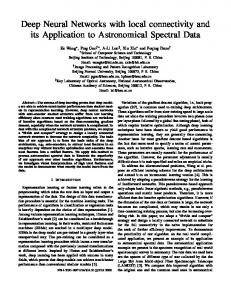
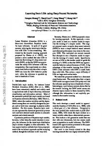
2 Two-dimensional Electrophoresis Images Two-dimensional electrophoresis images represent the difference between the isoelectric points and molecular weights of proteins [32, 33]. Figure 1 shows an overview of the process by which 2-DE images are produced, and Figure 2 illustrates examples of 2-DE images showing sepsis and non-sepsis. Such images are produced by first extracting and refining proteins from a sample. After that, the proteins are split off on the basis of the degree of isoelectric points and molecular weights. Therefore, the X-axis of 2-DE images represents the degree of molecular weights, Y-axis represents the degree of isoelectric points, and black regions represent the protein spots [28]. Normally, 2-DE images are analyzed for detection of a specific spot corresponding to a protein as a bio-marker, using computer assistance [5]. However, many diseases, such as sepsis, are multifactorial, which cause minute changes at many spots and unexpected spots in some cases. Therefore, when the polymerase chain reaction (PCR) method [3], which amplifies specific genes, is applied, we must guess the target genes, and testing of each gene must be carried out. If the number of biomarkers increases, the labor will also increase. On the other hand, if we directly use 2-DE images, this problem can be solved because we can consider the comprehensive changes of proteins at one time. From this situation, we try to use 2-DE images for diagnostic testing instead of using spot analysis. Figure 3 shows an overview of our system for detecting diseases by using 2-DE images. First, a doctor puts a sample of the blood of a patient on a micro-tip, then insert it into a device that can generate 2-DE images. Then, our system detects diseases and display the results to doctors. The main point with our system is to detect diseases, such as sepsis, with complex electrophoresis patterns of 2-DE
STUVWXY
� ������� � ��� �� ��� ����� �� ��� !"
#$%&'()*+ ,-./0123 45 678 9:;? @AB CDEFGHIJK LMNOPQR
Figure 1. Overview of production process of 2-DE images. After extracting and refining proteins from sample, proteins are split off by degree of isoelectric points and molecular weights (SDS-PAGE [32, 33]).
Z[\ ]^_`ab
cde fghijklmno Figure 2. Examples of 2-DE images. X- and Y-axes represent degrees of molecular weights and isoelectric points, respectively, and black regions represent protein spots.
images by using DNNs. It is a matter of course that current devices for generating 2-DE images are not suitable for this concept due to issues such as low-throughput ability and low reproducibility. A few groups [2, 17] have developed techniques to generate 2-DE images with high sensitivity, high throughput ability, and high reproducibility. However, even if they can solve these problems in generating 2-DE images, collecting 2-DE images produced from patients is difficult due to privacy and security concerns. This clearly indicates that the need for a classification method, such as ATDL, for a significantly small amount of training data is increasing.
3.2 Training Process
pqrst uvwxyz
3.2.1 Construction of Deep Neural Network for Source Task
{|}
~
Figure 3. Overview of our system for detecting diseases. We focused on classification step involving analysis using DNNs.
NOPQRS TUVWXY ��� ���
¸¹º
µ¶·
˜ i−1 + bi ). hi = s(W i h
ÜÝÞ ÷øù èéê ßàá úûü ôõö ëìí åæç òóñ âãä ýþÿ îïð � �
� åæçèéêëìíîï ðñòóô õö÷ø
���� ��� ���������� yz{|}~
Z[\]^_ `abcde fghi
()*
¦§¨ ©ª« ²³´ £¤¥ ¯°± ¡¢ ¬®
§¨©
ª«¬
"#$
ÅÆÇ ÈÉÊËÌ
%&' � !
jklm
¿ À Á
¤ ¥ ¦
®¯
»¼½¾ ¿ÀÁÂ ÇÈÉ ÃÄÅÆ
ÙÚÛ
It should be noted that layer i = 0 represents an input layer, that ˜0 = x ˜ s . The weight and bias are computed by minimizing a is, h de-noising reconstruction error [38]. At the output layer ((L + 1)-th layer), we apply a regression function f (.) and the cost function of Ds as follows,
nopq v w x rstu
� ���"� ¡¢£
ÊËÌÍ ÎÏÐÑ Ö×Ø ÒÓÔÕ
s
l({y s , xs }) =
N 1 X s ||y j − f (hL |xsj )||2 , s N j
(2)
°±²³ ´µ¶· ¼ ½ ¾ ¸¹º»
+,-./012 3456789
ÕÖ×ØÙÚ ÛÜÝÞßà áâãä
(1)
ùúûüýþÿ
ÍÎÏ ÐÑÒÓÔ
We first explain the SdA for constructing Ds . Let xs ∈ RDx denote a Dx dimensional source vector and W i and bi denote a weight matrix and bias vector of the i-th hidden layer (i = 1, 2, · · · , L), ˜ denote a corrupting vector drawn from corruption respectively. Let x process q(˜ x|x), and s(.) denote a sigmoid function. Then, the i-th hidden vector of Ds is as follows,
ÂÃÄ
where N s is the amount of source domain data, y sj is a label vector of xsj (yjs (k) = {0, 1}, k = 1, 2, · · · , Dy s ), Dy s is the dimension of y s , and f (hL |xsj ) = hL+1 = W L+1 hL + bL+1 .
(3)
The parameters of all layers are simultaneously fine-tuned using a stochastic gradient descent. In this article, we use {W i , bi |i = 1, 2, · · · , L + 1} as the initial parameters of Dt .
:;?@ABCD EFGHIJKLM
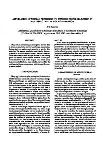
Figure 4. Outline of ATDL. (A): Training DNN for source task, (B): computing relation vectors of each target label, (C): tuning all parameters to transfer Ds to Dt .
3 All-Transfer Deep Learning
3.2.2 Computation of Relation Vectors Relation vectors represent the characteristics of the target labels in the Dy s dimensional feature space computed by the source domain knowledge, Ds . Let rl ∈ RDys denote the l-th relation vector (l = 1, 2, · · · , Dy t ), Dy t denote the number of target labels, and xtl ∈ RDx denote a target vector corresponding to the l-th target label. Then, rl is computed using the following equation.
3.1 Overview rl = arg max p(hL+1 |xtl ), hL+1 An outline of the ATDL training process is shown in Figure 4. First, ATDL trains a DNN, Ds , to solve the task of the source domain (Figure 4 (A)). In this study, we constructed Ds on the basis of stacked de-noising autoencoder (SdA) [12, 38]. Second, ATDL computes the output vectors of each target vector by inputting them into the DNN trained on the source domain data (Figure 4 (B)). It then computes the relation vectors of each target label. A relation vector denotes a vector representing the relationship between the source and target labels on the basis of the source domain knowledge, Ds , by using the output vectors. Finally, we fine-tune all parameters in such a way that the variance between the output and relation vectors is sufficiently small (Figure 4 (C)). By using the steps corresponding to Figures 4 (B) and (C), we can transfer Ds to the DNN for the target task Dt , regularizing all parameters including the output layer. This means that ATDL provides Dt , which can avoid the local-optimal solution caused by the randomness of the initial values.
(4)
where p(hL+1 |xtl ) is the probability distribution of hL+1 given xtl . We assume p(hL+1 |xtl ) obeys a Gaussian distribution. Therefore, rl is equal to the average vector of f (hL |xtl ). t
N (l) X 1 rl = t f (hL |xtl,j ), N (l) j
(5)
where xtl,j and N t (l) are the j-th target domain vector and amount of target domain data corresponding to the l-th target label, respectively. The k-th variable rl (k) means the strength of the relationship between the k-th source label and l-th target label. Therefore, by confirming the values of relation vectors, we can understand which labels of the source domain data are similar to those of the target domain data.
3.2.3 Fine-tuning After computing rl , we set r l as the l-th label vector of the target task, and all parameters including W L+1 and bL+1 are fine-tuned by minimizing the following main cost function using a stochastic gradient descent. It should be noted that this equation represents the variance of the target domain data. D
l({r, xt }) =
Table 1. CPU Memory GPU
Experimental environment. Intel (R) Core (TM) i7-4930K 64.0GB GeForce GTX 760
t
yt N (l) 1 X X ||r l − f (hL |xtl,j )||2 , Nt j
(6)
l
where N t = N t (1) + N t (2) + · · · + N t (Dy t ). By using this algorithm, we can have Dt regularizing all parameters by using Ds .
3.3 Classification Process In the classification process, Dt predicts the label ˆl of the test vector x on the basis of the following equation. ˆl = arg min(rl − f (hL |x))⊤ Σl (rl − f (hL |x)),
(7)
Figure 5. Examples of 2-DE images that differ in extraction and refining protocol of protein. Label number of source domain data is from 1 (top left) to 9 (bottom right) in order.
l
where Σl is a covariance matrix. It should be noted that classification performance does not improve if rˆl ≈ rˆl′ (ˆl 6= ˆl′ ). This means that the source domain/task is not suitable for transfer.
4 Experimental Results We conducted experiments on 2-DE image classification for determining if an individual suffers from sepsis. We compared the classification performance of five methods: non-transfer learning, simple semi-supervised learning (SSL), transfer learning by Agrawal et al. [1], that by Oquab et al. [29], and ATDL. The SSL is a method to construct a mixture model that computes hi using xs and xt and fine-tunes using only xt . In addition, this method is a special case of that by Weston et al. [40], which embeds the regularizer to the output layer, when the parameter to balance between the object function and regularizer is zero. Agrawal’s method removes the output layer of Ds and adds a new output layer. In addition to these two steps, Oquab’s method contains an additional adaptation layer to compensate for the different statistics of the source and target domain data. Then, Agrawal’s method fine-tunes all layers including the hidden layers [41], and Oquab’s method fine-tunes only the adaptation and output layers. In our study, we used a soft max function as the output layer for constructing Ds of the above transfer learning, SSL, and non-transfer learning methods. To investigate the difference in classification performance, we changed the source domain data and evaluated classification performance. We used 2-DE images that were given different labels from the target domain data of sepsis or non-sepsis, MNIST [25], and CIFAR-10 [21], as the source domain data. In addition, to investigate the generality of our method, we applied it to a convolutional neural network (CNN) [25] and a different task of open-image-data classifications. For open-image-data classifications, we investigated the effectiveness of our method for two open image data classifications. Finally, we investigated the correlation coefficients between the classification performance and Mahalanobis distance of rl .
4.1 Environment and Hyperparameter Settings We used the computer environment summarized in Table 1 and pylearn2 [15] to minimize (2) and (6). In this study, we set the learning rate to λ/(1.00004 × t), where t is the iteration. Momentum gradually increased from 0.5 to µ when t increased. We selected the initial learning rate λ from {1.0 × 10⁻³ , 5.0×10⁻³ , 1.0×10⁻² , 5.0×10⁻² }, final momentum µ from {0.7, 0.99}, and size of minibatches from {10, 100}.
4.2 Actual Sepsis-Data Classification Table 2. List of source 2-DE images. These images represent different extraction and refining protocols of proteins. # of source 2-DE images Type of protocol N s (1) = 25 Change amount of protein N s (2) = 4 Change concentration protocol N s (3) = 30 Unprocessed N s (4) = 49 Removal of only top-2 abundant proteins N s (5) = 11 Focus on top-2 abundant proteins N s (6) = 15 Focus on 14 abundant proteins N s (7) = 12 Plasma sample instead of serum N s (8) = 19 Removal of Sugar chain N s (9) = 15 Other protocols
For actual sepsis-data classification, we collected the following number of target 2-DE images N t = 98, sepsis data of N t (1) = 30 and non-sepsis data of N t (2) = 68. The size of the 2-DE images was 53 × 44 pixels (Dx = 2, 332), which was determined to save the information of the large spots. We evaluated classification performance on the basis of two-fold cross validation. As the source domain data, we first used 2-DE images with different labels from the target domain sepsis or non-sepsis data. These images were generated from patients which were diagnosed as being normal. The source task was to classify the differences between the extraction and refining protocols of proteins [39] shown in Table 2 and Figure 5. As shown in
Figure 6.
Example of relation vectors of actual sepsis-data classification.
this table, we set N s = 180 and Dy t = 9. On the other hand, the target 2-DE images were generated using serum and by removing 14 abundant proteins. These data were generated from actual patients at Juntendo University Hospital and were judged by infectious disease tests and SOFA/SIRS score [37]. This study was approved by the institutional review board, and written informed consent was obtained from patients.
4.2.1 Comparison with Conventional Methods Table 3. Classification performance of actual function of the number of hidden layers. PPV NPV PCA + logistic regression 0.875 0.805 Non-transfer (L=1) 0.725 0.983 Non-transfer (L=2) 0.718 0.967 Non-transfer (L=3) 0.644 0.981 Non-transfer (L=4) 0.644 0.981 SSL (L=1) 0.682 1 SSL (L=2) 0.644 0.981 SSL (L=3) 0.592 0.980 SSL (L=4) 0.558 0.978 Oquab et al. [29] (L=1) 0.732 1 Oquab et al. [29] (L=2) 0.771 0.952 Oquab et al. [29] (L=3) 0.702 0.934 Oquab et al. [29] (L=4) 0.658 0.947 Agrawal et al. [1] (L=1) 0.750 1 Agrawal et al. [1] (L=2) 0.744 0.983 Agrawal et al. [1] (L=3) 0.690 0.982 Agrawal et al. [1] (L=4) 0.667 1 ATDL (L=1) 0.844 0.955 ATDL (L=2) 0.871 0.955 ATDL (L=3) 0.875 0.970 ATDL (L=4) 0.958 0.905
sepsis-data classification as MCC 0.545 0.755 0.726 0.676 0.676 0.736 0.676 0.620 0.580 0.783 0.753 0.670 0.648 0.800 0.796 0.722 0.720 0.812 0.834 0.859 0.806
F1 0.609 0.829 0.811 0.773 0.773 0.811 0.773 0.734 0.707 0.845 0.831 0.776 0.761 0.857 0.841 0.806 0.8 0.871 0.885 0.903 0.852
ACC 0.816 0.878 0.867 0.827 0.827 0.857 0.827 0.786 0.755 0.888 0.888 0.847 0.827 0.898 0.888 0.857 0.847 0.918 0.929 0.939 0.918
We compared the classification performances, including that of ATDL, with respect to the changing number of hidden layers L = 1, 2, 3 and 4. We set the dimension of the 1st hidden layer to D1 = 188 by PCA using xs and xt (cumulative contribution of 188 features is over 99.5%), and D2 , D3 , and D4 were set to the same dimensions. Table 3 lists the classification accuracies (ACCs) of six methods including the baseline, PCA + logistic regression (used 188 features). It also lists the positive predictive values (PPVs), negative predictive values (NPVs), Matthews correlation coefficients (MCCs), and F1scores (F1s) as reference. It should be noted that PPV and NPV are
Figure 7. Example of relation vectors when source domain data are from CIFAR-10.
used in diagnostic tests, MCC is used for evaluating performance considering the unbalance-ness of N t (1) and N t (2), and F1 is the harmonic value computed by precision (=PPV) and recall. As shown in this table, classification accuracy improved by using transfer learning. In addition, the classification accuracy of ATDL (L = 3) outperformed those of the other transfer learning methods. For example, the classification accuracy of ATDL improved at least 4 percentage points compared to that of Agrawal’s method of L = 1. These results suggest that ATDL is effective for performing actual sepsis-data classification. Figure 6 shows an example of relation vectors of sepsis and nonsepsis (L = 3). The red bars represent the relation vector of sepsis, whereas the green bars represent that of non-sepsis. The numbers on the X-axis correspond to the source label indices listed in Table 2. As shown in this figure, the relation vectors of sepsis and non-sepsis differed. These results suggest that rl can represent the characteristics of the target label in the feature space computed by Ds .
4.2.2 Comparison of Various Source Tasks Table 4. Classification performance of actual sepsis-data classification for different source tasks.
Non-transfer (Di = 188) Non-transfer (Di = 500) Non-transfer (Di = 1, 000) CIFAR-10 (Di = 188) CIFAR-10 (Di = 500) CIFAR-10 (Di = 1, 000) MNIST (Di = 188) MNIST (Di = 500) MNIST (Di = 1, 000) 2-DE image (Di = 188) 2-DE image (Di = 500) 2-DE image (Di = 1, 000)
PPV 0.718 0.644 0.7 0.657 0.923 0.690 0.778 0.839 0.828 0.875 0.844 0.824
NPV 0.967 0.981 0.966 0.889 0.912 0.982 0.968 0.940 0.913 0.970 0.955 0.969
MCC 0.726 0.676 0.709 0.568 0.804 0.722 0.780 0.786 0.735 0.859 0.812 0.818
F1 0.811 0.773 0.8 0.708 0.857 0.806 0.849 0.852 0.813 0.903 0.871 0.875
ACC 0.867 0.827 0.857 0.806 0.918 0.857 0.898 0.908 0.888 0.939 0.918 0.918
We compared classification performance with respect to changing the source domain data, which were obtained from MNIST, CIFAR10, and 2-DE images. The number of images extracted from MNIST and CIFAR-10 were N s = 50, 000. The CIFAR-10 images were converted to gray-scale, and the MNIST and CIFAR-10 images were resized to Dx = 53 × 44 = 2, 332 to ensure they were aligned with the 2-DE images. In addition, we set L = 3 and D1 = D2 = D3 . We
Figure 8. Example of relation vectors when source domain data are from MNIST.
� �
�
�
������
��� � �� � � ����
Figure 9. CNN structure.
also evaluated classification performance with respect to changing the dimension of each hidden layer Di = 188, 500, and 1, 000. Table 4 lists the classification accuracies, and the PPVs, NPVs, MCCs, and F1s as reference. The classification accuracy based on the use of 2-DE images as the source domain data was higher than those obtained with MNIST and CIFAR-10, although the number of 2-DE images was smaller (N s = 180). Figure 7 shows an example of the relation vectors using CIFAR10 (Di = 500) and Figure 8 shows them using MNIST (Di = 500). Compared to Figure 6, the relation vector of sepsis was considerably closer to that of non-sepsis. These results show that information on the differences between the extraction and refining protocols of proteins is useful for classifying sepsis, rather than using CIFAR-10 and MNIST. Namely, if we collect the source domain data, we have to consider the relationship between the source and target domain data.
4.2.3 Applying ATDL to Convolutional Neural Network Table 5. Classification performance when ATDL was applied to CNN. PPV NPV MCC F1 ACC Non-transfer 0.717 0.966 0.726 0.812 0.867 ATDL 0.829 0.984 0.845 0.892 0.929
To investigate the effectiveness of our method regarding other DNNs, we applied it to a CNN and evaluated its classification performance by using 2-DE images as the source domain data. Figure 9 shows the structure of the CNN, which was determined on the basis of two-fold cross validation with respect to changing the hyperparameters shown in this figure. Table 5 lists the classification performances. The ATDL performed better than the non-transfer learning method and approximately equal to the SdA of ATDL (L = 3) shown in Table 3. Thus, these results suggest that ATDL is applicable to CNNs as well as SdAs. The CNN
Figure 10. Relation vectors when ATDL was applied to CNN. Numbers on X-axis correspond to source label indices.
is widely used in image recognition and achieves high classification accuracy on several standard data [19, 23, 24]. Therefore, we consider that ATDL is possible to be applied to various image recognition problems. Figure 10 shows the relation vectors. Sepsis had a relationship to the 4th source label (removal of only top-2 abundant proteins), which is the same as in Figure 6. This result suggests that there are biological relationships between them. In the future, we plan to examine this result from a biological point of view.
4.3 Open-Image Data Experiment Table 6. Accuracy of automobile and pedestrian crossing. # of target images N t 400 1,500 Non-transfer 0.724 0.753 SSL 0.750 0.789 Oquab et al. [29] 0.763 0.782 Agrawal et al. [1] 0.753 0.781 ATDL 0.789 0.797
Table 7. Accuracy of MNIST. # of target images N t 1,000 5,000 Non-transfer 0.854 0.926 SSL 0.844 0.928 Oquab et al. [29] 0.773 0.875 Agrawal et al. [1] 0.844 0.923 ATDL 0.887 0.928
10,000 0.945 0.951 0.887 0.951 0.932
To investigate the generalization of our method, we first applied our method to two open image data classifications: (1) CIFAR10 [21] as the source domain and images of an automobile and pedestrian crossing from ImageNet [22] as the target domain, and (2) SVHN [27] as the source domain and MNIST [25] as the target domain. Task (1) is an example in which the source/target domain data consist of color images, and (2) is an example of multiclass classification. For task (1), we constructed Ds on the basis of the SdA and set L = 3, Dy s = 10, Di = 1, 000 (i = 1, 2, 3), and N s = 50, 000. As the target test data, we used 750 images of automobile and 750 images of pedestrian crossing. For task (2), we also constructed Ds on the basis of the SdA and set L = 3, Dy s = 10, Di = 100 (i =
Figure 11.
Example of relation vectors of task (1).
89: 567
F
G
234
H
I
/01 [ ,-.
Figure 13. Relationship between Mahalanobis distance and classification performance. Blue lines represent classification performance of non-transfer learning method.
)*+ &'( % !#$
;
? @ A B JKLMNO PQRST UVWXYZ
C
DE
Figure 12. Example of relation vectors of task (2) (N t = 1, 000).
Table 8. Correlation coefficient R and p-value of each classification performance. PPV NPV MCC F1 ACC R 0.627 0.521 0.663 0.657 0.665 p-value < 0.01 < 0.01 < 0.01 < 0.01 < 0.01
1, 2, 3), N s = 73, 257, and SVHN images were converted to grayscale. As the target test data, we used 10, 000 images from MNIST. Test images of task (1) and (2) were not included in the training target domain data. Table 6 and 7 list the classification accuracies of the five methods for different amounts of target domain data. It should be noted that we could not conduct actual sepsis-data classification in this experiment because collecting sepsis data is difficult. As shown in these tables, our method outperformed other methods when N t = 400, 1, 500 for task (1) and N t = 1, 000 for task (2). These results suggest that our method is effective when the amount of target domain data is significantly small. Figure 11 and 12 show examples of the relation vectors of each task. As shown in these figures, the target automobile showed a relationship with the source automobile (2nd source label) and source truck (10th source label). In addition, the highest relation of the character “6” of MNIST was the character “6” of SVHN. On the other hand, the relation vectors of the target automobile/pedestrian crossing differed. These results suggest that r l enabled the representation of the target label characteristics in the feature space computed by Ds , the same as 2-DE images.
transfer. Let M denote the number of source domain sub-groups, Nas (a = 1, 2, · · · , M ) denote the amount of a-th source domain sub-group data, and X a = {y sb , xsb |b = 1, 2, · · · , Nas } denote the a-th source domain sub-group data sampled from all source domain data X. We constructed Dsa by using X a and computed the Mahalanobis distance dm (a) of r l by inputting the a-th DNN Dsa . Then, we finetuned to transfer from Dsa to Dt . We used MNIST as X and set M = 100 and Nas = 5, 000 (a = 1, 2, · · · , M ). Sub-groups were randomly selected from X, and Dsa was constructed on the basis of the SdA. The target task was sepsis-data classification, and we set L = 1, D1 = 188, and N t = 49 (N t (1) = 15, N t (2) = 34). As the target test data, we used 15 images of sepsis and 34 images of non-sepsis. It should be noted that all hyperparameters were fixed. To evaluate the relationship between dm (a) and classification performance t(a), we computed the correlation coefficient R as follows.
4.4 Correlation of Performance and Distance As described above, the classification performance of ATDL depends on the distance of rl . In this subsection, we discuss the investigation of the correlation between classification performance and Mahalanobis distance dm . If they correlate, ATDL can be used to select Ds before the fine-tuning process and reduce the risk of negative
PM (dm (a) − d¯m )(t(a) − t¯) R = qP a , M ¯ 2 PM (t(a) − t¯)2 a (dm (a) − dm ) a
(8)
where d¯m and t¯ are the averages of dm and t. Figure 13 shows dm (a) and the corresponding classification performances, and Table 8 lists the correlation coefficients and p-values. The blue lines in Figure 13 represent the performance of non-transfer learning. The Mahalanobis distance and classification performances correlated, suggesting that higher classification performance than that of non-transfer learning
is possible by using Dsa with large dm (a). This means that we can select Dsa effectively before the fine-tuning process.
5 Conclusion We proposed ATDL, a novel transfer learning method for DNNs, for a significantly small amount of training data. It computes the relation vectors that represent the characteristics of target labels by the source domain knowledge. By using the relation vectors, ATDL enables the transfer of all knowledge of DNNs including the output layer. We applied ATDL to actual sepsis-data classification. The experimental results showed that ATDL outperformed other methods. We also investigated the generality of ATDL with respect to changing the DNN model and target task, and compared the classification performance with respect to changing the source domain data. From the results, we argue that our method is applicable to other tasks, especially when the amount of target domain data was significantly small, and classification performance improves when we use the source domain data that are similar to the target domain data. Furthermore, we showed the possibility of selecting an effective DNN before the fine-tuning process. To the best of our knowledge, this work involved the first trial in which 2-DE images were analyzed using the classification approach, which resulted in over 90% accuracy. Thus, this article will be influential not only in machine learning, but also medical and biological fields. In the future, we will collect source domain 2-DE images that can be uploaded easily, apply ATDL to a deeper network, predict classification performance more accurate, and analyze the relation vectors from a biological point of view.
6 Acknowledgments We would like to acknowledge Dr. Iba, Professor of Juntendo University School of Medicine, for his help in collecting samples to generate 2-DE images.
REFERENCES [1] Pulkit Agrawal, Ross Girshick, and Jitendra Malik, ‘Analyzing the performance of multilayer neural networks for object recognition’, in Proceedings of the European Conference on Computer Vision, 329–344, (2014). [2] Stephen Barnes, Helen Kim, and Victor M Darley-Usmar, ‘High throughput two-dimensional blue-native electrophoresis: a tool for functional proteomics of mitochondria and signaling complexes’, Proteomics, 2, 969–977, (2002). [3] John MS Bartlett and David Stirling, ‘A short history of the polymerase chain reaction’, PCR protocols, 3–6, (2003). [4] Yoshua Bengio, ‘Learning deep architectures for AI’, Foundations and trends in Machine Learning, 2(1), 1–127, (2009). [5] Matthias Berth, Frank Michael Moser, Markus Kolbe, and J¨org Bernhardt, ‘The state of the art in the analysis of two-dimensional gel electrophoresis images’, Applied microbiology and biotechnology, 76(6), 1223–1243, (2007). [6] R Phillip Dellinger, Mitchell M Levy, Andrew Rhodes, Djillali Annane, Herwig Gerlach, Steven M Opal, Jonathan E Sevransky, Charles L Sprung, Ivor S Douglas, Roman Jaeschke, et al., ‘Surviving sepsis campaign: international guidelines for management of severe sepsis and septic shock, 2012’, Intensive care medicine, 39(2), 165–228, (2013). [7] Jia Deng, Wei Dong, Richard Socher, Li-Jia Li, Kai Li, and Li Fei-Fei, ‘Imagenet: A large-scale hierarchical image database’, in Proceedings of the IEEE Conference on Computer Vision and Pattern Recognition, pp. 248–255, (2009).
[8] Chuong Do and Andrew Y Ng, ‘Transfer learning for text classification’, in Proceedings of the Advances in Neural Information Processing Systems, pp. 299–306, (2005). [9] Viktor Y Dombrovskiy, Andrew A Martin, Jagadeeshan Sunderram, and Harold L Paz, ‘Rapid increase in hospitalization and mortality rates for severe sepsis in the united states: A trend analysis from 1993 to 2003’, Critical care medicine, 35(5), 1244–1250, (2007). [10] Jeff Donahue, Yangqing Jia, Oriol Vinyals, Judy Hoffman, Ning Zhang, Eric Tzeng, and Trevor Darrell, ‘Decaf: A deep convolutional activation feature for generic visual recognition’, in Proceedings of the International Conference on Machine Learning, pp. 647–655, (2014). [11] Chao Dong, Chen Change Loy, Kaiming He, and Xiaoou Tang, ‘Learning a deep convolutional network for image super-resolution’, in Proceedings of the European Conference on Computer Vision, 184–199, Springer, (2014). [12] Dumitru Erhan, Yoshua Bengio, Aaron Courville, Pierre-Antoine Manzagol, Pascal Vincent, and Samy Bengio, ‘Why does unsupervised pretraining help deep learning?’, The Journal of Machine Learning Research, 11, 625–660, (2010). [13] Mark Everingham, Luc Van Gool, Christopher KI Williams, John Winn, and Andrew Zisserman, ‘The pascal visual object classes (VOC) challenge’, International journal of computer vision, 88(2), 303–338, (2010). [14] Yaroslav Ganin and Victor Lempitsky, ‘Unsupervised domain adaptation by backpropagation’, in ICML, pp. 1180–1189, (2015). [15] Ian J. Goodfellow, David Warde-Farley, Pascal Lamblin, Vincent Dumoulin, Mehdi Mirza, Razvan Pascanu, James Bergstra, Fr´ed´eric Bastien, and Yoshua Bengio, ‘Pylearn2: a machine learning research library’, arXiv preprint arXiv:1308.4214, (2013). [16] Geoffrey Hinton, Oriol Vinyals, and Jeff Dean, ‘Distilling the knowledge in a neural network’, in Proceedings of the Deep Learning and Representation Learning Workshop, (2014). [17] Atsunori Hiratsuka, Hideki Kinoshita, Yuji Maruo, Katsuyoshi Takahashi, Satonari Akutsu, Chie Hayashida, Koji Sakairi, Keisuke Usui, Kisho Shiseki, Hajime Inamochi, et al., ‘Fully automated twodimensional electrophoresis system for high-throughput protein analysis’, Analytical chemistry, 79(15), 5730–5739, (2007). [18] Junlin Hu, Jiwen Lu, and Yap-Peng Tan, ‘Deep transfer metric learning’, in Proceedings of the IEEE Conference on Computer Vision and Pattern Recognition, pp. 325–333, (2015). [19] Yangqing Jia, Evan Shelhamer, Jeff Donahue, Sergey Karayev, Jonathan Long, Ross Girshick, Sergio Guadarrama, and Trevor Darrell, ‘Caffe: Convolutional architecture for fast feature embedding’, in Proceedings of the ACM International Conference on Multimedia, pp. 675–678, (2014). [20] Jing Jiang and ChengXiang Zhai, ‘Instance weighting for domain adaptation in nlp’, in Proceedings of the Annual Meeting of the Association for Computational Linguistics, pp. 264–271, (2007). [21] Alex Krizhevsky and Geoffrey Hinton. Learning multiple layers of features from tiny images. master’s thesis, university of tronto, 2009. [22] Alex Krizhevsky, Ilya Sutskever, and Geoffrey E Hinton, ‘Imagenet classification with deep convolutional neural networks’, in Proceedings of the Advances in neural information processing systems, pp. 1097– 1105, (2012). [23] Alex Krizhevsky, Ilya Sutskever, and Geoffrey E Hinton, ‘Imagenet classification with deep convolutional neural networks’, in NIPS, volume 1, pp. 1–9, (2012). [24] Quoc V Le, ‘Building high-level features using large scale unsupervised learning’, in Proceedings of the IEEE International Conference on Acoustics, Speech and Signal Processing, pp. 8595–8598, (2013). [25] Yann LeCun, L´eon Bottou, Yoshua Bengio, and Patrick Haffner, ‘Gradient-based learning applied to document recognition’, in Proceedings of the IEEE, volume 86, pp. 2278–2324, (1998). [26] Mingsheng Long, Yue Cao, Jianmin Wang, and Michael Jordan, ‘Learning transferable features with deep adaptation networks’, in ICML, pp. 97–105, (2015). [27] Yuval Netzer, Tao Wang, Adam Coates, Alessandro Bissacco, Bo Wu, and Andrew Y Ng, ‘Reading digits in natural images with unsupervised feature learning’, In NIPS workshop on deep learning and unsupervised feature learning, 1–9, (2011). [28] Patrick H O’Farrell, ‘High resolution two-dimensional electrophoresis of proteins.’, Journal of biological chemistry, 250(10), 4007–4021, (1975). [29] Maxime Oquab, Leon Bottou, Ivan Laptev, and Josef Sivic, ‘Learning
[30] [31] [32] [33] [34]
[35] [36] [37]
[38]
[39] [40] [41] [42]
[43]
and transferring mid-level image representations using convolutional neural networks’, in Proceedings of IEEE Conference on Computer Vision and Pattern Recognition, pp. 1717–1724, (2014). Sinno Jialin Pan, Ivor W Tsang, James T Kwok, and Qiang Yang, ‘Domain adaptation via transfer component analysis’, IEEE Transactions on Neural Networks, 22(2), 199–210, (2011). Sinno Jialin Pan and Qiang Yang, ‘A survey on transfer learning’, IEEE Transactions on Knowledge and Data Engineering, 22(10), 1345–1359, (2010). Thierry Rabilloud, Mireille Chevallet, Sylvie Luche, and C´ecile Lelong, ‘Two-dimensional gel electrophoresis in proteomics: past, present and future’, Journal of proteomics, 73(11), 2064–2077, (2010). Thierry Rabilloud and C´ecile Lelong, ‘Two-dimensional gel electrophoresis in proteomics: a tutorial’, Journal of proteomics, 74(10), 1829–1841, (2011). Michael T Rosenstein, Zvika Marx, Leslie Pack Kaelbling, and Thomas G Dietterich, ‘To transfer or not to transfer’, in Proceedings of the NIPS’05 Workshop on Inductive Transfer: 10 Years Later, volume 2, pp. 7–10, (2005). Kate Saenko, Brian Kulis, Mario Fritz, and Trevor Darrell, ‘Adapting visual category models to new domains’, in Proceedings of the European Conference on Computer Vision, 213–226, (2010). Yoshihide Sawada, Yoshikuni Sato, Toru Nakada, Kei Ujimoto, and Nobuhiro Hayashi, ‘All-transfer learning for deep neural networks and its application to sepsis classification’, in ECAI, pp. 1586–1587, (2016). Mervyn Singer, Clifford S Deutschman, Christopher Warren Seymour, Manu Shankar-Hari, Djillali Annane, Michael Bauer, Rinaldo Bellomo, Gordon R Bernard, Jean-Daniel Chiche, Craig M Coopersmith, et al., ‘The third international consensus definitions for sepsis and septic shock (sepsis-3)’, Jama, 315(8), 801–810, (2016). Pascal Vincent, Hugo Larochelle, Isabelle Lajoie, Yoshua Bengio, and Pierre-Antoine Manzagol, ‘Stacked denoising autoencoders: Learning useful representations in a deep network with a local denoising criterion’, The Journal of Machine Learning Research, 11, 3371–3408, (2010). John M Walker, The proteomics protocols handbook, Springer, 2005. Jason Weston, Fr´ed´eric Ratle, Hossein Mobahi, and Ronan Collobert, ‘Deep learning via semi-supervised embedding’, in Neural Networks: Tricks of the Trade, 639–655, Springer, (2012). Jason Yosinski, Jeff Clune, Yoshua Bengio, and Hod Lipson, ‘How transferable are features in deep neural networks?’, in Advances in Neural Information Processing Systems, pp. 3320–3328, (2014). Bolei Zhou, Agata Lapedriza, Jianxiong Xiao, Antonio Torralba, and Aude Oliva, ‘Learning deep features for scene recognition using places database’, in Proceedings of the 27th Advances in Neural Information Processing Systems, pp. 487–495, (2014). Fuzhen Zhuang, Xiaohu Cheng, Ping Luo, Sinno Jialin Pan, and Qing He, ‘Supervised representation learning: transfer learning with deep autoencoders’, in Proceedings of the International Conference on Artificial Intelligence, pp. 4119–4125, (2015).