[2] Soderstrom Torsten, Stoica Petre: System. Identification. Warszawa 1997. PWN translated by. Banasiak J. [3] Emanuel Parzen: On Estimation of a Probability.
A robust linear-quadratic moving averaging area controller for strongly nonlinear systems This paper presents a new method of designing LQR controllers for a class of strongly nonlinear systems. Strongly nonlinear parabolic equations [9] have been studied by Browder [7] and by Lions [8] using the theory of monotone operators defined on a reflexive separable Banach space. An algorithm is presented that is based on a new approach to the linearization of the Bounded-Input Bounded-Output (b.i.b.o.) of nonlinear systems. The use of the classic LQR controller in real systems is not always possible in view of the non-linearity of the system, the astatic of the state matrix, and the limited precision of the numerical calculation of coefficients. So, the proposed approach for designing LQR controllers uses by averaging the linear-moving infinite impulse response (IIR) filters in the observed area.
Fig. 5. The structure of the closed loop LQR control with linearization feedback.
A linearizable observer is defined as a linear combination by the AutoRegressive–Moving-Average model with eXogenous inputs (ARMAX), Output-Error model infinite impulse response moving average (IIR-MA) estimator (19). 𝑦̃(𝑖) = 𝑧 −𝑘
Fig. 4. Nonlinear system modeled by the Wiener Hammerstein system.
We want to optimally approximate the non-linear system for the representation input reference signal to output by the linear system. Class of linear systems marked by a 𝑊, which we will solve for the optimal approximation is represented by convolution (15)[1]. ∞
𝑦𝐿 (𝑡) = (𝑊(𝑢0 )) ≔ ∫−∞ 𝜔(𝑡)𝑢0 (𝑡 − 𝜏)𝑑𝜏 ,
𝑥̇ = 𝑓𝑢1 + 𝑔𝑢2 , [𝑓, 𝑔] = ∞
𝜕𝑔 𝜕𝑞
𝑓−
𝜕𝑓 𝜕𝑞
∫0 |𝜔(𝜏)|𝑑𝜏 < ∞,
(16)
𝑔,
(17) (18)
Equation (15) ensures that limited entry u(·) linear system 𝑊 will generate a limited output.
+
𝐶(𝑧 −1 ) 𝜀(𝑖), 𝐴(𝑧 −1 )
(19)
For this reason, we can perform the linearization of the moving average area. For the non-zero initial condition: 𝐺̂ (𝑧) = 𝐺̃ (𝑧)ℎ(𝑧),
(20)
where 𝑢̂(𝑡) = 𝑓(ℎ(𝑧), 𝑢̃(𝑧)) obtain the assumption (21)
(15)
Consider a system which fulfill the assumptions [1]: The stability of the system with limited input and output, Bounded-Input Bounded-Output (b.i.b.o.). For a given 𝑏, there is 𝑚0 (𝑏) such that |𝑢(𝑡)| < 𝑏 ⇒ |𝑁𝑢(𝑡)| < 𝑚0 (𝑏) for all 𝑡 ∈ [0, ∞[. We assume limitation non-linearity, bounded-input to the nonlinear system generates limited signal an output. Cause stable approximators. Class of linear systems which will approximate the non-linear system assumes that the linear system to meet the principle of causality and the system is stable with limited input and output 𝜔(𝑡) ≡ 0 ∀ 𝑡 < 0. Non-linear system is controllable, the Lie matrix (17) has full rank.
𝐵(𝑧 −1 ) 𝑢̃(𝑖) 𝐴(𝑧 −1 )
𝑙𝑖𝑚𝑖𝑛𝑓𝑡→∞ |𝑢(𝑡) − 𝑢̂(𝑡)| → 𝜗𝑚𝑖𝑛 ,
(21)
𝜃̃𝑖 = [Φ𝑖 𝑇 Φ𝑖 ]−1 Φ𝑖 𝑇 𝑌𝑖 , ̃𝑖 (𝑧)] , 𝑌̃𝑖 = 𝑍 −1 [𝐺̃𝑖 (𝑧)𝑈
(22)
𝜃̂ = 𝑎𝑟𝑔 min𝜃̃𝑖 (𝑌𝑖 −
(24)
𝑌̃𝑖 )2 ,
(23)
system equations obtained 𝑥̇ = 𝐴𝑥 + 𝐵𝑢 + 𝜈, 𝑦 = 𝐶 𝑇 𝑥 + 𝑤,
(25) (26)
for linearized Wiener Hammerstein system representation obtained 𝑥̃̇ = 𝐴̂𝑥̃ + 𝐵̂𝑢̂, 𝑦̃ = 𝐶̂ 𝑇 𝑥̃,
(27) (28)
where 𝑥̃ ∈ ℝ𝑛 , 𝑢̂ ∈ ℝ𝑚 , 𝑦̃ ∈ ℝ𝑟 the controllable form of state equations obtained (29) −𝑎̂𝑛−1 −𝑎̂𝑛−2 ⋯ −𝑎̂1 1 0 1 ⋯ ⋯ ⋯ ] , 𝐵̂ = [ ], ⋯ ⋯ 1 ⋯ ⋯ 0 ⋯ ⋯ 1 0 𝐶̂ = [𝑐𝑛 𝑐𝑛−1 ⋯ 𝑐1 ], 𝐷 = 0
𝐴̂ = [
(29)
Luenberger state observer (30) 𝑥̂̃̇ = 𝐴̂𝑥̂̃ + 𝐵̂𝑢̂ + 𝐿(𝑦 − 𝐶̂ 𝑥̂̃ ), 𝑒𝐿 = 𝑥̂̃ − 𝑥 ,
(30)
𝑒̇𝐿 = (𝐴̂ − 𝐿𝐶̂ )𝑒𝐿 ,
(32)
(31)
For the linearized system, the controllability condition in the continuous-time defined cost function on an infinite horizon (31). ∞ 𝐽 = ∫0 (𝑥̂̃ 𝑇 𝑄𝑥̂̃ + 𝑢̂𝑇 𝑅𝑢̂)𝑑𝑡 , (33)
𝐴̂𝑇 𝑃 + 𝑃𝐴̂ − 𝑃𝐵̂𝑅−1 𝐵̂𝑇 𝑃 + 𝑄 = 0,
(34)
where 𝑄 ≥ 0, 𝑅 ≥ 0, 𝑃 ≥ 0 are symmetric, positive (semi-) definite matrices. Solving equation of the cost function gives us the control law for linearization feedback. 𝐾 = 𝑅−1 𝐵̂𝑇 𝑃, 𝑢 = −𝐾𝑥̂̃ ,
(35) (36)
The rights of the control operator can be entered as operators preferences of optimality to the trajectories of the state variables or the control value.
Fig. 7. Tracking of trajectory by nonlinear system (37)[6].
Conclusion
1. Example Example task of tracking a nonlinear system described in [6]. Given is nonlinear system, example [6](Fig. 20. Eq. (12)) described by the equation 𝑥⃛ + 𝑎𝑥̈ + 𝑥̇ = 𝑠𝑔𝑛(𝑥) − 𝑥, 𝑎 = 5,
(37)
linearized observer (9) for discrete points of samples 𝑘 = 141, 𝑢̂(𝑛 − 𝑘, 𝑛) ∈ [−1,1], 𝑦̃(𝑛 − 𝑘, 𝑛) ∈ [−3𝑒4, 2.5𝑒4), 𝑛 ∈ ℕ[1, ∞), 𝑘 ∈ ℕ on the fixed-step Δ𝑡 = 0.01, obtain 0.000002620100438 −0.000002079322727 −0.499998379648706 𝐴̂ = [ ] 1 0 0 0 1 0 1 𝐵̂ = [0] 0 𝐶̂ = [0.000004149913067 0.002500530184676 0.499999621780322]
The control matrix for linearized feedback obtain 𝐾 = [1.684627167749903 1.418979933264466 0.097614433718026]
Fig. 6. Stabilization of a nonlinear system (37)[6].
The proposed filtration algorithm has the properties of self-correction learning and self-tuning. The identification algorithm is fast and robust. In relation to available computing resources the algorithm may classify for fast algorithms. This allows to use the identification algorithm for system identification in space process and motion control. Fast, robust online identification at any time in the window horizon opens up good conditions and possibilities for the design of LQR controllers, model predictive controllers, and adaptive systems. The proposed control algorithm is computationally stable, gives good results in the control of strongly non-linear systems. All algorithms are easy to numerical implement in computer control systems.
References [1] S. Sastry: Nonlinear Systems. Analysis, Stability, and Control. 1999 Springer Science+Business Media New York, LLC. Interdisciplinary Applied Mathematics, Volume 10. [2] Soderstrom Torsten, Stoica Petre: System Identification. Warszawa 1997. PWN translated by Banasiak J. [3] Emanuel Parzen: On Estimation of a Probability Density Function and Mode. Annals of Mathematical Statistics, Volume 33, Issue 3 (Sep., 1962), 1065-1076. [4] Hassan K. Khail: Nonlinear Control. Global Edition. 2015. Pearson Education Limited Edinburgh Gate Harlow Essex CM20 2JE. England. J. C. Sprott: Algebraically Simple Chaotic Flows. International Journal Of Chaos Theory And Applications Volume 5 (2000), No. 2. [5] S. H. Żak.: Systems and Control. School of Electrical and Computer Engineering Purdue University. New York Oxford Oxford University Press 2003. [6] J. C. Sprott., Stefan J. Linz.: Algebraically Simple Chaotic Flows, attractor for the chaotic system example. International Journal of Chaos Theory and Applications, Volume 5 (2000), No. 2. [7] F. E. Brooder.: Strongly nonlinear parabolic boundaryvalue problems, Amer. J. Math. 86 (1964), 339-357. [8] J. L. Lions.: Sur certaines equations paraboliques nonlineaires, Bull. Sm. Math. Frunce 93 (1965), 155-175. [9] Bui An Ton.: On Strongly Nonlinear Parabolic Equations. Journal of functional analysis 7, 147-155 (1971)