composites, with results that would improve further with additional training data. ... adaptive SHM methodology to accommodate perturbations in structural ...
An Adaptive Pattern Recognition Methodology for Damage Classification in Composite Laminates Seth S. Kessler and Pramila Agrawal Metis Design Corporation
ASC-2007
ABSTRACT1 Composites present additional challenges for inspection due to their anisotropy, the conductivity of the fibers, the insulating properties of the matrix, and the fact that damage often occurs beneath the visible surface. This paper addresses the characterization of damage within composite materials, specifically for structural health monitoring (SHM). The presented research utilized Lamb wave testing coupled with pattern recognition methods, with the goal of providing the presence, type, and severity of damage with a high degree of confidence. An adaptive methodology is also presented to accommodate changes in structural response that are not attributable to damage, such as ageing, maintenance and repair. The results have shown that PR methods can be used to successfully characterize damage in composites, with results that would improve further with additional training data. INTRODUCTION Structural Health Monitoring (SHM) implies the incorporation of a nondestructive evaluation system into a structure to provide continuous remote monitoring for damage, with the goal of improved safety and reduced life-cycle costs. Lamb wave methods have been proven a reliable technique to collect valuable information about the state of damage within a structure, and several investigators have successfully used Lamb waves to determine the location of damage within composite plates [1-5]. Traditional algorithms are susceptible to rising false positive rates over time due to ageing materials, scheduled maintenance procedures and new structural repairs. In addition, slight differences between aircraft in a fleet, such as those due to sensor placement, bondline preparation and manufacturing tolerances, could have a significant adverse effect on accuracy as Seth S. Kessler, Metis Design Corporation, 10 Canal Park, Cambridge, MA 02141 Pramila Agrawal, Metis Design Corporation, 10 Canal Park, Cambridge, MA 02141
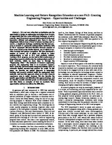
well. Ideally, these issues could be overcome by revising algorithms, manually updating threshold levels or re-training software for individual aircrafts continuously over time, however this solution is logistically impractical as well as extremely time consuming, potentially negating the original benefits of deploying an SHM system. Furthermore, tailored changes to algorithms could invalidate or at lease complicate the certification of an SHM system. This paper discusses an adaptive SHM methodology to accommodate perturbations in structural response not attributable to damage, while maintaining or accounting for algorithm accuracy. The objective of this work was to develop an analytical methodology that uses Lamb waves to characterize damage states in composite materials, with the goal of predicting the presence, type and severity with a high degree of confidence. DEFINING DAMAGE IN COMPOSITE MATERIALS There are several challenges in detecting damage in composite materials. Ideally, a simple pristine or damaged categorization would reside at the top level, however taking a micromechanics view, composite is fabricated with damage. Those microscopic flaws grow slowly over time, and can be greatly accelerated by events such as overloads or impacts, until a critical damage size is achieved [6]. Therefore the concept of a damage threshold must be introduced. At some level of detectable flaw size, the structure must be labeled as “damaged”. In composite materials, damage modes of interest include delamination, matrix microcracks, fiber fracture, swelling or brooming, and disbonding from secondary structure. Using one or two features to distinguish between these modes may not be feasible, as they may not be linearly separable. While it may be possible to differentiate between damage and no damage, or between 2 discrete damage modes with limited features, it is not possible to separate the entire mode space for composite materials with only 2 features to classify. It becomes necessary to extract several feature sets to allow multi-dimensional classification of damage modes. Using a very large set of features, however, may lead to the problems of redundancy and computational inefficiencies. In that case, feature–reduction techniques need to be employed to reduce dimensionality. Finally appropriate pattern recognition method must be chosen and trained using this feature data to successfully characterize the damage. TRADITIONAL METHODOLOGY FOR SHM ALGORITHMS The Standard Training Flowchart, seen in Figure 1, indicates the steps necessary to calibrate a generic SHM algorithm, essentially characterizing the definitions for various states. Generally, training input consisting of data linked to complementary damage state is iterated through a series of signal processing steps to establish the training output parameters to be locked and used for testing. A separate set of validation input is also utilized to establish state confidence levels. The Standard Testing Flowchart, seen in Figure 2, is executed to determine the present state of a structure given the training output parameters. Beyond the acquired test data, only an undamaged baseline from the test structure is required to apply the previously developed algorithms and calculate prediction accuracy.
Training Input Training Output
Signal Condition
Training Baseline
Feature Extraction Feature Selection Feature Reduction Pattern Recognition
Feature Parameters
Algorithm Development
Recognition Dictionary
Validation Input
Localization Algorithm
Confusion Matrix Figure 1: Training Flowchart used to derive optimized damage characterization algorithm Training Flowchart Input Training Input – voltage versus time data linked to damage presence, type, size and location info Validation Input – separate set identical to training input used to validate generated algorithms Iterative Functional Blockset Signal Condition – signal processing tools to remove unwanted artifacts, filter and de-noise data Feature Extraction – extracts quantifiable features from time, frequency and energy domains to characterize signal (max amplitude, arrival time, peak frequency, etc.) Feature Selection – most discriminative features are down-selected, such as those that are most consistent within a particular class and most variable between classes Feature Reduction – techniques to reduce the dimensionality of the selected features Pattern Recognition – models used to associate test data with a pre-trained classification Algorithm Development – equations to determine distance to damage based on time of flight Training Output Feature Parameters – designates selected features to extract and appropriate reductions Training Baseline – defines statistical average for all undamaged structure Recognition Dictionary – defines pattern recognition state machines Localization Algorithm – compiled algorithm to determine distance to damage Confusion Matrix – table of statistical accuracies of algorithms applied to validation data
Data Acquisition Training Output
Signal Condition
Testing Baseline
Feature Extraction Feature Reduction Pattern Recognition Presence, Type & Size
Localization Algorithm Confusion Matrix
Damage Location
Confidence Levels Figure 2: Testing Flowchart Testing Flowchart Input Data Acquisition – raw voltage versus time data is acquired from sensors Testing Baseline – undamaged baseline signal taken from test structure prior to testing Training Output – parameters generated by the Training Flowchart govern the testing algorithms Functional Blockset Signal Condition – filtering and denoising pre-set in Training Flowchart Feature Extraction – extraction of selected features optimized in Training Flowchart Feature Reduction – reduction of feature dimensionality pre-set by Training Flowchart Pattern Recognition – using the recognition dictionary from the Training Flowchart Localization Algorithm – using the algorithms generated in the Training Flowchart Confusion Matrix – matrix generated using validation input is used to assign confidence levels Testing Output Presence of Damage – pattern recognition determines presence of damage above threshold value Type of Damage – pattern recognition determines type of damage or “unknown” class Size of Damage – pattern recognition determines severity of damage within pre-set ranges Location of Damage – time of flight algorithm determines approximate location of damage Confidence Levels – validated confusion matrix yields confidence levels for each damage state
Signal Conditioning Signal conditioning is employed to de-noise the acquired signal from unwanted frequency content. Noise can generally be described by 2 categories: coherent and incoherent. Incoherent noise is typically referred to as “white noise,” and can be easily removed through averaging. The source of coherent noise is often more challenging to discover, however can originate from a multitude of EMI sources. While more challenging to identify, coherent noise is also relatively easily extracted within the frequency domain, as long as close attention is paid to not disturbing the phase of the signal. Once the data has been conditioned, another important component of the pre-processing stage is the removal of unwanted artifacts, which could include boundary conditions as well as pre-existing conditions. This is achieved by a variety of techniques in the time, frequency and/or wavelet domains, with the simple goal of eliminating pre-existing characteristics of the signal, typically by using baseline measurements. Feature Extraction To perform pattern classification, a set of discriminative features needs to be obtained from the data. Within the Lamb wave results investigated during the present research, there are 3 main easily identifiable domains from which these features can be extracted: Time, Frequency and Energy. The Time Domain features are amongst the most commonly used in analysis, and include “time of flight” (TOF) and time position of the maximum and subsequent secondary peaks. These features can be observed from the raw data itself with little processing. Frequency Domain features include the maximum value of power spectral density (PSD), general distribution of power at various frequencies, shift in frequency response from baseline, as well as the actual frequency and phase at this value. Frequency features can be extracted by using both Fourier transforms as well as Wavelet decomposition, where the effectiveness depends on the shape of the excitation signal. Finally, the Energy Domain features include the mean and standard deviation for the original signal amplitude as well as the 1st and 2nd differences of the signal amplitude. Other features of this domain include the total integrated signal energy, the maximum peak amplitude and the amplitude of other representative envelope locations. These features are extracted through a combination of time and frequency-based functions. Feature Selection Once a feature set is identified, the next step is to select from amongst this set which features are most representative and discriminative. Using a larger feature set for analysis may not necessarily imply better classification. Often greater number of features requires larger training data sets for error convergence and may otherwise degrade the performance of the classification method. There are many ways to select features, which can produce results with varying accuracy and efficiency. The most traditional method is a balanced one-way Analysis of Variances (ANOVA) [7]. This is accomplished by simply comparing the means of two or more columns of data amongst various training states and selecting features based on the
probability value of the null hypothesis that a given feature remains same for all categories of damaged and undamaged plates. Some selected features in the present case were: total energy, frequency and phase corresponding to max power spectral density and time of reflection. During this investigation a more efficient feature reduction methods was also employed, Principal Components Analysis (PCA) [8]. PCA is a multi-disciplinary technique used for reducing dimensionality of a given dataset. In this technique, the natural coordinate systems of the data, such as voltage versus time or intensity versus frequency, are transformed such that greatest variance is captured by the first coordinate (first principal component), the second greatest variance by the second coordinate, etc. Principal components that encapsulate most variability can then be selected and be used to reconstruct data with low-order dimensionality, while the remaining components are discarded. In the present work, PCA was used to significantly reduce the raw time-series data consisting of 1000 data points by choosing the first six principal components, which captured more than 99% of the data variance. The first step of PCA is to compute the co-variance of n-dimensional data X (eq. 1). This is followed by finding the eigenvectors (U) and eigenvalues of the co-variance matrix (λ) (eq. 2,3). Next the n eigenvectors correspond to a new set of orthogonal vectors and the corresponding eigenvalue is proportional to the variance captured by projecting along that vector. Finally the eigenvalues are ordered, and the first k vectors are chosen to capture the desired variance (eq. 4,5)
⎡ x11 ⎢ x2 X =⎢ 1 ⎢ . ⎢ ⎣ xm1
x12 x22 . xm2
. x1n ⎤ . x 2 n ⎥⎥ − − − − − (1) . x3n ⎥ ⎥ . xmn ⎦
λX = λU − − − − − − − − − − − − − −(2)
λ = [λ1 λ2 . λn] − − − − − − − −(4) k
∑λ i =1 n
⎡ u11 u12 ⎢u2 u2 2 U =⎢ 1 ⎢ . . ⎢ ⎣um1 um2
. u1n ⎤ . u 2 n ⎥⎥ − − − − − (3) . u 3n ⎥ ⎥ . umn ⎦
i
∑λ i =1
= 0.99 − − − − − − − − − − − −(5)
i
Pattern Recognition (PR)
PR algorithms are essentially a collection of mathematical models that can be used to associate a set of test data with one of several pre-designated categories. Some of these methods are purely statically-based, and others have learning capabilities, however all PR methods have a requirement for training sets to define a “profile” for each category. Three different pattern recognition techniques were investigated during the course of the present research to evaluate their effectiveness with regards to characterizing damage within the presented methodology: KNearest Neighbor, Neural Networks and Decision Tree. Each method was
implemented independently, as well as in conjunction with combinations of other methods bound by simple logic (e.g. 2 of 3 must agree, or all must agree). K-NEAREST NEIGHBOR (KNN) KNN is a supervised learning algorithm, in which the category of new data set is determined based on its closest neighbor. The simplest version of KNN is where K=1, and a data set is assigned to the group of the training set that most closely matches, determined by similarity of features or principal components. As K increases, the data set is assigned to the group of the majority category of K-nearest neighbors, as calculated by measuring similarity; here Euclidean distance was used. This is not a true learning algorithm but based on memory where a new instance is determined by input features and training samples. Advantages of KNN include that it is analytically tractable, simple to implement, it uses local information that can yield highly adaptive behavior and it lends itself very easily to parallel implementations. The disadvantages include large storage requirements and computationally intensive recall (both of which get worse as K increases) as well as its sensitivity to noise in the data (particularly at low K values) [9]. NEURAL NETWORK This is a machine-learning technique that uses weighted links. It simulates a network of communicating nerve cells. Input/output data is utilized to train the network and the network links are modified to capture the knowledge, so that after it has been adequately trained, it can be used to classify new input. The advantages of this type of algorithm include applicability to multivariate non-linear problems and parallel implementation, there is no need to assume an underlying data distribution (statistical modeling) and it has robustness towards noisy data as this it is inherently well suited for sensorial data processing. The disadvantages include the fact that minimizing overfitting requires a great deal of computational effort, the model tends to be black box or input/output table without analytical basis and there is a need for a large training sets (typically exponentially more sets than defined states) [10]. DECISION TREE This method is essentially a series of questions and answers, similar to a “choose your own adventure” approach. Following the metaphor, data enters through the “trunk” of the decision tree, with each “branch” representing conjunctions of features that lead to an ultimate classification, or “leaf.” The weight of each decision is implicit in the hierarchy of the branch structure. Several tree structures can be also be assembled into “forest” by using multiple training sets, in order to achieve a statistical consensus. The advantages of this method include that it requires the smallest volume of data, it can accommodate missing features, it has an in-built feature selection and weighing mechanism, the tree structure inference builds domain knowledge and it is nonparametric or "distribution free." The disadvantages include the fact that unstable decision trees may be produced, that data is split only by one variable at a time, the rules deduced may be complex trees, and trees may be overfitted [11].
EXPERIMENTAL PROCEDURES
Experiments were performed using a series of nine 0.1” thick, quasi-isotropic graphite/epoxy laminates, cut to 11.75” square. Each plate contained 2 bonded sensor nodes placed symmetrically along the diagonal [12]. Three types of damage were investigated – impact, hole and delamination. The impact setup consisted of a 5 lbs weight with a ½” diameter ball attached to the bottom. Delamination area and crack lengths as a function of drop-height were predicted based on analytical work found in the literature [13]. Next center drilled holes were cut into the laminates using drill bits and composite machining methods. Last, corner delaminations were cut into the center ply of the laminates in the same of isosceles triangles using a box-cutter. For each specimen, 100 Lamb wave pulse-echo tests were performed at 100 kHz per node prior to any damage introduction to be used as baselines [14-16]. Then damage was introduced at each level, 100 more pulse-echo tests were performed, followed by the next progressive damage introduction. Three plates were tested for each type totaling 9,000 data sets. The test matrix is seen in Table 1. Table 1. Test Matrix # Plates
Damage Type
Damage Severity
3
Impact (5 lbs dropped spherical weight)
4”, 8”, 16”, 32”
3
Hole (center drilled)
1
3
Delamination (corner cut isosceles triangle)
¼”, ½”, 1”, 1.5”
/32”, 1/8”, ¼”, ½”
RESULTS
The test matrix presented in the previous section was executed, and all of the experimental results were accumulated on a PC. Upon visual inspection, raw voltage versus time results for the undamaged versus damage signals at all levels of severity are very similar making it difficult to discern differences in the time domain. A preliminary analysis was performed using traditional time-frequency based algorithms, which yielded decent results, however with undesirable accuracy levels. Subsequently, a PCA-based approach was used implemented that yielded much improved results. The following sections describe the results for both approaches, as well as presenting the overall “confusion matrix,” or table exhibiting the statistical accuracies for the damage predictions as compared to the actual plate configurations. Time-Frequency Results
Sixteen Time-Domain and Frequency-Domain features were calculated from the collected signal and ANOVA tests was performed on these features to determine their capability as a discriminative feature. A very small P-value indicates that for a given features, it value across various classes was significantly different to distinguish between the classes. It was found that most of the features passed the
ANOVA test thereby indicating that they were strong features to distinguish between damaged and undamaged structures as well as identify severity of damage. The cluster diagram in Figure 3 shows the ability of time and frequency based features in identifying damage. Here, using only the first three features that were most discriminative, data from an undamaged plate and those of several levels of damage severity have been plotted in 3-dimensions. It can be seen that though the classes can be separated, the cluster boundaries are diffused instead of crisp, which would lead lower pattern recognition accuracies. PCA Results
Similar to the previous approach, PCA was also used to extract features as an alternative to the traditional time/frequency resultants. Each data set contained 800 points which were treated as 800 dimensions, and using the previously presented method they were transformed into 800 new dimensions which were the eigenvectors of covariance matrix of the input data. These 800 transformed vectors were used to generate the principal components. The top 20 principal components that contributed to nearly 70% of the data variance were then selected. These 20 components were the new features that were passed into the pattern recognition methods. The cluster diagram in Figure 4 demonstrates the ability of PCA to assist in the identification of damage. Here, using only the first three principal components, data from an undamaged plate and those of several levels of damage severity have been plotted in 3-dimensions. It can be seen that not only all the classes can be clearly separated, but clearly separated with a greatly reduced dimensionality. PCA proved to increase both the efficiency and accuracy of the pattern recognition methods. Overall Results
Once the previous steps of the damage detection methodology—signal conditioning, feature extraction and feature selection—had been completed, the resulting signal features were used within several combinations of the PR schemes previously described. For each damage type, a single sensor node on single plate was designated as the “training node,” and all data collected from this node before damage as well as at each level of damage severity was used to train the PR algorithm. The other node on the same plate as the training node, as well as all of the other nodes on the other plates were all “testing nodes,” and used to collect experimental data for predictions. All of the PR results provided decent accuracy, however the most reliable method determined in the present study was using KNN alone. The KNN parameters were optimized using Monte Carlo simulation to obtain the best mean accuracy using the collected data. The master confusion matrix in Table 2 presents the best results using the optimized KNN algorithm, displaying the percentage predicted severity of damage versus actual severity of damage combined for all damage types. Horizontal lines in the matrix sum to total 100% of the actual severity levels (e.g. the second line would be read as 86% of the 1/32” drilled holes were correctly diagnosed and the remaining 14% were predicted to be 1/8” holes).
Control Hole 1 Hole 2 Hole 3 Hole 4 Hole 5
-3
x 10
S tan d ard D eviatio n o f 2n d D ifferen tial
5.2 5.18 5.16 5.14 5.12 5.1 5.08 5.06 5.04 8.4 8.35 8.3 -3
x 10
0.0744 0.0744
8.25
0.0743 0.0743
8.2
0.0743
Standard Deviation of Amplitude 8.15
0.0743 8.1
0.0743
Mean Amplitude
0.0743
Figure 3: Time/frequency cluster plot for data from specimens with drilled holes
Figure 4: PCA cluster plot for representative data from specimens with drilled holes
Impact
Delamination
Drilled Hole
No Damage
ACTUAL
PREDICTED
0%
32”
0%
8” 0%
0%
4”
16”
0%
1.5”
0%
½” 0%
0%
¼”
1”
0%
½”
0% 0%
/8”
1
0%
100%
¼”
/32”
1
ND
ND
No Damage /32”
/8”
0% 0%
0%
0%
0%
0%
0%
0%
0%
0%
0%
0%
0%
0%
0% 0%
0%
0%
47%
14%
0%
1
0%
0%
53%
86%
0%
1
0%
0%
0%
0%
0%
0%
0%
0%
0%
44%
0%
0%
0%
¼”
Drilled Hole
0%
0%
0%
0%
0%
0%
0%
0%
100%
56%
0%
0%
0%
½”
0%
0%
0%
0%
0%
1%
58%
99%
0%
0%
0%
0%
0%
¼”
0%
0%
0%
0%
0%
9%
30%
1%
0%
0%
0%
0%
0%
½”
0%
0%
0%
0%
0%
58%
12%
0%
0%
0%
0%
0%
0%
1”
Delamination
0%
0%
0%
0%
100%
32%
0%
0%
0%
0%
0%
0%
0%
1.5”
0%
0%
6%
76%
0%
0%
0%
0%
0%
0%
0%
0%
0%
4”
0%
2%
33%
23%
0%
0%
0%
0%
0%
0%
0%
0%
0%
8”
14%
98%
61%
1%
0%
0%
0%
0%
0%
0%
0%
0%
0%
16”
Impact
86%
0%
0%
0%
0%
0%
0%
0%
0%
0%
0%
0%
0%
32”
Table 2: “Confusion Matrix”—results from damaged composite plates using pattern recognition techniques to determine presences, type and severity
ADAPTIVE METHODOLGY FOR SHM ALGORITHMS
The Adaptive Training Flowchart, seen in Figure 5, is the main departure from traditional SHM architectures. To compensate for small perturbations in signals, adaptation modules at the signal and feature level are established using perturbed training input and baseline signals iterated through the Standard Testing Flowchart, with the goal of minimizing impact on the algorithm accuracy. These adaptation parameters are also locked to be used for adaptive testing along with updated confidence levels for each state as a function of perturbation level. The Adaptive Testing Flowchart, seen in Figure 6, is executed similarly to the standard test procedure to determine the state of damage including the adaptation parameters. Here, beyond the original baseline, a signal from a future “known good state” is used to accommodate signal perturbations through the adaptation modules. If the original baseline signals obtained from a pristine structure is BO and an updated baseline signal from the same structure obtained at a later time is designated BN, then the main function of the adaptive compensation modules can be viewed as transforming BN to BN’ such that BN’ ≅ BO. This takes place with the two underlying assumptions that BN is collected within a known no-damage condition, and that the differences between BO and BN are within some tolerable threshold. At the signal level adaptation is an extension of the signal conditioning step, where parameters for BN are determined with reference to the original baseline BO. In this step signal normalization B N ' = TN * B N was achieved using the normalizing vector: 1 TN = 1 max( B N − peak −to − peak ) At the feature level, the BN feature vector FBN is transformed to FBN’ by a series of transformation vectors, TR for Rotation, TS for Scaling, and TR for Translation: 2 F ' = (T * T * T ) * F BN
S
T
R
BN
Transformation vectors are computed using the following optimization relations, where FB0 is the feature vector derived from the original baseline signal BO. min( FB 0 − Tx FBN ) , X ∈ {S , T , R}
3
SIMULATED VALIDATION OF ADAPTIVE METHODOLGY
An application of this methodology is presented using the data collected previously. To achieve first-order validation of this adaptive methodology, simulated perturbations were introduced into the experimentally collected baseline and test signals, and subsequently the Adaptive Training and Testing Flowcharts were executed. First, a time delay between 0-100µs was introduced, representing a change introduced by a repair moving a boundary condition. Next, a uniform amplitude attenuation between 0-10% was introduced, replicating a degraded sensor bondline. Last, a central frequency shift between 0-10% was introduced, as seen in ageing or from microcracks reducing the bulk material modulus within a design allowable range. Results demonstrating the effect of adaptation on the accuracy of predicting damage presence for perturbed signals are presented in Figure 7.
Adaptation Input Training Output
Signal Condition
Adaptation Output
Adaptation Baseline
Signal Adaptation Feature Extraction Feature Reduction Feature Adaptation Pattern Recognition
Adaptation Parameters
Localization Algorithm
Figure 5: Adaptive Training Flowchart Adaptive Training Flowchart Input Adaptation Input – similar in format to training data, includes multiple sets of perturbations Adaptation Baseline – set of perturbed baselines that complement the Adaptation Input Training Output – parameters generated by the Training Flowchart govern the testing algorithms Standard Functional Blockset Signal Condition – filtering and denoising pre-set in Training Flowchart Feature Extraction – extraction of selected features optimized in Training Flowchart Feature Reduction – reduction of feature dimensionality pre-set by Training Flowchart Pattern Recognition – using the recognition dictionary from the Training Flowchart Localization Algorithm – using the algorithms generated in the Training Flowchart Iterative Adaptive Blockset Signal Adaptation – signal is manipulated to resolve perturbations from training baseline Feature Adaptation – features are manipulated to resolve perturbations from training baseline Adaptation Output Adaptation Parameters – optimized parameters for signal and feature adaptation Adaptation Matrix – table of statistical accuracies of algorithms applied to adaptation data
Data Acquisition Training Output Adaptation Output
Signal Condition
Testing Baseline
Signal Adaptation
Adaptation Baseline
Feature Extraction Feature Reduction Feature Adaptation Pattern Recognition Presence, Type & Size
Localization Algorithm Adaptation Matrix
Damage Location
Confidence Levels Figure 6: Adaptive Testing Flowchart Adaptive Testing Flowchart Input Data Acquisition – raw voltage versus time data is acquired from sensors Testing Baseline – original undamaged baseline signal taken from test structure prior to testing Adaptation Baseline – perturbed baseline signal to be used for adaptive algorithms Training Output – parameters generated by the Training Flowchart govern the testing algorithms Adaptation Output – parameters generated by Adaptive Training Flowchart govern adaptation Standard Functional Blockset Signal Condition, Feature Extraction & Reduction, Pattern Recognition and Localization Algorithm all remain locked as pre-set in Training Flowchart Iterative Adaptive Blockset Signal & Feature Adaptation remain locked as pre-set in Adaptive Training Flowchart Adaptation Matrix – confusion matrix from Adaptation Output used to assign confidence levels Testing Output Damage Presence, Type, Size & Location – from pattern recognition & localization algorithms Confidence Levels – adaptation confusion matrix yields confidence levels for each damage state
B
Damage vs No Damage Classification (% Accuracy) Damage vs No Damage Classification (% Accuracy)
A
100 97 94 91 88
No Adaptive Compensation 85
Damage vs No Damage Classification (% Accuracy)
0
10
20 30 40 50 60 70 80 Shift in Reflection Introduced (µs)
90
100
2 3 4 5 6 7 8 9 Reduction of Test Data Set Amplitude (%)
10
100 97 94 91 88
Adaptive Compensation No Adaptive Compensation
85
C
Adaptive Compensation
0
1
100 97 94 91 88
Adaptive Compensation No Adaptive Compensation
85 0
1 2 3 4 5 6 7 8 9 Change in Test Data Set Center Frequency (%)
10
Figure 7: Results demonstrating effect of simulated signal perturbation on a pattern recognition algorithm with & without adaptive compensation: A) time, B) energy, & C) frequency domains
CONCLUSIONS
The results for the standard application of pattern recognition-based damage characterization have been very successful. For determination of presence of damage, this methodology has predicted with 100% accuracy without any false positives or missed damage. For determination of type of damage, this methodology has also predicted with 100% accuracy without any misclassifications. Finally, for determination of severity of damage, this method has predicted the exact level 77% correct, and when including the directly adjacent severity levels, this accuracy improves to 99.9%. Alternatively, these improved results could be achieved by intelligently selecting the boundaries for severity levels through additional experimentation and iterative refinement. Overall these results would be sufficient for a technician to be able to make a knowledgeable decision about the necessity to perform a repair. Of particular significance, these results were achieved using training data from one plate and testing data from a separate plate. This verifies the ability of this methodology to account for slight variability in sensor fabrication and placement, as well as accommodating “real” uncontrollable damage types such as delamination and impact. Beyond the standard PR-application, this paper presents an adaptive SHM methodology, designed to maintain damage detection algorithm accuracy while accommodating signal perturbations caused by ageing materials, scheduled maintenance procedures and new structural repairs. The methodology consists of three flowcharts for training of standard algorithms, training of the adaptation modules and testing using these trained parameters. Adaptation modules are inserted at both the signal and feature level to transform the test signal based on differences between original and present baseline signals. Results are presented for detecting the presence of damage in composite plates with simulated perturbations of up to 10% in the signal time, energy and frequency domains. The standard pattern recognition algorithm exhibited reduced accuracy due to the perturbations, which further decreased as greater signal change, while the algorithm with adaptive compensation maintained accuracy by incorporating the new baseline signal. The present research was successful in demonstrating the feasibility of using adaptive modules to compensate for signal perturbations not attributable to damage, however work remains to fully develop this methodology for commercial applications. Future work will aim at conducting experiments to optimize the methodology, examine effects of signal perturbation on damage type, severity and location, as well as validation beyond pure simulation for built-up structures. ACKNOWLEDGMENTS
The development of the standard pattern recognition methodology, as well as the experimental validation, was preformed under a contract from the Air Force Research Laboratory, Materials & Manufacturing Directorate, FA8650-06-M-5026, with the supervision of Dr. Richard Hall.
REFERENCES 1. 2. 3. 4. 5. 6. 7. 8. 9. 10. 11. 12. 13. 14. 15.
16.
Lamb H. “On Waves in an Elastic Plate.” Proceedings of the Royal Society of London, Part A: Containing Papers of a Mathematical and Physical Character, v.93, n.651, 1917, 293-312. Kessler S.S., Spearing S.M. and C. Soutis. “Structural Health Monitoring in Composite Materials using Lamb Wave Methods.” Smart Materials and Structures, v.11, April 2002, 269278. Olson S.E., DeSimio M.P. and M.M. Derriso. “Analytical Modeling of Lamb Waves for Structural Health Monitoring” AFRL report AFRL-VA-WP-TP-2006-320, March 2006. Giurgiutiu, V., “Tuned Lamb-Wave Excitation and Detection with Piezoelectric Wafer Active Sensors for SHM,” Journal of Intelligent Material Systems and Structures, Vol. 16, 16 April 2005, pp. 291-306. Dalton R.P., Cawley P. and M.J.S. Lowe. “The Potential of Guided Waves for Monitoring Large Areas of Metallic Aircraft Fuselage Structure.” Journal of Nondestructive Evaluation, v.20, 2001, 29-46. Suresh S. Fatigue of Materials, Cambridge University Press, Cambridge UK, 1998. Rice, J. A., Mathematical Statistics and Data Analysis, Duxbury Press, 1994. Fukunaga K., Introduction to Statistical Pattern Recognition, 2nd Edition, Academic Press, NY, 1990. Patrick, E. A., and F. P. Fischer III "A Generalized k-Nearest Neighbor Rule," Information and Control, v16, n2, pg 128 - 152, April 1970. Duda R.O., Hart P. E., and D. G. Stork. Pattern Classification, 2nd Edition, John Wiley and Sons, 2001. Breiman, L., J. Friedman, R. Olshen, and C. Stone, Classification and Regression Trees, Wadsworth, 1984. Kessler S.S., Amaratunga K.S. and B.L. Wardle. “An Assessment of Durability Requirements for Aircraft Structural Health Monitoring Sensors.” Proceedings of the 5th International Workshop on Structural Health Monitoring, 12-14 September 2005, Stanford University. Aymerich F, Priolo P and D Vacca “Static Loading and Low-Velocity Impact Characterization of Graphite/PEEK Laminates.” NDT.net, March 1999, Vol. 4, No. 3. Kessler S.S., Spearing S.M. and C. Soutis. “Optimization of Lamb Wave Methods for SHM in Composite Materials.” Proceedings of the 3rd International Workshop on SHM, September 2001, Stanford University. Kessler S.S., Johnson C.E. and C.T. Dunn. “Experimental Application of Optimized Lamb Wave Actuating/Sensing Patches for Health Monitoring of Composite Structures.” Proceedings of the 4th International Workshop on Structural Health Monitoring, 15-17 September 2003, Stanford University. Kessler S.S., and D.J. Shim. “Validation of a Lamb Wave-Based Structural Health Monitoring System for Aircraft Applications.” Proceedings of the SPIE’s 12th International Symposium on Smart Structures, 7-10 March 2005, San Diego, CA.