The analog approaches tend to be simpler, but the digital approaches are more flexible. Most Nyquist-rate high- resolution ADC works are based on variations of ...
An Adaptive, Truly Background Calibration Method for High Speed Pipeline ADC Design Degang Chen, Zhongjun Yu, Randy Geiger Abstract: This paper presents a self-calibration method for designing high speed pipeline ADCs. Unlike all existing calibration algorithms, the proposed calibration does not insert any test signal or dithering signals to the pipeline signal path and it does not take any measurements at any internal nodes. It simply observes the ADC output digital codes during the normal operation of the ADC and extracts needed information about the ADC to generate the correction codes. This process is done adaptively and the correction codes are improved gradually as the ADC is being used for a longer time. Simulation results show that a 14-bit ADC with 7 bit original performance was gradually improved to close to 14 bit performance. Index Terms— ADC Design, Background Calibration, Adaptive Calibration
P
I. INTRODUCTION
IPELINE ADCs continue to be the architecture of choice for high speed and high resolution analog to digital conversion in communications, signal processing, and other demanding applications. To achieve moderate to high effective resolutions and high speed operation, calibration of one form or another or laser trimming is normally required. For example, 12 to 14 bit resolution may be achievable without calibration or trimming at sampling rate around a few MSPS. However, achieving even 10 – 12 bit effective resolution at 100 to 200 MSPS clock rates is a very challenging task without calibration or trimming. The higher clock rates necessarily require small capacitive loads and small parasitics which require small device sizes. The reduced device sizes inevitably lead to poor matching which limits the achievable effective resolution without calibration. On the other hand, the trend in the market place is clearly pushing towards very high-speed, high-volume, low-cost ADCs in both stand alone and embedded applications. The low cost requirement rules out laser trimming and it also makes on-chip fuses or ROM unattractive. Consequently, feasible candidates of calibration algorithms should require minimal area overhead and can perform real time background calibration. Numerous techniques have been developed to improve the linearity of high-speed ADCs. Among them, the error averaging [1], reference feed forward [2], walking reference [3], and ratio-independent methods [4] are analog approaches, while calibration [5–8] and over sampling [9] are digital approaches. The analog approaches tend to be simpler, but the digital approaches are more flexible. Most Nyquist-rate highresolution ADC works are based on variations of the pipelined architecture. However, all existing calibration techniques relies on applying certain stimulus signals to the ADC, measuring the ADC’s output response, and comparing the response to its expected counter part to generate calibration codes. In this paper, we introduce a novel calibration approach for building high speed pipeline ADCs. The novelty is embodied in the following features: 1) it uses no stimulus
0-7803-8834-8/05/$20.00 ©2005 IEEE.
input signals, 2) it take no internal measurements, 3) it never interferes with the ADC’s normal operation, 4) its calibration accuracy gets better as the ADC is being used for longer time. Due to space limitations, we won’t be able to completely describe the calibration algorithm and the ADC design procedure in general terms. In the next section we will illustrate the basic principles by walking through a conceptual ADC design and calibration example. In section 3, we will present simulation results to demonstrate how the proposed calibration approach adaptively improves the ADC performance as the ADC is being used. II. ADAPTIVE BACKGROUND CALIBRATION The following steps illustrate a practical implementation of a truly background, self adapting, self-calibration method for high speed ADC design with moderate resolution. If parasitic nonlinearities are small, the major source of nonlinearity in the transfer characteristics of a pipelined ADC is attributable to incorrect interpretation of the digital output codes. This is caused by gain errors in the inter-stage amplifiers as well as by offset errors and DAC errors. These errors are all completely correctable if over-range protection is provided. If sufficient over-range protection is provided, these errors cause discontinuities in the output codes provided by the ADC. The ADC will be calibrated if these discontinuities can be removed. We now use the following example to illustrate an efficient method for eliminating these discontinuities in the background without requiring training sequences or elaborate calibration hardware. For simplicity, let us consider a 10 bit pipeline ADC as an example. First we design the pipeline with achieving the highest clock rate as the dominant focus, with minimal regard to matching accuracy. Suppose the process can provide 7 bit matching accuracy for small devices. The first 3 bits (MSB) of the ADC are pipelined with 1 comparator per stage. Size the nominal values of the capacitor ratios so that nominally the 3rd stage has 1 missing code when it transitions from 0 to 1, the 2nd stage has 2 missing codes, and the 1st stage has 4 missing codes. This gives 7 discontinuities in the ADC transfer curve. These discontinuities are created by making the inter-stage amplifier gains intentionally a little less than 2 to provide over-range protection. Use 8 RAM cells to store the error correction codes for the 8 continuous segments of the transfer curve. Each cell is 4 bits wide. It is increased beyond the nominal 3 bits to allow for compensation of process variations. The 3 MSBs of the ADC raw code will be used to address the 8 cells. At initial power up, the 8 cells will be set to equal to the nominal values of the 8 correction codes based on the 7 nominal discontinuities in the transfer curve. For the 7 gap sizes mentioned above, the 8 initial correction codes would be +6, +5, +3, +2, -2, -3, -5, -6 respectively. During ADC operation, the 3 MSB of the ADC raw code
6190
designed. If only 6 bit matching (rather than the 7 bits used in the above example) can be guaranteed, then the first 4 bits should have over-range protection with nominal gains less than two. Then there will be 15 nominal gaps in the transfer curve, dividing the curve into 16 segments. Then, 16 correction codes will be used, one code for each of the segments. Alternatively, if more than 10 bit resolution is needed, the number of gaps and the number of segments will be similarly increased. If the comparator offsets are not significant so that each segment is of approximately the same length, then the algorithm can be modified so that only one gap size associated with each comparator needs to be determined. This will significantly reduce the number of “compare and store” circuits and simplify the calibration logic circuit. This is a truly background calibration and the ADC operation is never interrupted. This is an input-output based calibration, calibrating the true ADC signal path. There is no insertion of a test signal or measurement at any internal node. In contrast, most existing algorithms insert a test signal into the pipeline or take measurement at internal nodes. By doing so, these existing algorithms are actually calibrating an altered pipeline due to signal insertion and measurement. There is no need for a precision signal generator or pseudorandom signal generator since the suggested method is based on observing the actual operation of the ADC. The algorithm is easy to implement, requiring small hardware and software overhead. III. SIMULATION RESULTS For the simulation results presented here, the ADC has 14 bits of raw resolution. Its architecture contains 10 single-bit subradix-2 stages followed by a 4-bit flash stage. The flash stage has random errors in transition levels, but still has better than 4-bit linearity. Capacitor matching accuracy is at the 9 bit level. Comparator offsets are at the 7 bit level. Over range protection is set at 1%. Amplifier gains are 74 – 94 dBs. Amplifier linearity is at 11-bit linear or better. 0.4 Green: DNL based on transition interval width for each code 0.2
0
-0.2 k
A D CD N L inLSB
are used to fetch the corresponding correction code which is then added to the raw code to form the corrected code as the ADC output code. For the above example, this process nominally shifts the first 1/8 segment of the DC transfer curve up by 6 LSB, the second 1/8 segment up by 5 LSB, the third 1/8 segment by 3 LSB, and so on. This will make the nominal transfer curve continuous. Seven pairs of “compare and store” circuits will be provided, one pair for each of the 7 expected gaps in the actual transfer curve. For example, the first gap happens when the ADC code transitions from 000xxxxxxx to 001xxxxxxx. In each clock cycle, the first “compare and store” circuit compares the ADC raw code (if it is of the form 000xxxxxxx) against its stored value and updates the stored value to be the larger of the two. Hence, at any time point, the first “compare and store” circuit is holding the largest observed code in the first 1/8 (of the form 000xxxxxxx) of the transfer curve. Similarly, the second “compare and store” circuit is holding the smallest observed code in the second 1/8 (of the form 001xxxxxxx) of the transfer curve, the third is holding the largest observed code in the second 1/8 (of the form 001xxxxxxx) of the transfer curve, the fourth holding the smallest observed code in the third 1/8 (of the form 010xxxxxxx) of the transfer curve, and so on. These “compare and store” circuits are essentially determining the number of missing codes at the corresponding major transition points. This information will later be used to remove the missing codes. After a significant number of clock cycles (say one million), it is assumed that the actual largest and smallest codes in every 1/8 segment of the transfer curve will have all been hit. This should be a reasonable assumption if the ADC is used in a communications or signal processing circuit in which the ADC input is an AC signal ranging at least +-3/4 of the ADC input range. Therefore, the “compare and store” circuits are holding the true largest and smallest codes of each 1/8 segment of the transfer curve, and the differences (for example, the smallest code in 001xxxxxxx minus the largest code in 000xxxxxxx, and the smallest code in 010xxxxxxx minus the largest code in 001xxxxxxx, etc) are the true gap sizes in the actual transfer curve of the ADC in operation. The measured true gap sizes will be used to adaptively update the correction codes. For example, a simple adaptation law could be of the form: (new code) = (old code)*(1-lamda) + (observation based code)*lamda, where (old code) is the correction code that is currently in effect, (new code) is the updated correction code to be used starting now, the (observation based code) is the code computed based on the observed gap sizes, and lamda (selected by the designer) is < 1 but > 0 that controls the adaptation speed. A simple binary counter can be used to decide when a new update is to be performed. For example, if an update of every one million clock cycles is desired, then a 20 bit counter can be used. The overflow signal can act as the trigger for code update and the over flow also resets the counter to zero. In the actual design, the nominal gap sizes and the corresponding nominal correction codes may be different from the ones given as examples above. These nominal values for obtaining a desired yield can be obtained from circuit level simulation after the amplifiers and capacitors have been
-0.4
-0.6
-0.8
-1
0
2000
4000
6000
8000 10000 ADC output codes
12000
14000
16000
18000
Figure 1 ADC DNL before calibration As expected, Figure 1 shows that many codes have DNLk = – 1, which means code width = 0, which means that a code is actually missing. Hence, there are many missing codes. Groups of missing codes manifest as jump-ups in the ADC transfer curve and as vertical jump-downs in the INL curve as seen in Figure 2. These happen near the major transitions as expected. Also notice that there are no jump-ups in the INL curve, which means that there are no jump-downs in the ADC transfer curve. Hence, the ADC has monotonic transfer characteristics. This is the benefit of using subradix-2 gain stages for over range protection. The vertical jump-ups or gaps in the ADC transfer curve do not cause information loss.
6191
dB. That is a 10 dB improvement in SFDR after 2048 clock cycles of normal ADC use. Then the adaptive self-calibration algorithm is turned back on and the ADC is set to resume its normal conversion.
ADC INL_k as difference between fit-line \n and DC transfer curve 50
40
30
10
Spectral performance after ADC being used for 2*2048 samples 0
0 k
AD CIN L at output codek
20
-10
-20 -20
-40 ADCspectral performance
-30
-40
-50
0
2000
4000
6000
8000 10000 ADC output codes
12000
14000
16000
18000
Figure 2 ADC INL before calibration
-60
-80
-100
20
-120 0 B efore adaptation/c alibration turned on
-140
-60
-80
-100
-120
-140
0
200
400 600 800 Frequency bin (0 to Nyquist frequency)
1000
1200
Figure 3 ADC spectral performance before calibration Because of the 1% over range protection and because of the 9-bit level capacitor matching, the ADC before calibration has only about 7 bit INL performance or the transfer curve is only about 7 bit linear. We would expect the total harmonic distortion of the ADC to be somewhere near the 7 bit level or at the – 44 dB level. Figure 3 indicates that the ADC has about 54 dB SFDR performance, which is consistent with what we would expect based on component matching accuracy. Then the self-adaptive self calibration capability was turned on. No testing signal or internal measurement is used for the generation of the calibration code. The self-adaptive self calibration algorithm simply watches and analyzes the ADC output codes while the ADC is being used for regular conversion. To reduce the waiting time, the algorithm in this simulation is set to update the adaptive calibration codes every 2048 clock cycles. In real implementation, the update time can be set to be much longer to better average out noise effect. In this simulation, a sine wave is input to the ADC, which is unknown to the algorithm. Only the raw ADC output codes are available to the algorithm for analysis.
400 600 800 Frequency bin (0 to Nyquist frequency)
1000
1200
Spectral performance after ADC being used for 4*2048 s amples
-20
-40
-60
-80
-100
-120
-140
0
200
400 600 800 Frequency bin (0 to Nyquist frequency)
1000
1200
Figure 6 ADC spectral performance after 8196 samples Spectral performance after ADC being used for 8*2048 samples 0
-20
-40
0
-60
-80
-100
-20
-120
-40 ADCspectral performance
200
0
Spectral performance after ADC being used for 1*2048 s amples
-140
-60
-80
-100
-120
-140
0
Figure 5 ADC spectral performance after 4096 samples After another 2048 clock cycles, the calibration codes are updated for the second time. Then the calibration codes are frozen again and the ADC’s spectral performance is tested again as shown in Figure 5. Notice that the ADC SFDR performance is still at about 64 dB. Hence, between the first and second updates, the ADC spectral performance does not exhibit any improvements, even though the actual calibration codes may have been changed. This should not be surprising since a 2048 point FFT does not hit all ADC codes.
ADCspectral performance
-40
AD Cspectral perform ance
AD Cspectral perform ance
-20
0
200
400 600 800 Frequency bin (0 to Nyquist frequency)
1000
1200
Figure 4 ADC spectral performance after 2048 samples After the ADC is being used for 2048 clock cycles and the calibration code is updated for the first time, the calibration codes are frozen and the ADC’s spectral performance is tested again as shown in Figure 4. Notice that the ADC SFDR performance has been improve to about 64
0
200
400 600 800 Frequency bin (0 to Nyquis t frequency)
1000
1200
Figure 7 ADC spectral performance after 8*2048 samples After another 4096 clock cycles and after the calibration codes are updated for the forth time, the calibration codes are frozen again and the ADC’s spectral performance is tested again, as shown in Figure 6. Notice that the ADC SFDR performance is now at about 68 dB and the other harmonic components are also reduced to lower levels. Therefore the adaptation is seen to be working. Another 4*2048 clock cycles later, the calibration codes are updated for the eighth time. The calibration codes are frozen again and the ADC’s spectral performance is tested again. Figure 7 shows that the ADC SFDR performance is
6192
now at about 83 dB and the other harmonic components are also reduced to significantly lower levels. This further confirms that the self-adapting self-calibration algorithm is in deed working effectively.
level. Both hardware and software overhead is relatively small. Simple implementation schemes have been illustrated. A fter c alibration DNLk performance 0.4
0.2
Spectral performance after ADC being used for 16*2048 samples 20 0
ADCspectral performance
-20
-0.2 k
D N L inLSB
0
-0.4
-40
-0.6
-60
-80
-0.8
-100
-1
0
2000
4000
6000
8000 ADC output code
10000
12000
14000
16000
-120
-140
Figure 10 ADC DNL after sufficiently long use 0
200
400 600 800 Frequency bin (0 to Nyquist frequency)
1000
1200
Figure 8 ADC spectral performance after 16*2048 samples
After calibration INLk performanc e 1.5
1 Spectral performance after ADC being used for 50*2048 samples 20
0.5
ADCspectral perform ance
-20
k
IN L inLSB
0
0
-40
-0.5 -60
-1
-80
-100
-1.5
0
2000
4000
6000
8000 ADC output code
10000
12000
14000
16000
-120
-140
0
200
400 600 800 Frequency bin (0 to Nyquist frequency)
1000
Figure 11 ADC INL after sufficiently long use
1200
Figure 9 ADC spectral performance after 50*2048 samples At the end after 16*2048 and 50*2048 clock cycles of regular ADC normal conversion, the calibration codes are updated for the 16th and 50th times respectively. The calibration codes are frozen at those times and the ADC’s spectral performance is tested again. Figures 8 and 9 show that the ADC SFDR performance has been improved to about 88 dB and 94 dB respectively. The other harmonic distortion components are also reduced to significantly lower levels. In fact, after about 30*2048 clock cycles of ADC conversion, the ADC linearity performance has been improved to a level that is similar to a 14-bit linear ADC. Further adaptation is in-effective in further improving the ADC linearity performance. However, if the ADC has aged, or the operating environment has changed, or something else has caused the ADC to change, we would expect the selfadaptation mechanism to kick in and adaptively converge to the correct calibration codes. Figures 10 and 11 show the DNL and INL performance after the ADC has been calibrated. Notice that there are no codes with DNL= – 1 and therefore no missing codes.
REFERENCES [1] [2] [3] [4] [5] [6] [7] [8] [9]
IV. CONCLUSION In this paper, we have introduced a novel calibration method for high speed pipeline ADC design. The calibration algorithm is a truly background self-calibration algorithm. It distinguishes itself from all existing algorithms by not needing any testing signal or internal measurements and by having the capability of gradually improving its own linearity performance as the ADC is being used for longer time. Simulation results demonstrated that DNL, INL, as well as spectral performance can be improved 7 bit level to 14 bit
6193
B.-S. Song, M. Tompsett, and K. Lakshmikumar, “A 12-bit 1MSample/s capacitor error-averaging pipelined A/D converter,” IEEE J. Solid-State Circuits, vol. 23, pp. 1324–1333, Dec. 1988. S. Sutarja and P. R. Gray, “A pipelined 13-bit 250-ks/s 5-V analog-to digital converter,” IEEE J. Solid-State Circuits, vol. 23, pp. 1316–1323, Dec. 1988. D. A. Kerth, N. S. Sooch, and E. J. Swanson, “A 12-bit 1-MHz two-step flash ADC,” IEEE J. Solid-State Circuits, vol. 24, pp. 250–255, Apr. 1989. J. Wu, B. Jeung, and S. Sutarja, “A mismatch independent DNLpipelined analog to digital converter,” in Proc. IEEE Int. Symp. Circuits and Systems, vol. 5, 1994, pp. 461–464. T.-H. Shu, B.-S. Song, and K. Bacrania, “A 13-b 10-MSample/s ADC digitally calibrated with over sampling delta–sigma converter,” IEEE J. Solid-State Circuits, vol. 30, pp. 443–452, Apr. 1995. S.-U. Kwak, B.-S. Song, and K. Bacrania, “A 15-b 5-MSample/s lowspurious CMOS ADC,” IEEE J. Solid-State Circuits, vol. 32, pp. 1866– 1875, Dec. 1997. M.-J. Choe, B.-S. Song, and K. Bacrania, “A 13-b 40-MSample/sCMOS pipelined folding ADC with background offset trimming,” in ISSCC Dig. Tech. Papers, 2000, pp. 36–37. C. Moreland, M. Elliott, F. Murden, J. Young, M. Hensley, and R. Stop, “A 14-b 100-MSample/s 3-stage A/D converter,” in ISSCC Dig. Tech. Papers, 2000, pp. 34–35. S. A. Paul, H.-S. Lee, J. Goodrich, T. F. Alailima, and D. D. Santiago, “A Nyquist-rate pipelined over sampling A/D converter,” IEEE J. SolidState Circuits, vol. 34, pp. 1777–1787, Dec. 1999.