An Adaptive Unscented Particle Filter Algorithm through Relative ...

Hindawi Publishing Corporation Mathematical Problems in Engineering Volume 2013, Article ID 567373, 9 pages http://dx.doi.org/10.1155/2013/567373

Research Article An Adaptive Unscented Particle Filter Algorithm through Relative Entropy for Mobile Robot Self-Localization Wentao Yu, Jun Peng, Xiaoyong Zhang, Shuo Li, and Weirong Liu School of Information Science and Engineering, Central South University, Changsha 410075, China Correspondence should be addressed to Jun Peng; [email protected] Received 15 April 2013; Revised 24 July 2013; Accepted 5 August 2013 Academic Editor: Dan Simon Copyright © 2013 Wentao Yu et al. This is an open access article distributed under the Creative Commons Attribution License, which permits unrestricted use, distribution, and reproduction in any medium, provided the original work is properly cited. Self-localization is a basic skill for mobile robots in the dynamic environments. It is usually modeled as a state estimation problem for nonlinear system with non-Gaussian noise and needs the real-time processing. Unscented particle filter (UPF) can handle the state estimation problem for nonlinear system with non-Gaussian noise; however the computation of UPF is very high. In order to reduce the computation cost of UPF and meanwhile maintain the accuracy, we propose an adaptive unscented particle filter (AUPF) algorithm through relative entropy. AUPF can adaptively adjust the number of particles during filtering to reduce the necessary computation and hence improve the real-time capability of UPF. In AUPF, the relative entropy is used to measure the distance between the empirical distribution and the true posterior distribution. The least number of particles for the next step is then decided according to the relative entropy. In order to offset the difference between the proposal distribution, and the true distribution the least number is adjusted thereafter. The ideal performance of AUPF in real robot self-localization is demonstrated.

1. Introduction Autonomous mobile robots have increasingly been used in a wide range of applications [1, 2]. Self-localization is a fundamental and challenging task for the autonomous mobile robots [3]. In order to successfully make decisions or perform the missions, the mobile robots have to know their poses precisely [4]. The self-localization of mobile robot can be defined as the estimation for the pose of the mobile robot relative to the environment [5]. Over the past years many different solutions for mobile robot self-localization have been presented, and they can be divided into two classes: the sensor-based method and the sensor assisted probabilistic method. The sensor-based method only uses the sensor information to realize the mobile robot self-localization. Reference [6] presents a natural landmark-based indoor localization algorithm. The natural landmarks are extracted from the input image which is obtained by the vision sensor. Then the map positions of the natural landmarks are identified by comparing the input image with the reference data set to acquire the mobile robot self-localization. Reference [7] has suggested an algorithm that only utilizes the Bluetooth device to realize

the self-localization of the mobile robot. Although the sensorbased method is easy to implement, it has an inherent limitation. The range and resolution of the sensors are subject to the physical law, and the sensor measurements can be perturbed by the noises. These limitations influence the sensors’ ability to extract the useful information from the measurements. On the other hand the sensor-based probabilistic method can utilize probabilistic law to deal with the noise and the uncertainty of the sensor information [5]. Bayesian filter is the most important probabilistic method for self-localization which is a state estimation problem for nonlinear system with non-Gaussian noise [8, 9]. Bayesian filter is a class of statistical filter techniques via Bayesian inference, and it can recursively calculate the posterior probability, the estimated state, and the predicted state [10]. Bayesian filter is easy to implement and has a wide range of applications, so it has been extensively studied in recent years [11, 12]. There are several commonly used Bayesian filter algorithms that can be applied in the mobile robot selflocalization. Kalman Filter (KF) is a recursive algorithm for the linear system state estimation with Gaussian noise. KF has high computational efficiency and good accuracy [13].

2 In [14], the applicability of KF to the mobile robot selflocalization is analyzed. This algorithm is only suitable for linear systems. Extended Kalman Filter (EKF) is another kind of Bayesian filter for the mobile robot self-localization. In [15] EKF is used to localize the four-wheeled mobile robot equipped with the wheel encoders and a laser-rangefinder sensor. EKF is derived for the nonlinear systems, which linearizes the measurements and evolution models using the Taylor series expansions. EKF only uses the first-order term of the Taylor series expansions of the nonlinear functions. This linearization often induces large errors in the estimated statistics of the posterior distributions. This is especially evident when the models are highly nonlinear, and it can lead to filter divergence [16]. Unlike EKF, the Unscented Kalman Filter (UKF) does not approximate the nonlinear process and the observation model. It uses the true nonlinear models. UKF approximates the distribution of the state random variables by the scaled unscented transformation [17]. In [18], the performances of EKF and UKF are compared for the localization of an autonomous robot. The conclusion is that UKF has shown better performance in terms of average localization accuracy. UKF does not need to solve the Jacobian matrix, so it has fewer computations and higher precision. Self-localization is a state estimation problem for nonlinear system with non-Gaussian noise. Neither EKF nor UKF can deal with non-Gaussian noise, but particle filter (PF) can handle the state estimation problem of nonlinear system with non-Gaussian noise [19]. The key idea of PF is to use particles to represent the posterior distribution of the state. As new information arrives, these particles are reallocated to update the estimation of the state of the system [20]. As a useful tool for dealing with the nonlinear and non-Gaussian problems, PF has been widely used in various fields [21, 22]. In PF, the particles are usually sampled from the proposal distribution which neglects the new observation, and this can cause particle degeneracy and influence the accuracy of PF. Then the unscented particle filter (UPF) algorithm is proposed to resolve the problem. In UPF, UKF is used to generate the new proposal distribution [23]. This proposal can incorporate the latest observation and match the true posterior distribution more closely, so UPF improves the accuracy of state estimation evidently. In traditional UPF the number of particles is fixed, and in each step each particle utilizes UKF to obtain the new importance proposal that can bring huge computation and influence the realtime capability of the filter. During filtering fixed number of particles may bring unnecessary computation, so the computation will be reduced if the number of particles can be dynamically adjusted according to the estimation quality during filtering. Mobile robots usually work under a dynamic environment; real-time self-localization is thus needed to be realized [24]. So UPF should reduce its computation to accommodate mobile robots self-localization. To the best of our knowledge there is no related work about how to reduce the computation cost of UPF and meanwhile maintain accuracy. The computation cost of UPF depends on the number of particles, so in

Mathematical Problems in Engineering order to reduce the computation cost of UPF the number of particles should be adaptively adjusted during filtering. In this paper an adaptive unscented particle filter algorithm through relative entropy (AUPF) is proposed to enhance the real-time capability of UPF and meanwhile ensure its accuracy. In AUPF, the relative entropy is used to measure the distance between the empirical distribution and the true posterior distribution; the least number of particles for the next step is then decided according to the relative entropy. In order to offset the difference between the proposal distribution and the true distribution the least number is adjusted thereafter. AUPF can adaptively adjust the number of particles during filtering to reduce the necessary computation and hence improve the real-time capability of UPF. The rest of the paper is organized as follows. Section 2 describes the dynamic state-space model of mobile robot self-localization problem. In Section 3 the concept of UPF is introduced. In Section 4 an adaptive UPF algorithm through relative entropy is proposed. Then Section 5 shows the experiment results which include the simulation results and the utilization of AUPF in a real robot self-localization. Finally, Section 6 gives the conclusions.

2. Dynamic State-Space Model of Mobile Robot Self-Localization To solve the mobile robot self-localization problem, we need a self-localization model for robot. In general, such a model can be described using a set of discrete-time equations given as follows: 𝑥𝑡 = 𝑓 (𝑥𝑡−1 , 𝑤𝑡 ) ,

(1)

𝑧𝑡 = ℎ (𝑥𝑡 , V𝑡 ) ,

(2)

where 𝑥𝑡 ∈ 𝑅𝑛𝑥 denotes the self-localization state vector of the mobile robot at time step t; 𝑛𝑥 means the dimension of 𝑥𝑡 ; 𝑤𝑡 ∈ 𝑅𝑛𝑤 denotes the process noise at time step 𝑡 which is usually non-Gaussian; 𝑧𝑡 ∈ 𝑅𝑛𝑧 is the observation vector at time step t; 𝑛𝑧 is the dimension of 𝑧𝑡 ; V𝑡 ∈ 𝑅𝑛V is the measurement noise at time step 𝑡 which is also usually nonGaussian; 𝑛V is the dimension of V𝑡 ; the states follow a firstorder Markov process, and the measurements are assumed to be independent. The function 𝑓 represents the state transition model, 𝑓 : 𝑅𝑛𝑥 ∗ 𝑅𝑛𝑤 󳨃→ 𝑅𝑛𝑥 . The function ℎ represents the state measurement model, ℎ : 𝑅𝑛𝑥 ∗ 𝑅𝑛V 󳨃→ 𝑅𝑛𝑧 .

3. Unscented Particle Filter Algorithm In PF, it is hard to design the proposal distribution which can approximate the true posterior distribution reasonably well. The common strategy is to sample the particles according to the state transition. This strategy cannot consider the new observations, so it can not generate an ideal proposal distribution. UPF is proposed to resolve this problem. In UPF, UKF is introduced to produce the proposal distribution of particle filter which considers the new observation, and

Mathematical Problems in Engineering

3

the produced proposal distribution is close to the true posterior distribution. UKF is a minimum mean square error estimator for nonlinear system. It utilizes the scaled unscented transformation to calculate the statistics of a random variable. UKF has higher accuracy than EKF especially when the models are highly nonlinear. In UPF, before sampling of the particles UKF is utilized to generate the proposal distribution which can consider the new observation. The proposal distribution generated by UKF has a bigger overlap with the true posterior distribution than PF, so UPF has relatively high accuracy, while, in UPF, at each time step each particle will utilize UKF to generate the proposal distribution, so the computation cost of UPF is huge. The basic UPF algorithm is described as in Algorithm 1: 𝑥̃𝑡 =

1 𝑁 (𝑖) ∑𝑥̃ . 𝑁 𝑖=1 𝑡

𝑗=1

𝑝̂𝑗 𝑝𝑗

𝑘

= 𝑁 ∑ 𝑝̂𝑗 log 𝑗=1

𝑝̂𝑗 𝑝𝑗

̂ 𝑝) . (6) = 𝑁𝐾 (𝑝,

Reference [25] gives a conclusion that the likelihood ratio statistic can satisfy a chi-square distribution convergence: 2 2 log 𝜆 𝑁 󳨀→ 𝜒𝑘−1

𝑛 󳨀→ ∞.

(7)

So ̂ 𝑝) ≤ 2𝑁𝜀) ̂ 𝑝) ≤ 𝜀) = 𝑃 (2𝑁𝐾 (𝑝, 𝑃 (𝐾 (𝑝, 2 =̇ 𝑃 (𝜒𝑘−1 ≤ 2𝑁𝜀) .

(8)

2 , 2𝑁𝜀 > 𝜒𝑘−1,1−𝛿

(9)

2 where 𝛿 is a given probability; 𝜒𝑘−1,1−𝛿 can be obtained according to 𝛿 and 𝑘

It can be seen that UPF described in Section 3 may provide high accuracy for estimation. However, it is computationally expensive due to the utilization of UKF for each particle at each time step. In this section, in order to reduce the computation cost and meanwhile maintain the accuracy of UPF, we propose an adaptive unscented particle algorithm by adaptively adjusting the number of particles during the process. Specifically, we introduce the relative entropy to bind the error induced by sample-based representation of UPF and correspondingly determine the number of particles for each filter iteration. 4.1. Relative Entropy Based Adaptive Adjustment of UPF. The sample-based representation of UPF will bring the error. If the error can be bounded, the accuracy of UPF will be insured. So the adaptive adjustment of the number of particles needs to ensure that the error introduced by the sample-based representation must be within a bound. The error can be measured by the distance between the empirical distribution and the true posterior distribution. In order to maintain the accuracy of UPF, it is assumed that the error must be within a prespecified value 𝜀. The relative entropy is a measure of the distance between two distributions [25]. The relative entropy between two probability functions 𝑝1 and 𝑝2 can be defined by 𝑝 𝐾 (𝑝1 , 𝑝2 ) = ∑ 𝑝1 log 1 . (4) 𝑝2 In UPF N particles are drawn from the proposal distribution with k different bins. 𝑋 denotes the number of particles drawn from each bin, 𝑋 = (𝑋1 , . . . , 𝑋𝑘 ). 𝑝 means the true distribution. 𝑝 specifies the probability of each bin, 𝑝 = (𝑝1 , . . . , 𝑝𝑘 ). The maximum likelihood estimate of 𝑝 is given by 𝑝̂ = 𝑁 𝑋.

𝑘

log 𝜆 𝑁 = ∑𝑋𝑗 log

Then we can obtain (3)

4. An Adaptive Unscented Particle Filter Algorithm through Relative Entropy

−1

The likelihood ratio statistic 𝜆 𝑁 for testing 𝑝 is given by

(5)

𝑁>

2 𝜒𝑘−1,1−𝛿

2𝜀

(10)

.

Equation (10) is transformed from (9). From (10) it’s found that when the number of particles 𝑁 is big enough the relative entropy between the maximum likelihood estimate and the true distribution is less than 𝜀 with the probability 1 − 𝛿. 4.2. Compensation for the Influence of the Importance Proposal. In Section 4.1, 𝑝 is assumed to be the true distribution, while the true distribution cannot be obtained, and it is approximately described by the proposal distribution. Furthermore the quality of the match between the proposal distribution and the true distribution is one of the main elements that determines the accuracy of the filter, hence the suitable number of particles. To fix this problem, we need a way to quantify the degradation in the estimation using samples from the proposal distribution. In [26], Vartrue can measure the influence of sampling from the true distribution 𝑝(𝑥), and it is calculated by Var𝑝(𝑥)

Vartrue =

𝑁

Var𝑝(𝑥) = 𝐸𝑝 (𝑥2 ) − 𝐸𝑝 (𝑥)2 ≈ 𝐸𝑝 (𝑥) =

,

(11)

2 ∑𝑁 𝑖=1 𝑥𝑖 𝜔𝑖

∑𝑁 𝑖=1

∑𝑁 𝑖=1 𝑥𝑖 𝜔𝑖 ∑𝑁 𝑖=1 𝜔𝑖

𝜔𝑖 .

− 𝐸𝑝 (𝑥)2 ,

(12)

(13)

In [27], when the particles come from the proposal distribution 𝑞(𝑥), the variance of the estimator Var𝐼𝑆 can be given by Var𝐼𝑆 =

2 𝜎𝐼𝑆 , 𝑁𝐼𝑆

(14)

4

Mathematical Problems in Engineering

(1) Initialization: 𝑡 = 0 𝑖=1 do draw the particles 𝑥0𝑖 from the prior 𝑝(𝑥0 ) and set (𝑖) 𝑥0 = 𝐸[𝑥0(𝑖) ] (𝑖)

(𝑖)

𝑃0(𝑖) = 𝐸[(𝑥0(𝑖) − 𝑥0 )(𝑥0(𝑖) − 𝑥0 )𝑇 ] (𝑖)𝑎

𝑥0

𝑇 = 𝐸[𝑥(𝑖)𝑎 ] = [(𝑥(𝑖) 0 0] 0 ) (𝑖)𝑎

𝑇

(𝑖)𝑎

𝑃0(𝑖)𝑎 = 𝐸[(𝑥0(𝑖)𝑎 − 𝑥0 )(𝑥0(𝑖)𝑎 − 𝑥0 )𝑇 ]

𝑃0(𝑖) 0 0 = [ 0 𝑄 0] [ 0 0 𝑅] (𝑖) // 𝑁 is the number of particles in UPF. 𝑥0 is the initial mean value of 𝑥0(𝑖) . 𝑎 (𝑖) (𝑖) // 𝑃0 is the initial covariance of 𝑥0 . 𝑥0 is the initial mean value of 𝑥0𝑎 . // 𝑄 is the covariance of 𝑤𝑡 . 𝑅 is the covariance of V𝑡 . While ( 𝑖 + + =< 𝑁 ) (2) For 𝑡 = 1, 2, . . . , 𝑡𝑓 // 𝑡𝑓 is the run time of UPF. (1) Importance sampling 𝑖=1 do (𝑖) Update the particles with UKF, obtain 𝑥𝑡 and 𝑃𝑡(𝑖) . (𝑖) (𝑖) , 𝑧1:𝑡 ) = 𝑁(𝑥𝑡 , 𝑃𝑡(𝑖) ) 𝑥̂𝑡(𝑖) ∼ 𝑞(𝑥𝑡(𝑖) | 𝑥0:𝑡−1 (𝑖) // The particles 𝑥̂𝑡(𝑖) are sampled from 𝑁(𝑥𝑡 , 𝑃𝑡(𝑖) ). while ( 𝑖 + + =< 𝑁 ) (2) Computing the importance weights 𝑖=1 do 𝑖 ) 𝑝(𝑧𝑡 | 𝑥̂𝑡(𝑖) )𝑝(𝑥̂𝑡(𝑖) | 𝑥𝑡−1 𝑤𝑡(𝑖) ∝ (𝑖) (𝑖) 𝑞(𝑥̂𝑡 | 𝑥0:𝑡−1 , 𝑧1:𝑡 ) // 𝑤𝑡(𝑖) is the importance weight of the 𝑖th particle at the time step 𝑡. 𝑖 // The state transition probability 𝑝(𝑥̂𝑡(𝑖) | 𝑥𝑡−1 ) can be obtained from (1). (𝑖) // The observation model 𝑝(𝑧𝑡 | 𝑥̂𝑡 ) can be obtained from (2). (𝑖) , 𝑧1:𝑡 ) is the proposal distribution. // 𝑞(𝑥̂𝑡(𝑖) | 𝑥0:𝑡−1 while ( 𝑖 + + =< 𝑁 ) (3) Normalize the importance weights 𝑖=1 do 𝑤(𝑖) ̃𝑡(𝑖) = 𝑁 𝑡 (𝑖) 𝑤 ∑𝐼=1 𝑤𝑡 while ( 𝑖 + + =< 𝑁 ) (4) Resampling step 𝑖=1 do ̃𝑡(𝑖) to obtain 𝑁 Multiply/Suppress particles 𝑥̂𝑡(𝑖) according to the importance weights 𝑤 (𝑖) random particles 𝑥̃𝑡 . while( 𝑖 + + =< 𝑁 ) (5) Output The output 𝑥̃𝑡 is the state estimation of 𝑥 at the time step 𝑡. It can be approximated by (3). Algorithm 1

where 𝑁𝐼𝑆 is the number of particles coming from the proposal distribution, 2 ≈ 𝜎𝐼𝑆

2 2 ∑𝑁 𝑖=1 𝑥𝑖 𝜔𝑖

∑𝑁 𝑖=1 𝜔𝑖

−

2 2 ∑𝑁 𝑖=1 𝑥𝑖 𝜔𝑖 𝐸𝑝 (𝑥)

∑𝑁 𝑖=1 𝜔𝑖

+

2 2 ∑𝑁 𝑖=1 𝜔𝑖 𝐸𝑝 (𝑥)

∑𝑁 𝑖=1 𝜔𝑖

. (15)

In order to obtain the similar accuracy, let (11) be equal to (14): 2 Var𝑝(𝑥) Var𝑝(𝑥) 𝑁𝐼𝑆 𝜎𝐼𝑆 = , 󳨐⇒ 𝑁 = 2 𝑁𝐼𝑆 𝑁 𝜎𝐼𝑆

Mathematical Problems in Engineering

5 20

Unscented

Kalman Filter

transformation

18 16 14 State

Unscented Kalman Filter

Particle filter

12 10 8

Relative entropy and further compensation

Unscented particle filter

6 4 2 0

0

5

10

15

20

25

30

35

40

45

50

Time Adaptive unscented

Noisy observations AUPF estimate PF estimate

particle filter

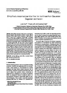
Figure 1: The relationship between several basic filter methods.

UPF estimate True x

Figure 2: The estimation result of PF, UPF, and AUPF.

2𝑁𝜀 >

2 𝜒𝑘−1,1−𝛿

󳨐⇒ 2

Var𝑝(𝑥) 𝑁𝐼𝑆 2 𝜎𝐼𝑆

󳨐⇒ 𝑁𝐼𝑆 >

Table 1: RMSE of AUPF, PF, and UPF.

>

2 𝜒𝑘−1,1−𝛿

Algorithm RMSE

2 𝜎𝐼𝑆 𝜒2 . 2𝜀Var𝑝(𝑥) 𝑘−1,1−𝛿

(16) min can be So the minimum number of particles 𝑁𝐼𝑆 obtained according to

min 𝑁𝐼𝑆 =⌈

2 𝜎𝐼𝑆 𝜒2 ⌉. 2𝜀Var𝑝(𝑥) 𝑘−1,1−𝛿

(17)

4.3. An Adaptive Unscented Particle Filter Algorithm through Relative Entropy. Figure 1 illustrates the relationship between several basic methods. The adaptive unscented particle filter algorithm through relative entropy is shown in Algorithm 2.

5. Experimental Results In this section, the results of two experiments are presented. In the first experiment the performance of AUPF is compared with UPF and PF through a simulation to validate the effectiveness of AUPF. Then the utilization and performance of AUPF for a real robot self-localization are also illustrated in detail. 5.1. Simulation Results. To illustrate the effectiveness of the proposed AUPF, a scalar nonlinear system is considered which is shown in (18) and (19). The simulation is carried out

AUPF 0.30687

PF 0.73439

UPF 0.28767

in an HP computer with 4 G memory and Intel Core i2-2120 CPU 𝑥𝑡 = 2 + sin (0.02𝜋𝑡) + 0.3𝑥𝑡−1 + 𝑤𝑡−1 , 𝑧𝑡 = {

0.2𝑥𝑡2 + V𝑡−1 , 𝑡 ≤ 30, 0.5𝑥 + V𝑡−1 , 𝑡 > 30.

(18) (19)

Equation (18) is the state transition model. Equation (19) is the state observation model. 𝑤𝑡 is white Gaussian noise, and its covariance is 1.5; V𝑡 is white Gaussian noise, and its covariance is 1. We compare the AUPF with traditional PF and UPF. The number of particles in PF and UPF is set to be 100. The initial number of particles in AUPF is also set to be 100. In the experiment we use a value 0.99 for 𝛿 and a fixed bin size Δ 0.02. Random 50-step state estimation results are shown in Figure 2. The root mean square error (RMSE) is an important value that can be used to reflect the accuracy of state estimation. RMSE can be calculated by 𝑡𝑓

2

∑ (𝑥 − 𝑥) . RMSE = √ 𝑡=1 𝑡𝑓

(20)

We have run AUPF, UPF, and PF for 10000 steps; the RMSE of the three algorithms is shown in Table 1. Meanwhile the average number of particles of the three algorithms is shown in Table 2. From Figure 2 and Table 1 we can see that the estimation result of PF is not satisfying. Particle filter uses a set

6

Mathematical Problems in Engineering

𝑖 𝑖 Inputs: 𝑆𝑡−1 = {(𝑥𝑡−1 , 𝑤𝑡−1 ) 𝑖 = 1, . . . , 𝑛}; the control measurement 𝑢𝑡−1 ; the observation 𝑧𝑡 ; the bound 𝜀 and the probability 𝜎; the bin size ℎ; 𝑆𝑡 = 𝜙; 𝑛 = 0; 𝑘 = 0; 𝛼 = 0. Generate the particles: 𝑖=1 do Sample a particle index 𝑗(𝑛) from the discrete distribution according to the weights in 𝑆𝑡−1 . 𝑗(𝑛) Obtain the particles 𝑥𝑡𝑛 from the particles 𝑥𝑡−1 according to (1). Compute the importance weight: 𝑤𝑡𝑛 = 𝑝(𝑧𝑡 | 𝑥𝑡𝑛 ) 𝛼 = 𝛼 + 𝑤𝑡𝑛 Insert particles into the particle set: 𝑆𝑡 = 𝑆𝑡 ∪ {(𝑥𝑡𝑛 , 𝑤𝑡𝑛 )} if (𝑥𝑡𝑛 falls into empty bin) 𝑘=𝑘+1 end if 𝑛=𝑛+1 2 ) while (𝑛 < (𝜎IS2 /2𝜀Var𝑝(𝑥) ) 𝜒𝑘−1,1−𝛿 Normalize the importance weight: for 𝑖 = 1, . . . , 𝑛 𝑤𝑡𝑖 = 𝑤𝑡𝑖 /𝛼 return 𝑆𝑡

Algorithm 2

Table 2: Average number of particles of AUPF, PF, and UPF. Algorithm Average number of particles

AUPF 69

PF 100

UPF 100

of particles to represent the posterior distribution, so the accuracy of PF is decided by the number of particles. In this experiment the number of particles is 100, and these particles cannot approximate the true posterior density well especially when the nonlinearity of the system is strong. The performance of UPF is the most excellent, because in this algorithm the latest observation is incorporated into the proposal distribution, so 100 particles are enough to approximate the true posterior density. In Table 2 the average number of particles of PF and UPF is 100; it is a fixed number of these algorithms, while in AUPF this number is adaptively adjusted according to (17). According to the adaptive adjustment of the number of particles the runtime of AUPF is reduced which is proportional to this number. 5.2. AUPF for Real Mobile Robot Self-Localization. We hereafter experimentally validate the effectiveness of AUPF for mobile robot self-localization. The robot “E-Robot” which is developed by Chinese Academy of Sciences is utilized for mobile robot self-localization. E-Robot is shown in Figure 3. During the mobile robot self-localization, the odometer information and the visual information are used. The picture is obtained by the ultrahigh definition color gun camera AMPSON DSC-B468C, and it is processed by FPGA Cyclone II EP2C20. The image pixel of the picture obtained by the camera is 256 ∗ 256. In one second about 30 pictures can be processed.

Figure 3: The E-Robot used in the experiments.

5.2.1. Mobile Robot Motion Model. The odometer can obtain the offset of robot pose (Δ𝑥𝑟, Δ𝑦𝑟, and Δ𝜃𝑟) from time 𝑡 − 1 to time t, so the motion model of mobile robot can be represented by 𝑥𝑟𝑡 = 𝑥𝑟𝑡−1 + Δ𝑥𝑟 + Δ𝑥𝑟 ∗ 𝛿𝑥𝑟 , 𝑦𝑟𝑡 = 𝑦𝑟𝑡−1 + Δ𝑦𝑟 + Δ𝑦𝑟 ∗ 𝛿𝑦𝑟 ,

(21)

𝜃𝑟𝑡 = 𝜃𝑟𝑡−1 + Δ𝜃𝑟 + Δ𝜃𝑟 ∗ 𝛿𝜃𝑟 , where (𝑥𝑟𝑡 , 𝑦𝑟𝑡 ) is the position at time step t; 𝜃𝑟𝑡 is the orientation at time step t; 𝛿𝑥𝑟 , 𝛿𝑦𝑟 , and 𝛿𝜃𝑟 are non-Gaussian noise. 5.2.2. Mobile Robot Observation Model. In our experiment, the mobile robot can move under an environment with many features, such as the white line and the two-dimension codes. All the features can be extracted from robot vision information.

Mathematical Problems in Engineering

7

(a) Example 1

(b) Example 2

(c) Example 3

(d) Example 4

Figure 4: Some examples of 2D code developed by Chinese Academy of Science.

In this paper, the special two-dimension (2D) codes have been used as the features or landmarks. As shown in Figure 4, the outer contour of each 2D code is regular pentagon. A different 2D code has different dots inside the regular pentagon. The 2D code is developed by Institute of Automation, Chinese Academy of Sciences. It is easy to be processed and can bring plenty of information. In [28], the image processing for 2D code is explained in detail. In our experiments, each 2D code is different from the others. Each 2D code is located at a fixed position, and it brings the location information. So once the mobile robot detects one 2D code, it can obtain one numerical value of selflocalization with the help of image processing. Assume that the robot can detect 𝑛 two-dimension codes 𝑑1 , . . . , 𝑑𝑛 , then 𝑛 self-localization value 𝑙V1 , . . . , 𝑙V𝑛 can be obtained accordingly. In our experiment, the mobile robot self-localization result is represented by a set of particles, 𝑠𝑗𝑡 = ⟨𝑙𝑝𝑗𝑡 , 𝑝𝑗𝑡 ⟩, where 𝑙𝑝𝑗𝑡 means the self-localization value maintained by the jth particle at time step t, and 𝑝𝑗𝑡 is the importance weight of the jth particle at time step t. Utilizing the mobile robot motion model and 𝑙𝑝𝑗𝑡−1 , the jth particle can obtain an original selflocalization numerical value 𝑙𝑝𝑜𝑗𝑡 . If the robot is localized at 𝑙𝑝𝑜𝑗𝑡 , the distance between 𝑙𝑝𝑜𝑗𝑡 and 𝑙V𝑖 can be used to calculate the probability 𝑃(𝑑𝑖 | 𝑙𝑝𝑜𝑗𝑡−1 ) with which the robot localized at 𝑙𝑝𝑜𝑗𝑡 can observe the feature 𝑑𝑖 . The probability will become bigger along with the decrease of the distance 𝑡

𝑃 (𝑑𝑖 | 𝑙𝑝𝑜𝑗𝑡−1 ) = e−|𝑙V𝑖 −𝑙𝑝𝑜𝑗 | .

(22)

The extraction of the features just depends on the robot’s position and orientation, so the features are mutually independent. The observation model 𝑃(𝑑 | 𝑙𝑝𝑜𝑗𝑡−1 ) is formulated in 𝑃 (𝑑 | 𝑙𝑝𝑜𝑗𝑡−1 ) = 𝑃 (𝑑1 | 𝑙𝑝𝑜𝑗𝑡−1 ) ∗ ⋅ ⋅ ⋅ ∗ 𝑃 (𝑑𝑛 | 𝑙𝑝𝑜𝑗𝑡−1 ) 𝑡

𝑡

= e−|𝑙V1 −𝑙𝑝𝑜𝑗 | ∗ ⋅ ⋅ ⋅ ∗ e−|𝑙V𝑛 −𝑙𝑝𝑜𝑗 | .

realization for mobile robot self-localization is reported as follows. (1) Obtain the initial position of the mobile robot 𝑙0 according to the robot vision. (2) Around 𝑙0 a field of 2 ∗ 2 meters is chosen, and 400 particles are uniformly distributed in this field; the importance weight of each particle is 1/400. (3) Obtain new particles according to UKF algorithm and the mobile robot motion model which utilizes the odometer information. (4) Obtain the vision information, extract the features, and update the importance weight of each particle according to (17). (5) Output the estimation of mobile robot position according to (18), then calculate the orientation of the robot according to (24), and then return to step 3 at the next time step. (6) Calculate the number of particles 𝑁𝑝𝑡 . (7) Resample 𝑁𝑝𝑡 particles according to their importance weight. (8) Set all the importance weight of particles to be 1/𝑁𝑝𝑡 . The robot position (𝑥𝑟𝑡 , 𝑦𝑟𝑡 ) is obtained by AUPF; then the orientation 𝜃𝑟𝑡 can be calculated according to 𝑥𝑙𝑡𝑟 = (𝑥𝑙 − 𝑥𝑟𝑡 ) cos 𝜃𝑟𝑡 − (𝑦𝑙 − 𝑦𝑟𝑡 ) sin 𝜃𝑟𝑡 , 𝑦𝑙𝑡𝑟 = (𝑥𝑙 − 𝑥𝑟𝑡 ) sin 𝜃𝑟𝑡 + (𝑦𝑙 − 𝑦𝑟𝑡 ) cos 𝜃𝑟𝑡 ,

(24)

where (𝑥𝑙, 𝑦𝑙) is the position of one 2D code in the world coordinate, and this position is already known. All the positions used above are in the world coordinate. (𝑥𝑙𝑡𝑟 , 𝑦𝑙𝑡𝑟 ) is the position of the 2D code in the robot coordinate, and this position can be easily obtained by the image processing.

(23)

Actually, the mobile robot can detect at least one feature in our experiment, and no more than two features will be chosen which are the nearest to the robot. 5.2.3. The Realization of AUPF for Mobile Robot Self-Localization. In the experiment, the initial number of particles of AUPF is set to be 400. The number of particles during filtering at time instant t is represented by 𝑁𝑝𝑡 . The process of the

5.2.4. Experiment Results and Analysis. In order to illustrate the effectiveness of AUPF, we designed a mobile robot selflocalization experiment. In the experiment, the E-Robot randomly moved on the ground, and a trajectory was generated. Then the trajectory was recorded. The trajectory is depicted in Figure 5 by a black line. From Figure 5 we can see that the 2D codes are located on the ground as landmarks. When the robot moved, AUPF was run to calculate the robot position at each time step. The effect of AUPF can be measured by the difference between the calculated position and the trajectory.

8

Mathematical Problems in Engineering 3 2.5

y (m)

2 1.5 1

Figure 5: The real trajectory of the E-Robot in the experiment.

0.5 0

Table 3: Experiment results of AUPF, PF, and UPF. Algorithm MRPE Average run time (ms) Average number of particles

AUPF 9.62 3.396 298

PF 18.91 2.262 400

Then we adopt AUPF, UPF, and PF to obtain the estimation of self-localization value. The estimation results of the three algorithms are shown in Figure 6. The mobile robot self-localization result can be measured by the mean relative position error (MRPE) which is defined in 2

𝑡𝑓

MRPE =

𝑡𝑓

2

,

0.5

1

1.5

2

2.5

3

3.5

4

4.5

5

x (m)

UPF 7.86 4.635 400

𝑡 𝑡 − 𝑥̂𝑡 ) + (𝑦true − 𝑦̂𝑡 ) ∑𝑡=1 √(𝑥true

0

(25)

𝑡 𝑡 and 𝑦true are the true robot positions in Cartesian where 𝑥true coordinates at time step t, tf is the total time instant of the three algorithms, and 𝑥̂𝑡 and 𝑦̂𝑡 are the estimation results. From Figure 6 and Table 3 we can see that the MRPE of AUPF is better than PF, and the MRPE of UPF is the best. That is, because in UPF each particle moves according to a new proposal distribution which utilizes the new observation, while in PF the particles cannot move appropriately without the direction of new observation. We also find that AUPF can acquire relatively ideal accuracy. The number of particles in AUPF is reduced, and the reduction is according to the estimation quality, so the reduction will not cause severe loss of accuracy.

6. Conclusions In UPF the number of particles is fixed, and the computation cost of UPF is relatively large which influences its realtime capability. In order to accommodate the mobile robot self-localization under dynamic environment, an adaptive unscented particle filter algorithm through relative entropy has been proposed in this paper. This algorithm utilizes the concept of relative entropy to measure the distance between the empirical distribution and the true posterior; then the difference between the proposal distribution and the true distribution is offset to obtain the least number of particles of UPF for the next step. This algorithm can effectively reduce the computation cost and enhance the real-time capability for UPF. In the future, we will research on how to further reduce

True value of self-localization The result of AUPF

The result of PF The result of UPF

Figure 6: The estimation results of PF, UPF, and AUPF.

the computation of UPF at the least cost of the accuracy. Moreover, the influence of the accuracy will be investigated and analyzed.

Acknowledgments The authors would like to thank Professor Jing Wang for his work on the paper revision. This paper is supported by the National Natural Science Foundation of China (nos. 61071096, 61073103, and 61202342), Research Fund for the Doctoral Program of Higher Education of China (nos. 20110162110042 and 20100162110012), and the Science and Technology Planning Project of Hunan Province, China (no. 2011GK3214).

References [1] A. Finn, A. Jacoff, M. Del Rose et al., “Evaluating autonomous ground-robots,” Journal of Field Robotics, vol. 29, no. 5, pp. 689– 706, 2012. [2] S. Thrun, S. Thayer, W. Whittaker et al., “Autonomous exploration and mapping of abandoned mines: software architecture of an autonomous robotic system,” IEEE Robotics and Automation Magazine, vol. 11, no. 4, pp. 79–91, 2004. [3] R. Siegwart and I. R. Nourbakhsh, Introduction to Autonomous Mobile Robots, MIT Press, London, UK, 2004. [4] S. S. Ge and F. L. Lewis, Autonomous Mobile Robots: Sensing, Control, Decision-Making, and Applications, CRC Press, Boca Raton, Fla, USA, 2006. [5] S. Thrun, W. Burgard, and D. Fox, Probabilistic Robotics, MIT Press, Cambridge, Mass, USA, 2006. [6] D. C. K. Yuen and B. A. MacDonald, “Vision-based localization algorithm based on landmark matching, triangulation, reconstruction, and comparison,” IEEE Transactions on Robotics, vol. 21, no. 2, pp. 217–226, 2005. [7] A. N. Raghavan, H. Ananthapadmanaban, M. S. Sivamurugan, and B. Ravindran, “Accurate mobile robot localization in indoor environments using bluetooth,” in Proceedings of the IEEE International Conference on Robotics and Automation (ICRA ’10), pp. 4391–4396, May 2010.

Mathematical Problems in Engineering [8] J. Wang, Q. Gao, Y. Yu, H. Wang, and M. Jin, “Toward robust indoor localization based on Bayesian filter using chirp-spreadspectrum ranging,” IEEE Transactions on Industrial Electronics, vol. 59, no. 3, pp. 1622–1629, 2012. [9] D. Fox, J. Hightower, L. Liao, D. Schulz, and G. Bordello, “Bayesian filtering for location estimation,” IEEE Pervasive Computing, vol. 2, no. 3, pp. 24–33, 2003. [10] Z. Chen, “Bayesian filtering: from Kalman filters to particle filters, and beyond,” Statistics, vol. 182, no. 1, pp. 1–69, 2003. [11] H. Zhang, G. Liu, T. W. S. Chow, and W. Liu, “Textual and visual content-based anti-phishing: a Bayesian approach,” IEEE Transactions on Neural Networks, vol. 22, no. 10, pp. 1532–1546, 2011. [12] D. M. Gavrila, “A Bayesian, exemplar-based approach to hierarchical shape matching,” IEEE Transactions on Pattern Analysis and Machine Intelligence, vol. 29, no. 8, pp. 1408–1421, 2007. [13] G. Bishop and G. Welch, “An introduction to the Kalman filter,” in Proceedings of the SIGGRAPH, Course 8, 2001. [14] E. Ivanjko, A. Kitanov, and I. Petrovic, “Model based Kalman filter mobile robot self-localization,” in Robot Localization and Map Building,, InTech, Rijeka, Croatia, 2010. ˇ [15] L. Tesli´c, I. Skrjanc, and G. Klanˇcar, “EKF-based localization of a wheeled mobile robot in structured environments,” Journal of Intelligent and Robotic Systems, vol. 62, no. 2, pp. 187–203, 2011. [16] B. F. La Scala and R. R. Bitmead, “Design of an extended Kalman filter frequency tracker,” IEEE Transactions on Signal Processing, vol. 44, no. 3, pp. 739–742, 1996. [17] R. Kandepu, B. Foss, and L. Imsland, “Applying the unscented Kalman filter for nonlinear state estimation,” Journal of Process Control, vol. 18, no. 7-8, pp. 753–768, 2008. [18] A. Giannitrapani, N. Ceccarelli, F. Scortecci, and A. Garulli, “Comparison of EKF and UKF for spacecraft localization via angle measurements,” IEEE Transactions on Aerospace and Electronic Systems, vol. 47, no. 1, pp. 75–84, 2011. [19] X. Shao, B. Huang, and J. M. Lee, “Constrained Bayesian state estimation—a comparative study and a new particle filter based approach,” Journal of Process Control, vol. 20, no. 2, pp. 143–157, 2010. [20] R. Karlsson, G. Hendeby, and F. Gustafsson, “Particle filtering: the need for speed,” Eurasip Journal on Advances in Signal Processing, vol. 2010, Article ID 181403, 2010. [21] X. Zhang, J. Peng, W. Yu, and K. C. Lin, “Confidence-levelbased new adaptive particle filter for nonlinear object tracking,” International Journal of Advanced Robotic Systems, vol. 9, no. 199, pp. 1–19, 2012. [22] J. Liu, C. Han, F. Han, and Y. Hu, “Multiple maneuvering target tracking by improved particle filter based on multiscan JPDA,” Mathematical Problems in Engineering, vol. 2012, Article ID 372161, 25 pages, 2012. [23] R. Merwe, A. Doucet, J. Freitas, and E. Wan, “The unscented particle filter,” Advances in Neural Information Processing Systems, vol. 13, no. 8, pp. 351–3357, 2000. [24] K. Yuan, Y. Li, and L. X. Fang, “Multiple mobile robot systems: a survey of recent work,” Acta Automatica Sinica, vol. 33, no. 8, pp. 785–794, 2007. [25] T. M. Cover and J. A. Thomas, Elements of Information Theory, John Wiley & Sons, New York, NY, USA, 1991. [26] J. Fan, C. Zhang, and J. Zhang, “Generalized likelihood ratio statistics and wilks phenomenon,” Annals of Statistics, vol. 29, no. 1, pp. 153–193, 2001.

9 [27] J. Geweke, “Evaluating the accuracy of sampling-based approaches to the calculation of posterior moments,” in Proceedings of the 4th Valencia International Meeting, pp. 88–169, 1992. [28] R. Zheng, K. Yuan, and Y. Li, “2D code for mobile robot localization and navigation in indoor environments,” Chinese High Technology Letters, vol. 18, no. 4, pp. 369–374, 2008.

Advances in

Operations Research Hindawi Publishing Corporation http://www.hindawi.com

Volume 2014

Advances in

Decision Sciences Hindawi Publishing Corporation http://www.hindawi.com

Volume 2014

Journal of

Applied Mathematics

Algebra

Hindawi Publishing Corporation http://www.hindawi.com

Hindawi Publishing Corporation http://www.hindawi.com

Volume 2014

Journal of

Probability and Statistics Volume 2014

The Scientific World Journal Hindawi Publishing Corporation http://www.hindawi.com

Hindawi Publishing Corporation http://www.hindawi.com

Volume 2014

International Journal of

Differential Equations Hindawi Publishing Corporation http://www.hindawi.com

Volume 2014

Volume 2014

Submit your manuscripts at http://www.hindawi.com International Journal of

Advances in

Combinatorics Hindawi Publishing Corporation http://www.hindawi.com

Mathematical Physics Hindawi Publishing Corporation http://www.hindawi.com

Volume 2014

Journal of

Complex Analysis Hindawi Publishing Corporation http://www.hindawi.com

Volume 2014

International Journal of Mathematics and Mathematical Sciences

Mathematical Problems in Engineering

Journal of

Mathematics Hindawi Publishing Corporation http://www.hindawi.com

Volume 2014

Hindawi Publishing Corporation http://www.hindawi.com

Volume 2014

Volume 2014

Hindawi Publishing Corporation http://www.hindawi.com

Volume 2014

Discrete Mathematics

Journal of

Volume 2014

Hindawi Publishing Corporation http://www.hindawi.com

Discrete Dynamics in Nature and Society

Journal of

Function Spaces Hindawi Publishing Corporation http://www.hindawi.com

Abstract and Applied Analysis

Volume 2014

Hindawi Publishing Corporation http://www.hindawi.com

Volume 2014

Hindawi Publishing Corporation http://www.hindawi.com

Volume 2014

International Journal of

Journal of

Stochastic Analysis

Optimization

Hindawi Publishing Corporation http://www.hindawi.com

Hindawi Publishing Corporation http://www.hindawi.com

Volume 2014

Volume 2014