ential pulse code modulation (DPCM) and vector quantization (VQ) in a ..... Other lossless compression techniques include run-length coding, contour coding,.
An Algorithm for Image Compression Using Differential Vector Quantization A Thesis Presented in Partial Ful llment of the Requirements for the Degree Master of Science in the Graduate School of The Ohio State University by James E. Fowler, Jr., B. S. ***** The Ohio State University 1995 Master's Examination Committee: Stanley C. Ahalt Ashok K. Krishnamurthy
Approved by Adviser Department of Electrical Engineering
To my parents
ii
THESIS ABSTRACT THE OHIO STATE UNIVERSITY GRADUATE SCHOOL NAME: Fowler, James E., Jr. DEPARTMENT: Electrical Engineering
QUARTER/YEAR: SP 92 DEGREE: M. S.
ADVISER'S NAME: Ahalt, Stanley C. TITLE OF THESIS: An Algorithm for Image Compression Using Di�erential Vector Quantization
There has been recent interest in image compression for scienti c applications. An algorithm for compression of single, monochrome images which preserves salient image features such as edges is discussed. The algorithm described combines di�erential pulse code modulation (DPCM) and vector quantization (VQ) in a method called di�erential vector quantization (DVQ). An Arti cial Neural Network (ANN) is used to train codebooks for the vector quantizer. Such ANN training is shown to produce codebooks with entropy su�cient that subsequent Hu�man coding cannot provide signi cant additional compression. Consequently, the DVQ algorithm provides compression rates similar to those achieved by scalar DPCM methods while remaining robust to transmission channel errors.
Adviser's Signature Department of Electrical Engineering
Acknowledgments I would like to thank Dr. Stan Ahalt and Dr. Ashok Krishnamurthy for the invaluable guidance and motivation provided. Also, I would like to thank Matt Carbonara for help with the DVQ codebook training process. Finally, I thank the Ohio State University and the Ohio Space Grant Consortium for providing me graduate fellowships in support of this research.
iii
Vita January 19, 1967 : : : : : : : : : : : : : : : : : : : : : Born|Huntsville, Alabama, U.S.A. 1985 { 1990 : : : : : : : : : : : : : : : : : : : : : : : : : : Ohio Academic Scholar The Ohio State University Columbus, Ohio, U.S.A. March 1990 : : : : : : : : : : : : : : : : : : : : : : : : : : : B. S. Computer and Information Science Engineering, Summa Cum Laude The Ohio State University Columbus, Ohio, U.S.A. 1991 { Present : : : : : : : : : : : : : : : : : : : : : : : : NASA Space Grant/OAI Fellowship Ohio Space Grant Consortium 1990 { Present : : : : : : : : : : : : : : : : : : : : : : : : University Fellow The Ohio State University Columbus, Ohio, U.S.A.
Publications \Compiled Instruction Set Simulation," in Software{Practice and Experience, Vol. 21, pp. 877{889, August 1991 (with Christopher Mills and Stanley C. Ahalt).
Fields of Study Major Field: Electrical Engineering iv
Studies in Communications:
Professors R. L. Moses, L. C. Potter A. K. Krishnamurthy, K. L. Boyer
Studies in Computer Engineering:
Professors S. C. Ahalt, F. O zguner
v
Table of Contents DEDICATION : : : : : : : : : : : : : : : : : : : : : : : : : : : : : : : : : : : ii ACKNOWLEDGMENTS : : : : : : : : : : : : : : : : : : : : : : : : : : : : : iii VITA : : : : : : : : : : : : : : : : : : : : : : : : : : : : : : : : : : : : : : : : iv LIST OF FIGURES : : : : : : : : : : : : : : : : : : : : : : : : : : : : : : : : viii LIST OF TABLES : : : : : : : : : : : : : : : : : : : : : : : : : : : : : : : : : x CHAPTER I
PAGE
INTRODUCTION : : : : : : : : : : : : : : : : : : : : : : : : : : : : : : 1.1 Types of Image Compression Techniques 1.1.1 Lossless Image Compression : : : 1.1.2 Predictive Techniques : : : : : : 1.1.3 Transform Coding : : : : : : : : 1.2 Algorithm Objectives : : : : : : : : : : 1.3 A Scalar DPCM Algorithm : : : : : : :
II
: : : : : :
: : : : : :
: : : : : :
: : : : : :
: : : : : :
: : : : : :
: : : : : :
: : : : : :
: : : : : :
: : : : : :
: : : : : :
: : : : : :
: : : : : :
: : : : : :
: : : : : :
1 3 3 5 8 10 12
BACKGROUND THEORY : : : : : : : : : : : : : : : : : : : : : : : : : 16 2.1 Vector Quantization : : : : : : : : : : : : : : : : : : : : : : : : : : 16 2.2 Arti cial Neural Networks and Vector Quantization : : : : : : : : : 20 2.3 Di�erential Vector Quantization : : : : : : : : : : : : : : : : : : : : 21
III DVQ Algorithm Details : : : : : : : : : : : : : : : : : : : : : : : : : : : 24 3.1 Prediction : : : : : : : : : : : : : : : : : : : : : : : : : : : : : : : : 24 3.2 Codebook Design : : : : : : : : : : : : : : : : : : : : : : : : : : : : 28 vi
IV Results : : : : : : : : : : : : : : : : : : : : : : : : : : : : : : : : : : : : : 29 4.1 Prediction : : : : : : : : : : : : : : : : : : : : : : : : : : : : : : : : 29 4.2 Comparison to scalar DPCM : : : : : : : : : : : : : : : : : : : : : 32 4.3 Codebook Entropies : : : : : : : : : : : : : : : : : : : : : : : : : : 38 V
CONCLUSIONS AND FUTURE RESEARCH : : : : : : : : : : : : : : : 40
REFERENCES : : : : : : : : : : : : : : : : : : : : : : : : : : : : : : : : : : : 42
vii
List of Figures
FIGURE
PAGE
1
Image compression system block diagram : : : : : : : : : : : : : : : :
2
2
DPCM block diagram : : : : : : : : : : : : : : : : : : : : : : : : : :
6
3
Scalar DPCM algorithm block diagram : : : : : : : : : : : : : : : : : 13
4
Scalar DPCM predictor : : : : : : : : : : : : : : : : : : : : : : : : : : 14
5
Vector quantization conceptual diagram : : : : : : : : : : : : : : : : 17
6
Di�erential vector quantizer algorithm block diagram : : : : : : : : : 22
7
Pixels used in the prediction schemes : : : : : : : : : : : : : : : : : : 25
8
FSCL training procedure : : : : : : : : : : : : : : : : : : : : : : : : : 28
9
Lenna, original image : : : : : : : : : : : : : : : : : : : : : : : : : : : 34
10 Reconstructed image using the scalar DPCM algorithm : : : : : : : : 34 11 Reconstructed image using the DVQ algorithm (256 codewords) : : : 35 12 Di�erence between the reconstructed scalar DPCM image and the original image (enhanced) : : : : : : : : : : : : : : : : : : : : : : : : 35 13 Di�erence between the reconstructed DVQ image and the original image (enhanced) : : : : : : : : : : : : : : : : : : : : : : : : : : : : : 36 14 Reconstructed image with an error-prone channel, scalar DPCM algorithm, ber = 1000 : : : : : : : : : : : : : : : : : : : : : : : : : : : 36 viii
15 Reconstructed image with an error-prone channel, DVQ algorithm (256 codewords), ber = 1000 : : : : : : : : : : : : : : : : : : : : : : : 37
ix
List of Tables
TABLE
PAGE
1
Prediction equations for encoding and decoding : : : : : : : : : : : : 26
2
Mean squared error (MSE) of the prediction schemes : : : : : : : : : 30
3
MSE of the prediction schemes with individually tailored codebooks : 31
4
MSE of scalar DPCM and DVQ algorithms : : : : : : : : : : : : : : : 32
5
Codebook entropies for DVQ : : : : : : : : : : : : : : : : : : : : : : : 39
x
CHAPTER I INTRODUCTION Digital images are becoming quite prevalent in our society and can take the form of both still pictures (single frames) or motion video (sequences of frames). Still digital images arise in applications such as medicine (computer tomography, magnetic resonance imaging, and digital radiology), satellite data, weather prediction, facsimile transmission, electronic cameras, and multimedia software [1, 2]. Digital motion video has been used in broadcast television, teleconferencing, and video-phone technologies [1, 2]. Despite the di�ering contexts of use, these digital images have one thing in common { invariably, they are comprised of an enormous amount of data. Reduction of the size of this data for both the storing and transmission of digital images is becoming increasingly important as these images nd more applications. Image compression refers to the reduction of the size of data that images contain. Generally, image compression schemes exploit certain data redundancies to convert the image to a smaller form. A typical image compression system is shown in Figure 1. The data reduction, or compression, is performed by a device known as the encoder. The encoder reduces the data size of the original image, outputting a compressed image. The compressed image passes through a channel (usually 1
2 an actual transmission channel or a storage system) to the decoder. The decoder reconstructs, or decompresses, the image from the compressed data. The ratio of the size (amount of data or bandwidth) of the original image to the size of the compressed image is known as the compression ratio or compression rate. The higher the compression rate, the greater the reduction of data. Depending on the application, the channel may be a�ected by noise which results in distortion of the compressed image during transmission. If so, the channel is known as an error-prone channel; otherwise, it is errorless. Original Image
Encoder
Compressed Image
Channel
Reconstructed Image
Decoder
Figure 1: Image compression system block diagram This paper describes an image compression algorithm known as di�erential vector quantization (DVQ). The rst sections of the paper provide a general overview of di�erent types of image compression and some background theory used in the development of the algorithm. The details of the algorithm are presented next,
3 followed by the experimental results and conclusions.
1.1 Types of Image Compression Techniques There are many compression techniques, but they may be partitioned into the three general categories of lossless, predictive, and transform coding algorithms. A general description of these categories and their use in image compression applications follows.
1.1.1 Lossless Image Compression In lossless image compression, the reconstructed image output by the decoder is exactly the same as the original image input to the encoder, provided the channel is errorless. Usually lossless algorithms code pixel intensities, although, when used in conjunction with other techniques, they can code other quantities. One form of lossless compression is Hu�man coding. In this technique, it is assumed that each pixel intensity has associated with it a certain probability of occurring and this probability is spatially invariant. Hu�man coding assigns a binary code to each intensity value, with shorter codes going to intensities with higher probability [3]. If the probabilities can be estimated a priori, then the table of Hu�man codes can be xed in both the encoder and the decoder. Otherwise, the coding table must be sent to the decoder along with the compressed image data. The compression rate of Hu�man coding is limited by the entropy of the pixels.
4 Pixel entropy is de ned as
N X H = ? pi log2 pi
(1.1) i=1 where pi is the probability of occurrence of the ith intensity level, and N is the number of possible pixel intensity levels. By Shannon's noiseless coding theorem, it is possible to code, without distortion, these pixel intensities with an average of
H + � bits/pixel, where � > 0 is an arbitrarily small quantity [1]. Entropy coding methods, of which Hu�man coding is the most e�cient, attempt to reduce the bit rate to as close to H as possible. Hu�man coding is lossless only when the channel is errorless. Since Hu�man coding employs a variable-length code scheme, it is possible for an error-prone channel to have serious detrimental e�ects. The only indication of code length is the code itself. Consequently, a channel error may cause the decoding to diverge signi cantly from the encoding as the decoder loses track of the code lengths or perceives an illegal code. This e�ect may be lessened by resynchronizing the decoder to the encoder periodically (such as at the end of each horizontal image line) [4]. Also, additional codes may be transmitted to allow for error detection at the expense of decreased compression rate [1]. Other lossless compression techniques include run-length coding, contour coding, arithmetic coding, and conditional replenishment [3]. Like Hu�man coding, they have limited compression ratios and so are used only in very sensitive applications (such as medical imagery) where data loss is unacceptable, or in conjunction with other techniques [2]. Because of their sensitivity to channel errors, lossless techniques
5 are e�ective only when channel errors are infrequent or the channel is errorless.
1.1.2 Predictive Techniques Adjacent pixels usually possess a high degree of spatial coherence; that is, the intensity values of adjacent pixels are highly correlated. Predictive techniques exploit this spatial coherence and encode only the new information between successive pixels [1]. Predictive algorithms feature a predictor which calculates a value from previously encoded pixels. This prediction is subtracted from the actual image value and the di�erence is encoded. The di�erence values typically have smaller dynamic range than the original image quantities, so they may be encoded using fewer bits per pixel [5]. One frequently used method of predictive image compression is di�erential pulse code modulation (DPCM). A DPCM encoder/decoder system is shown in Figure 2. In the encoder, the predictor calculates a predicted value, x~. The predicted value is subtracted from the input value to form the di�erence, d. The di�erence is quantized and passed through the channel. The quantized di�erence, d^, is added to the predicted value, x~, to form the reconstructed value, x^. Reconstructed values are used by the predictor in the calculation of the next predicted value. The decoder receives the quantized di�erence from the channel and calculates a reconstructed value using the same prediction loop as the encoder. DPCM may be performed on single pixels or blocks of pixels, in which case it is known as vector DPCM [1]. If image statistics are known and relatively stationary, the predictor may be
6
Input
x
+
d
^ d
Quantizer
−
+
~ x
^x Predictor +
Channel ENCODER
^ x
+
Output +
Predictor
~ x
DECODER
Figure 2: DPCM block diagram
7 made optimal in the mean square sense. However, for hardware implementations, a simpler averaging predictor involving integers and shift operations is usually used [1]. Generally, only the nearest neighbor pixels are used as additional, more distant pixels do not provide better prediction [1]. The quantizer in predictive algorithms is responsible for three types of distortions: granular noise, slope overload, and edge-busyness [1, 3]. Granular noise is a distortion of areas of near-constant intensity and occurs when the quantizer does not have su�cient quantization levels of small di�erence values. Slope overload occurs when the quantizer does not have a large enough level for large di�erence values that occur at sharp image edges. Edge-busyness occurs at less sharp edges when di�erent pixel rows are quantized di�erently. Channel errors are not con ned to the portion of the image in which they occur. The predictive process in the decoder tends to \smear" the error to other parts of the image. If causal prediction is used in scan-line based DPCM, this smearing occurs to lower right from the point of error occurrence. Predictive techniques, like lossless methods, are computationally simple and easily realized in hardware. Prediction yields relatively good compression ratios and may be used with transform coding or lossless image compression techniques to achieve additional compression. Also, the predictor may be changed on-line to compensate for varying image statistics; this scheme is known as adaptive prediction [1]. Practical DPCM algorithms have been developed for both scalar [4] and vector [5] architectures. Also, prediction may be performed between successive frames in
8 video compression. Techniques such as motion compensation employ such temporal prediction in the form of displacement estimations of objects within the moving image [1].
1.1.3 Transform Coding Transform coding is a mathematic operation that converts a large set of highly correlated pixels into a smaller set of uncorrelated coe�cients [1, 3]. Usually, the image is broken into blocks of M � N pixels, and the transform applied to each block separately. The two-dimensional transform operation can be represented as
F (u; v) =
MX?1 NX ?1 x=0 y=0
f (x; y)�uv (x; y)
(1.2)
where f (x; y) is the image data and the �uv (x; y) are a set of orthogonal basis vectors [3]. Usually, M = N and the transform is applied to square blocks. The variables
u and v may be thought of as spatial frequency variables and consequently F (u; v) as frequency coe�cients, although this frequency domain representation is accurate only when the basis vectors �uv (x; y) are the complex exponentials of the Fourier transform [3]. The image data may be losslessly recovered via the inverse transform
f (x; y) =
MX?1 NX ?1 u=0 v=0
F (u; v)�?xy1 (u; v)
(1.3)
where the �?xy1(u; v) are the basis vectors of the image [3]. Data compression occurs only after the transform coe�cients are quantized [3]. Some of the coe�cients, especially those of high spatial frequency, often have very
9 small magnitudes, and, consequently, are quantized very coarsely or omitted completely. Compression results from encoding the block of coe�cients with fewer bits than the original image block at the loss of some image delity by the quantization. Before transmission through the channel, the coe�cients may be entropy encoded for additional compression [3]. Of the many transforms available, several are commonly considered in image compression applications. The Karhunen-Lo�eve transform (KLT) is optimal in the sense that it minimizes the mean square distortion of the reconstructed image for a given number of bits [1]. However, KLT is rarely used in practice because of its substantial computational time and that di�erent basis vectors must be calculated for each image and sent with the image data [3]. The two-dimensional Fourier transform is not used for compression because it involves complex arithmetic; however, it is useful if a frequency domain representation is needed for analysis [1]. The discrete cosine transform (DCT) is often used in practical applications as its basis vectors are two-dimensional cosine functions and it yields performance near that of the KLT. Also, the arithmetic is real and there are \fast" computational algorithms available [1]. The sine, Hadamard, Haar, and slant transforms are other transforms that are sometimes used in image compression [1]. Generally, transform coding is capable of greater compression than predictive techniques [1]. Because of the block nature of the transform, distortions due to quantization and channel errors tend to be distributed throughout the block. If the block size is relatively small, these distortions are con ned to a small portion of the
10 image and may not be noticeable. However, these transforms tend to make edges \blocky," and, since the quantization tends to weight low over high spatial frequencies, edges and areas of texture may be blurred [3]. Transform techniques require much more computation than either lossless techniques or predictive techniques; however, recently several discrete cosine transform integrated circuit chips have become available which will reduce the complexity of hardware transform coders [2].
1.2 Algorithm Objectives Because of the many varied techniques, design of an image compression system must follow a careful consideration of the context within which the system will operate, the type of data it will process, and how it will be implemented. Some alternatives are: compression for storage versus bandwidth reduction; single, still images versus moving images (video); hardware implementation versus software; high rate of compression versus image quality; real-time versus batch processing; and a channel which is errorless versus an error-prone channel. The choices made will a�ect the types of compression techniques used in the design. For purposes of this paper, we will assume the following context. It is desired that an image compression algorithm be designed for compression of color television signals to be used in not only current video systems, but also forthcoming high de nition television (HDTV) and high resolution, high frame rate video technology (HHVT). It is expected that the algorithm will be used for scienti c purposes, so it is required that it achieve reasonable compression rates without
11 distorting salient features of the images. The following is an example of such an application. Scienti c experiments performed in space may be video recorded in an HHVT format. These video recordings may be recorded directly to tape or optical disk, or they may be transmitted to Earth. Because of limited bandwidth and storage space available to the spacecraft, image compression is needed. Since precision measurements will be made from these recordings, it is desired that features, such as edges and color content, be as little altered as possible, and channel errors cannot be ignored. Several examples of scienti c experiments to be performed in space and recorded with HHVT equipment are given in [3]. The goals for the image compression algorithm of the example above are as follows. Reconstructed images should be very high quality, especially, edges should be preserved not only in sharpness but also in location. The algorithm should be insensitive to channel errors. Although it may be assumed that such errors occur rather infrequently in real applications, the algorithm will be tested under conditions of a very noisy channel to assure robustness. Eventually, the algorithm will be built in hardware, so the algorithm should be computationally simple in order to permit hardware construction. Finally, the algorithm should process video images in real time so that substantial bu�ering (at additional implementation cost) is unnecessary. The image compression algorithm presented in this paper uses a combination of vector quantization (VQ) and di�erential pulse code modulation (DPCM), and is known as di�erential vector quantization (DVQ). It will be shown that this DVQ algorithm yields high quality images and is insensitive to channel errors. To simplify
12 the testing of the algorithm, still monochrome images were used during development. It is expected that temporal considerations for real-time video will be a straightforward addition to the basic algorithm.
1.3 A Scalar DPCM Algorithm The DVQ algorithm detailed in this paper was originally an adaptation of the popular di�erential pulse code modulation (DPCM) compression method. Scalar DPCM algorithms have been developed for practical video applications as they are wellsuited for real-time hardware implementation [1]. A scalar DPCM algorithm, designed for real-time video compression and implemented in hardware by NASA at Lewis Research Center, was chosen as a basis for comparison. This scalar DPCM image compression algorithm is described in depth in [4]. A brief description is given below. The scalar DPCM architecture processes NTSC composite color television signals in real time, averaging a compression of about 1.8 bits/pixel. The algorithm features nonuniform scalar quantization within a DPCM framework. Also, a nonadaptive predictor and a Hu�man coder are used to achieve greater compression than possible with DPCM alone. Figure 3 is a block diagram of the algorithm. The nonadaptive predictor generates a value, NAP , which is subtracted with the current predicted value, PV , from the current pixel, PIX , to yield the current di�erence, DIFF . The nonadaptive predictor generates this NAP value from the previous di�erence by indexing into a prestored array created from statistics of
13
Current Pixel
+
Σ
PIX
DIFF
Scalar Quantizer
−
QL
Huffman Coder
− Nonadapter Predictor
Inverse Scalar Quantizer
NAP
+ PIX
PV
Predictor
+
Σ
DIFF
+
ENCODER CHANNEL
Nonadapter Predictor NAP
+
Reconstructed Pixel
PIX
+
Σ
DIFF
Inverse Scalar Quantizer
QL
Inverse Huffman Coder
+
PV
Predictor
DECODER
Figure 3: Scalar DPCM algorithm block diagram
14 many images. The nonadaptive predictor improves the edge performance of DPCM because it results in quicker convergence at transition points in the image [4]. Figure 4 shows the pixels used by the codec predictor. The predictor averages the pixels above and to the left of the current pixel to generate the predicted value. B
C
A
PIX
Current Pixel
PV = A +2 C Figure 4: Scalar DPCM predictor The quantizer has 13 levels and is nonuniform, with more levels provided for small di�erence magnitudes. The Hu�man coder was designed so that the shortest transmitted codewords correspond to the quantization levels that have the highest probability of occurrence. Use of this Hu�man coding provides signi cant compression beyond what is obtainable with DPCM alone; however, since it features a variable-length code, it is susceptible to transmission errors. The experimental results obtained from the hardware implementation of this algorithm suggest that it performs quite well. The reconstructed images are nearly indistinguishable from the originals and the compression rate results in signi cant
15 bandwidth compression [4]. The DVQ algorithm described in this paper adds robustness to transmission errors to these advantages by replacing scalar quantization with more e�cient vector quantization.
CHAPTER II BACKGROUND THEORY 2.1 Vector Quantization The philosophy of vector quantization (VQ) stems from Shannon's rate-distortion theory which implies that, theoretically, better performance can always be obtained from coding vectors of information rather than scalars [6]. An extensive discussion of vector quantization techniques and applications is given in [6], and the basic theory is summarized in the context of image applications in [7, 8]. The basic conceptual diagram of a vector quantization system is presented in Figure 5. The VQ system consists of an encoder, a decoder, and a transmission channel. The encoder and the decoder each have access to a codebook, Y. The
codebook Y is a set of Y codewords (or codevectors), y, where each y is dimension
n2 and has a unique index, j , 0 � j � Y ? 1. The image is broken into blocks of pixels called tiles. Each image tile of n � n pixels can be considered a vector, u, of dimension n2. For each image tile, the
encoder selects the codeword y that yields the lowest distortion by some distortion
measure d(u; y). The index, j , of that codeword is sent through the transmission 16
17
Codebook Y
Input vector from image
u
Select codeword y from codebook Y that is closest to u Transmit index j of codeword y
j
ENCODING Transmission Channel Codebook Y
Output vector to ^ u reconstructed image
Retrieve codeword y from codebook Y that has index j Use codeword y in reconstructed image
j
DECODING
Figure 5: Vector quantization conceptual diagram
18 channel. If the channel is errorless, the decoder retrieves the codeword y associated
with index j and outputs y as the reconstructed image tile, u^.
Mathematically, VQ encoding is a mapping from a k-dimensional vector space to a nite set of symbols, J,
V Q : u = (u1 ; u2; : : : ; uk ) ! j
(2.1)
where k = n2 , j 2 J, and J has size J = Y . The rate, R, of the quantization is
R = log2 Y
(2.2)
where R is bits per input vector. The compression rate is R=n2 bits per pixel. Typically, Y is chosen to be a power of 2, so R is an integer. Consequently, VQ encoding generates codes of R bits in length with every R-bit code corresponding to some y 2 Y. Two common distortion measures are squared error k X dsq (u; y) = (ui ? yi )2 i=1 and absolute error
dabs (u; y) =
(2.3)
Xk ju ? y j
(2.4) i i i=1 The performance of a vector quantization system depends on the composition of the codebook [7]. Several criterions may be used to design an optimal codebook. It may be desired that the average distortion (typically mean squared error) due to VQ be minimized. Another criterion is to maximize the entropy of the codebook; that is, to ensure that each of the codewords is used equally frequently on the average [7]. Once the criterion is decided upon, the optimal codebook must be determined.
19 Typically, the probability distribution of the input images is not known, so the codebook is constructed by training [7]. During training, a set of representative input vectors (i.e. sample images) are used to determine the codebook. Typically, once the codebook is trained, it is xed in both the encoder and the decoder. However, in adaptive VQ, the codebook is modifed as image statistics change. New codewords are trained as the compression system is operating and these new codewords replace old ones in the codebook periodically. The encoder must inform the decoder of the changes made to the codebook in some way. In the past, vector quantization has had limited use in image compression applications because of the large computational expenses for the encoding and training processes [7]. In both processes, distortions are calculated for each codeword in the codebook and these distortions are compared to nd the closest codeword. Since these calculations must be performed for each input vector, the overall operation is quite computationally expensive. Another disadvantage to vector quantization is that, being block oriented, it tends to make the image edges \blocky" [5]. Vector quantization has several advantages in addition to its potential for signi cant bit rate reduction. It is possible to construct the codebook such that the entropy is maximized [7]. Because VQ produces xed length codes, such entropybased codebooks can be used to yield maximal-entropy encoding of the image without resorting to variable-length codes [7]. In addition, the codebook can be arranged so that codevectors that are close in Euclidean distance have code indices which are close in Hamming distance. The result is that when an error occurs, the decoder
20 selects a tile that is close (in the mean squared sense) to the one originally broadcast [7]. Thus, maximum compression (based on pixel entropy) is achieved and the coding is relatively error-insensitive.
2.2 Arti cial Neural Networks and Vector Quantization The computational complexity of traditional VQ codebook design methods has restricted their use in real-time applications [6, 9]. One such traditional approach is the Linde, Buzo, and Gray (LBG) algorithm [9] which is a locally-optimal algorithm that has been extensively used in designing vector quantizers for speech and image encoding. It has been proposed that Arti cial Neural Networks (ANNs) be used for design of VQ codebooks to circumvent the limitations of traditional algorithms [7]. ANNs consist of a large number of simple, interconnected computational units that can be operated in parallel. Also, ANN codebook design algorithms do not need access to the entire training data set at once during the training process. These features make ANN algorithms ideally suited for the design of adaptive vector quantizers [7]. One ANN, the Frequency-Sensitive Competitive Learning (FSCL) algorithm [10, 11], features a modi ed distortion measure that ensures all codewords in the codebook are updated equally frequently during iterations of the training process. Thus, the FSCL algorithm results in a codebook with maximum codeword entropy [7]. It has been shown that codebooks designed with FSCL yield mean squared errors and signal-to-noise ratios comparable to those of the locally-optimal LBG
21 algorithm in the vector quantizing of images [8]. Thus, it is expected that a FSCL ANN will yield codebooks with good mean-squared-error performance and with entropy su�cient that Hu�man coding of the VQ indices would not provide signi cant additional compression.
2.3 Di�erential Vector Quantization Di�erential Vector Quantization (DVQ) combines the methods of vector quantization (VQ) and di�erential pulse code modulation (DPCM). DVQ replaces the scalar quantizer in the DPCM framework with a vector quantizer, and consequently has many of the compression advantages of both VQ and DPCM. Figure 6 shows the general block diagram of the DVQ algorithm. The image to be compressed is processed in blocks, or tiles, of n � n pixels; these tiles may be considered vectors of dimension n2. In the encoding process, the predictor uses previously constructed tiles to predict the pixel values of the current tile. This predicted tile, PV , is subtracted pixel by pixel from the actual tile, PIX . The resulting di�erence tile, DIFF , is vector-quantized and the index, INDEX , is broadcast via the transmission channel to the decoder. The encoder inverse vector-quantizes ^ , to be used in later predictions. In INDEX , producing a reconstructed tile, PIX the decoding process, the index received from the transmission channel is inverse vector-quantized and the tile is reconstructed in the same manner as in the encoder. The inverse vector quantization step in the encoder is necessary so that the encoder tracks the operation of the decoder and predictions made in each process are iden-
22 tical. Note that the codebook for the vector quantizer contains di�erence tiles and must be trained appropriately on \di�erence images." Current Tile
+ Σ
PIX
DIFF
Vector Quantizer
INDEX
−
Inverse Vector Quantizer
PIX
PV
Predictor
+
Σ
DIFF
+
ENCODER CHANNEL
Reconstructed Tile
PIX
+
Σ
DIFF
Inverse Vector Quantizer
INDEX
+
PV
Predictor
DECODER
Figure 6: Di�erential vector quantizer algorithm block diagram DVQ has several advantages over both scalar DPCM and VQ. As discussed in Section 2.1, the quantization of vectors yields better compression performance than that of scalars. Additionally, since the vector quantization is performed on di�erence values rather than on the image itself, the resulting image is less \blocky"
23 [5]. Finally, the codebooks for DVQ tend to be more robust and more representative of many images than those codebooks designed for VQ because the di�erence tiles in a DVQ codebook are more generic than the image tiles in a VQ codebook [5].
CHAPTER III DVQ Algorithm Details The general architecture of the DVQ algorithm was depicted in Figure 6. There are two details remaining to complete the development of the algorithm. The design of the predictor and the method of constructing the codebook are discussed below.
3.1 Prediction All predictive techniques of image compression are an attempt to remove redundant information from the encoding process [1]. This redundant information is obtained from adjacent pixels, which are highly correlated, and subtracted from the pixel currently being encoded. Many predictor algorithms have been developed for scalar quantization, some of which are described in [1] and [3]. To be useful for di�erential vector quantization, these algorithms must be adapted to predict tiles rather than single pixels. The DVQ algorithm described here divides the image into tiles of 2 � 2 pixels, and processes these tiles in a raster-scan order. Several simple methods of causal prediction for tiles of this size were investigated. Figure 7 shows a typical tile and 24
25 the pixels from previously reconstructed tiles that were used in prediction. Previously reconstructed tiles
c
d
e
b
x 1
x
a
x 3
x
f
2 4
Current tile
Figure 7: Pixels used in the prediction schemes Table 1 presents the six prediction schemes that were studied and the names given to them for the purposes of the following discussion. Note that Table 1 shows the equations for both the encoding and decoding algorithms. Pred1 is an average twopixel predictor. Pred2, presented in [3], is similar to pred1, but uses reconstructed pixel values. Pred3, presented in [5], is also is similar to pred1, but uses previously predicted values. Pred4 is an average three-pixel predictor. Pred5 is an average four-pixel predictor. Pred6 is similar to pred4 in that it uses three pixels; however, it uses two divisions-by-two which are more conducive to hardware implementation than a division-by-three [1]. Except for pred2 and pred3, all the other predictors share an imperfection in that prediction is not done identically in the encoding and decoding processes. To illustrate, consider pred1, the average two-pixel predictor.
26
Table 1: Prediction equations for encoding and decoding Scheme pred1 pred2 pred3 pred4 pred5 pred6
Prediction
Encode x~1 = x~2 = x12+^e x~3 = a^+2x1 x1 Decode x~1 = x~2 = x^12+^e x~3 = a^+^ 2 ^ b +^ e a ^+d^ Encode x~1 = 2 x~2 = 2 x~3 = 2 ^ ^ b +d^ b +^ e Decode x~1 = 2 x~2 = 2 x~3 = a^+2 d^ ^ ^ x1 Encode x~1 = b+2 d x~2 = x~12+^e x~3 = a^+~ 2 ^ x ~1 +^ e a ^+~ b +d^ Decode x~1 = 2 x~2 = 2 x~3 = 2x1 ^ e+f x~2 = x1 +^ x~3 = a^+x31 +^e Encode x~1 = ^b+d3^+^e 3 ^ ^ ^ e+f Decode x~1 = b+d3+^e x~2 = x^1 +^ x~3 = a^+^x31 +^e 3 ^ ^ x1 +d^+^ e+f^ b +^ c +d^+^ e x~2 = x~3 = a^+b+4x1 +^e Encode x~1 = 4 4 x1 +^ e Decode x~1 = ^b+^c+4 d^+^e x~2 = x^1 +d^4+^e+f^ x~3 = a^+^b+^ 4 ^ ^ ^ e)=2 Encode x~1 = d+(b+^ x~2 = e^+(x12+f )=2 x~3 = x1 +(^a2+^e)=2 2 ^ ^ ^ e)=2 Decode x~1 = d+(b+^ x~2 = e^+(^x12+f )=2 x~3 = x^1 +(^a2+^e)=2 2 ^ b+d^ 2 ^ b+d^ 2 ^ b+d^
xi: actual pixel value (unencoded) x~i : predicted pixel value
x^i : reconstructed pixel value (decoded)
x~4 = x3 +2 x2 x2 x~4 = x^3 +^ 2 a ^+^ x~4 = 2 e e x~4 = a^+^ 2 x2 x~4 = x~3 +~ 2 x ~3 +~ x~4 = 2 x2 ^ x~4 = x3 +x32 +f ^ x~4 = x^3 +^x32 +f
x~4 = x~4 = x~4 = x~4 =
x3 +x1 +x2 +f^ 4
x^3 +^ x1 +^ x2 +f^ 4
x2 +(x3 +f^)=2 2
x^2 +(^ x3 +f^)=2 2
27 For predicted value x~1, the two pixels come from the reconstructed tiles above and to the left. However, for x~2, x~3, and x~4, pixels from the current tile are used. This leads to a discrepancy between the prediction performed in the encoder and that done in the decoder. For example, in the encoding process, x~2 is predicted as
x~2 = x1 2+ e^ However, during decoding it is predicted as
x~2 = x^1 2+ e^ where x^1 is the reconstructed x1 pixel. The discrepancy arises due to the fact that the encoder cannot have access to the reconstructed pixel values of the current tile while doing prediction. This tile cannot be reconstructed until the di�erence tile has been determined, which in turn is contingent on the prediction process. Thus, in the pred1, pred4, pred5, and pred6 predictors, the encoder uses actual pixel values for prediction, while the decoder uses reconstructed values. Pred2 avoids this discrepancy by using only pixel values from previously reconstructed tiles. The drawback to this approach is that some of the values used are more distant than in the other schemes. Pred3 uses previously predicted values in the average. These previously predicted values are calculated from previously reconstructed tiles, so the discrepancy between encoder and decoder prediction is avoided [5]. The experimental results of these prediction methods used in the DVQ architecture are presented in Section 4.1
28
Codebook i
DVQ Simulation
Difference Images
FSCL Training
Codebook i+1
Figure 8: FSCL training procedure
3.2 Codebook Design Codebooks were created by training a FSCL Arti cial Neural Network on sets of di�erence values called \di�erence images." An initial set of di�erence images was created by passing a simple predictor over the set of training images. In this predictor, for each pixel, those pixels above and to the left were averaged and the result subtracted from the original pixel. The resulting di�erences were output to form a di�erence image. This process is similar to the pred1 prediction described above and results in di�erence values that are similar to those which would occur in the encoding and decoding algorithms. A codebook, called the seed codebook, consisting of 128 codewords, was trained on this initial set of di�erence images. The di�erence values in the DVQ simulation depend on the codebook used. However, the codebook must be trained from di�erence values. Consequently, several iterations of training are necessary to yield quality codebooks. The training iteration method used here is shown schematically in Figure 8. The rst codebook is the seed codebook described above. It was found that more than two iterations of training did not result in codebooks that yielded signi cantly better image quality.
CHAPTER IV Results The DVQ algorithm, as well as the six predictors described in Section 3.1, was coded as a software simulation. This simulation was used to process two sets of images. The training set consisted of images which were used to train the codebooks. The images of testing set were used to judge the performance of the algorithm on images outside the training data. Each set consisted of ve grayscale images. The rst set of experiments evaluated the performance of the six predictors. Once the best predictor was found, the DVQ algorithm was compared to the scalar DPCM algorithm described in Section 1.3. Then the entropies of the codebooks were calculated and examined. The following sections present the results obtained.
4.1 Prediction The simulation program was used to encode and decode the images, using the each of the six predictors. The seed codebook (see Section 3.2), with 128 codewords, was used for each trial. Half of the tested images were from the training set used to generate the codebook, while half were not. Table 2 presents the mean squared 29
30 Table 2: Mean squared error (MSE) of the prediction schemes Picture pred1 pred2 bird 28.3 64.1 everest 18.2 16.6 fruityy 24.2 69.8 hall 59.0 205.9 lenna 16.1 30.8 planey 13.4 16.0 sceney 31.4 48.2 sfy 70.8 97.1
Predictor pred3 pred4 74.6 32.3 16.0 16.9 81.8 29.9 260.5 24.3 35.1 12.4 18.2 14.4 58.8 25.8 116.6 89.7
pred5 32.7 16.3 30.8 33.0 14.8 15.5 28.7 97.4
pred6 31.6 18.9 30.5 21.3 12.8 16.2 25.2 93.8
yImages used in the training of the codebook. error (MSE) between the original and the reconstructed image for each image and each prediction scheme. From Table 2, it appears that the pred4, pred5, and pred6 prediction schemes yield similar results, but function better than pred1, pred2, and pred3. These results were veri ed by visually comparing the output images. Separate codebooks for each predictor should be created by the iterative procedure of Section 3.2 for a truly rigorous test. Since each predictor predicts di�erently, the di�erence values generated in the prediction process will be di�erent for separate predictors. Thus, to accurately code the di�erence vectors, each predictor needs its own codebook. Since pred4 is not easily implemented in hardware, the pred5 and pred6 predictors were chosen for closer study. New codebooks, each of 128 codewords, were
31 Table 3: MSE of the prediction schemes with individually tailored codebooks Predictor Picture pred5 pred6 bird 20.3 20.2 everest 15.7 16.8 fruityy 18.9 16.5 hall 24.9 17.8 lenna 11.7 11.4 planey 13.7 13.9 sceney 24.6 22.6 sfy 60.5 57.1
yImages used in the training of the codebook. created for both the pred5 and pred6 predictors. The same images used in the previous experiment were encoded and decoded using both the pred5 and pred6 with their individually tailored codebooks. The results are presented in Table 3. In terms of MSE performance, these results suggest that there is no clear advantage of selecting one of these predictors over the other. In terms of hardware, pred6 is slightly easier to implement. To calculate a predicted value for each pixel, pred6 requires two additions and two divisions-by-two (each a right-shift of one bit); however, pred5 needs three additions and a division-by-four (two right-shifts of one bit). Therefore, pred6 was chosen as the predictor for the algorithm.
32 Table 4: MSE of scalar DPCM and DVQ algorithms Bits Per Pixel (bpp)
Picture
bird everest fruityy hall kittyy lenna mandril planey sceney sfy
Scalar DPCM 2.56 2.17 2.30 2.97 2.75 2.37 4.05 2.09 2.87 2.89
DVQ 128 1.75 1.75 1.75 1.75 1.75 1.75 1.75 1.75 1.75 1.75
DVQ 256 2.00 2.00 2.00 2.00 2.00 2.00 2.00 2.00 2.00 2.00
MSE: No Errors
Scalar DPCM 6.5 5.0 5.9 7.7 5.9 5.3 13.1 4.6 7.9 9.5
DVQ 128 20.2 16.8 16.5 17.8 14.0 11.4 89.0 13.9 22.6 57.1
DVQ 256 14.5 12.6 11.9 12.7 10.1 8.3 66.4 10.0 16.3 41.9
MSE: ber = 1000
Scalar DPCM 2152 981 604 1010 964 1213 3107 1113 1993 3008
DVQ DVQ 128 256 70.2 71.6 44.1 34.3 67.1 71.0 71.1 63.0 65.7 47.9 47.7 34.6 305.7 201.1 56.6 61.6 75.7 75.7 159.9 139.7
yImages used in the training of the codebooks. Error MSE's averaged over 3 trials.
4.2 Comparison to scalar DPCM The pred6 predictor was incorporated into the DVQ simulation and codebooks of size 128 and 256 codewords were constructed. Both the DVQ simulation and the scalar DPCM simulation were run on the sets of training and testing images and the results are presented in Table 4. Table 4 shows the bits/pixel and the mean squared errors associated with the scalar DPCM and the DVQ algorithm for both the case of an errorless channel and an error-prone channel. For the error-prone channel, transmission errors were simulated by randomly complementing bits in the transmission channel. The bits were complemented so that the expected bit error rate (ber) was 1 error per 1000 transmitted bits (ber = 1000), which corresponds to a very noisy channel. The scalar DPCM and DVQ algorithms produce comparable compression rates, close to 2 bits/pixel. The compression rate of the scalar DPCM is picture-dependent
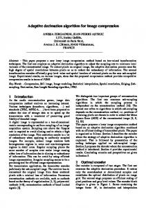
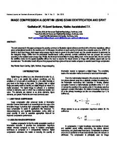
33 because of the variable-length coding employed. The DVQ code has a xed compression rate because of the xed-length coding of vector quantization. Figure 9 shows the original lenna image and Figures 10 and 11 show reconstructed images from the scalar DPCM algorithm and the DVQ algorithm with 256 codewords. Scalar DPCM yields a lower mean squared error than DVQ. However, as can be seen in these gures, the images are virtually indistinguishable from each other and the original. When the images of Figures 9 through 11 are magni ed, it can been seen that the DVQ algorithm results in some slight \blocky" distortion of edges, while the scalar DPCM algorithm maintains crisp edge reconstruction. Figures 12 and 13 show the di�erences created by subtracting Figures 10 and 11 from the original image, Figure 9. These di�erence images have been scaled and a constant has been added to enhance visibility. Figures 14 and 15 show images obtained with an error-prone channel (1 error per 1000 transmitted bits). As expected, the DVQ algorithm is signi cantly more robust to channel errors. The scalar DPCM simulation employed end-of-line synchronization codes, and, when a invalid code was encountered, the preceding line was copied to the remainder of the current line. Despite these compensatory measures, the channel errors produced dramatic distortions in the image, and occasionally, entire lines were missed when the end-of-line synchronization failed.
34
Figure 9: Lenna, original image
Figure 10: Reconstructed image using the scalar DPCM algorithm
35
Figure 11: Reconstructed image using the DVQ algorithm (256 codewords)
Figure 12: Di�erence between the reconstructed scalar DPCM image and the original image (enhanced)
36
Figure 13: Di�erence between the reconstructed DVQ image and the original image (enhanced)
Figure 14: Reconstructed image with an error-prone channel, scalar DPCM algorithm, ber = 1000
37
Figure 15: Reconstructed image with an error-prone channel, DVQ algorithm (256 codewords), ber = 1000
38
4.3 Codebook Entropies The entropies of the codebooks of sizes 128 and 256 were calculated for each image. The codebook entropy, H , for an image is N X H = ? pi log2 pi i=1
where
(4.1)
pi = PNni n
(4.2) j =1 j and N is the number of codewords in the codebook and ni is the number of times codeword i was used in the encoding of the image. As described in Section 2.1, vector quantization outputs xed-length codes for each tile. For the 128-codeword codebook, the code length is 7 bits/tile; for the 256-codeword codebook, the code length is 8 bits/tile. Table 5 shows the codebook entropies obtained from the encoding process. These entropies give the lower bound of the number of bits with which each tile could be encoded if Hu�man encoded was employed after VQ. For both codebooks, use of Hu�man coding can provide only an additional 1 bit/tile compression, on the average. The FSCL ANN training process produces codebooks with entropies that are close to the bit rate because the codebooks are constructed with equiprobable codewords. Consequently, Hu�man coding cannot contribute signi cant additional compression.
39
Table 5: Codebook entropies for DVQ Picture bird everest fruityy hall kittyy lenna mandril planey sceney sfy Average
Codebook Size 128 256 5.78 6.67 5.47 6.36 5.67 6.54 5.55 6.29 5.77 6.69 5.56 6.47 6.75 7.72 5.68 6.55 6.04 6.96 6.31 7.21 5.86 6.75
yImages used in the training of the codebooks.
CHAPTER V CONCLUSIONS AND FUTURE RESEARCH It has been shown that the di�erential vector quantization algorithm detailed in this paper achieves reasonable compression of monochrome images with tolerable amounts of distortion. When a 256 codeword codebook is used, the DVQ algorithm reduces an image to 25% of its original size. Since the vector quantization is performed on di�erence values, the blockiness associated with VQ is signi cantly reduced. Consequently, DVQ preserves edge features. Performance of the DVQ algorithm is comparable to scalar DPCM methods in terms of image quality and compression rate. The use of the FSCL ANN training procedure produces codebooks with codeword entropy close to the bit rate of the vector quantizer. Consequently, variable-length entropy encoding such as Hu�man coding, can be avoided. The xed-length VQ indices are robust to transmission errors; additionally, the codebook may be ordered to further reduce distortions due to errors. Thus, the DVQ algorithm has transmission error performance which is much better than that of the scalar DPCM system. The predictor and DPCM components of the DVQ algorithm were designed for simple hardware implementation. Consequently, the vector quantizer is the only 40
41 unit which requires complex processing. It is anticipated that the VQ operation may be implemented in hardware using an associative memory chip set [7]. Thus, a real-time hardware realization of the DVQ algorithm is possible. Such a hardware implementation is part of the future plans for this algorithm. Toward this end, the DVQ architecture will be adapted to process sampled NTSC composite color television signals which are only slightly di�erent from the monochrome images used to develop the algorithm. Additionally, some form of temporal prediction will be incorporated. This interframe prediction should provide additional compression and higher-quality output images. Finally, the vector quantizer will be made adaptive. It is expected that a FSCL ANN architecture will be used to train new codewords online to update the codebook as image statistics change.
References [1] A. K. Jain, Fundamentals of Digital Image Processing. Englewood Cli�s, NJ: Prentice Hall, 1989. [2] P. H. Ang, P. A. Ruetz, and D. Auld, \Video Compression Makes Big Gains," IEEE Spectrum, vol. 28, pp. 16{19, October 1991. [3] W. G. Hartz, R. E. Alexovich, and M. S. Neustadter, \Data Compression Techniques Applied to High Resolution High Frame Rate Video Technology," NASA Contractor Report 4263, Analex Corporation, Cleveland, Ohio, December 1989. Prepared for NASA Lewis Research Center under Contract NAS3-24564. [4] M. J. Shalkhauser and W. A. Whyte, Jr., \Digital CODEC for Real-Time Processing of Broadcast Quality Video Signals at 1.8 Bits/Pixel," Technical Report NASA TM-102325, National Aeronautics and Space Administration, Lewis Research Center, Cleveland, 1989. Prepared for Global Telecommunications Conference sponsored by IEEE, Dallas, Texas, Nov 27-30, 1989. [5] C. W. Rutledge, \Vector DPCM: Vector Predictive Coding of Color Images," in Proceedings of the IEEE Global Telecommunications Conference, pp. 1158{ 1164, September 1986. [6] R. M. Gray, \Vector Quantization," IEEE ASSP Magazine, vol. 1, pp. 4{29, April 1984. [7] A. K. Krishnamurthy, S. B. Bibyk, and S. C. Ahalt, \Video Data Compression Using Arti cial Neural Network Di�erential Vector Quantization," in Proceedings of the Second NASA Space Communications Technology Conference, (Cleveland, OH), pp. 95{101, November 1991. [8] S. C. Ahalt, P. Chen, and A. K. Krishnamurthy, \Performance Analysis of Two Image Vector Quantization Techniques," in Proceedings of the International Joint Conference on Neural Networks, vol. I, (Washington, D.C.), pp. 169{175, June 18{22, 1989. [9] Y. Linde, A. Buzo, and R. M. Gray, \An Algorithm for Vector Quantizer Design," IEEE Transactions on Communications, vol. COM-28, pp. 84{95, January 1980. [10] S. C. Ahalt, A. K. Krishnamurthy, P. Chen, and D. E. Melton, \Competitive Learning Algorithms for Vector Quantization," Neural Networks, vol. 3, pp. 277{290, 1990. 42
43 [11] A. K. Krishnamurthy, S. C. Ahalt, D. Melton, and P. Chen, \Neural Networks for Vector Quantization of Speech and Images," IEEE Journal on Selected Areas in Communications, vol. 8, pp. 1449{1457, October 1990.