Hindawi Publishing Corporation Mathematical Problems in Engineering Volume 2016, Article ID 6180758, 8 pages http://dx.doi.org/10.1155/2016/6180758
Research Article An ANN-GA Framework for Optimal Engine Modeling Khaldoun K. Tahboub,1 Mahmoud Barghash,1 Mazen Arafeh,1 and Osama Ghazal2 1
Industrial Engineering Department, The University of Jordan, Amman 11942, Jordan Mechanical and Industrial Engineering Department, Applied Science University, Amman, Jordan
2
Correspondence should be addressed to Mahmoud Barghash;
[email protected] Received 2 November 2015; Accepted 11 February 2016 Academic Editor: Hung-Yuan Chung Copyright © 2016 Khaldoun K. Tahboub et al. This is an open access article distributed under the Creative Commons Attribution License, which permits unrestricted use, distribution, and reproduction in any medium, provided the original work is properly cited. Internal combustion engines are a main power source for vehicles. Improving the engine power is important which involved optimizing combustion timing and quantity of fuel. Variable valve timing (VVT) can be used in this respect to increase peak torque and power. In this work Artificial Neural Network (ANN) is used to model the effect of the VVT on the power and genetic algorithm (GA) as an optimization technique to find the optimal power setting. The same proposed technique can be used to improve fuel economy or a balanced combination of both fuel and power. Based on the findings of this work, it was noticed that the VVT setting is more important at high speed. It was also noticed that optimal power can be obtained by changing the VVT settings as a function of speed. Also to reduce computational time in obtaining the optimal VVT setting, an ANN was successfully used to model the optimal setting as a function of speed.
1. Introduction Internal combustion engines have been a major power source throughout the history of ground vehicles. The two dominating combustion concepts, the Otto engine and the Diesel engine, were developed in the late 1800s. The introduction of electronic ignition and fuel injection systems in the 1980s have given the engineers far more capability of engine control than before. Since then, both fuel economy and emissions have improved, but still more progress can be expected in the future. One of the limitations in engine control development lies in the scarce online information about the controlled process, the combustion [1]. Variable valve timing (VVT) is used in spark ignition automotive engines to improve fuel economy, reduce NO𝑥 gases, and increase peak torque and power [2]. Valve control is one of the most important parameters for optimizing efficiency and emissions, permitting combustion engines to conform to future emission targets and standards. Thermodynamic conditions during the closed cycle (compression, combustion, and expansion) can be directly controlled by adjusting the intake valve opening (IVO) and intake valve closing (IVC) angle, which defines the total intake mass flow rate and the effective compression ratio of the engine [3].
Control of the intake valve provides optimal filling of the cylinder at all engine speeds. This natural supercharging, and the improved engine torque and power that accompany it, makes it possible to downsize engine capacity and thus reduce fuel consumption at all operating conditions [4]. Variable valve timing (VVT) relates to both the opening time and the duration of the valve’s open interval. Controlling valve timing can improve the torque curve, the brake power curve, or the indicator-power curve of a given engine. Variable valve timing can also be used to reduce the fuel consumption and, to a small extent, the engine emissions [5]. The adoption of a continuous variable valve timing (VVT) system is able to optimize engine torque and efficiency [6]. Genetic algorithm (GA) as an optimization technique is widely used for optimization of engineering problems. Many engineering design problems are very complex and therefore difficult to solve with conventional optimization techniques [7]. There are some studies in the literature about using GA for optimization of engine characteristics [8–11]. There is no guarantee that a GA will give an optimal solution or arrangement; there is only a guarantee that the solution will be near optimal in the light of the specific fitness function used in the evaluation of the many possible solutions generated. By near optimal, it is implied that a more optimal
2 solution may exist; however, the stochastic approach is by nature nondeterministic and therefore global optima cannot be guaranteed, and some hybrid techniques exist to combine “hill-climbing” deterministic approaches to stochastic GA approaches to determine the best solution to the accuracy required after the GA method has determined the best region of space to investigate. However, this refinement is not necessary in this study [12]. Artificial Neural Network (ANN) models may be used as an alternative way in engineering analysis and predictions. They are recently used also in engine optimization regarding engine operating parameters and emissions [13–16]. ANN models mimic somewhat the learning process of a human brain. They operate like a “black box” model, requiring no detailed information about the system. Instead, they learn the relationship between the input parameters and the controlled and uncontrolled variables by studying previously recorded data, similar to the way a nonlinear regression might perform. Another advantage of using ANNs is their ability to handle large and complex systems with many interrelated parameters. They seem simply to ignore excess data that are of minimal significance and concentrate instead on the more important inputs [12, 17]. Also the neural networks can be used in the form of an ensemble which highly adds to the accuracy of these ANNs [18]. Several methodologies for analysis and optimization of diesel engines including DoE [19], Support Vector Machine (SVM) [20], fuzzy modeling [21], particle swarm optimization [22], and specialized modeling software such as MATLAB [23] have been reported or can be used. In this work, different techniques are applied in the form of a multistage methodology. ANNs are used for engine modeling as a tool for optimization using GA. This GA is run for the purpose of determining the optimal power conditions at each speed. The ANN is used in reverse to dictate the optimal conditions according to speed.
2. Mathematical Background 2.1. Artificial Neural Networks. An Artificial Neural Network is based on the biological neural networks (nervous system) and is composed of “neurons” or “neurodes,” which are artificial nodes, processing elements, or “units.” A neural network is a mathematical model that is based on interconnection of the neurons and the strength of the connections (weights and biases) to model the majority of not all possible known functions. Neural networks in that respect are a generalized function that can be used to model complex relationships between inputs and outputs or to classify patterns in data. A schematic diagram of a typical multilayer feed-forward neural network architecture is shown in Figure 1(a). The network usually consists of an input layer, some hidden layers, and an output layer. In its simple form, each single neuron is connected to other neurons of a previous layer through adaptable synaptic weights. Knowledge is usually stored as a set of connection weights (presumably corresponding to synapse efficacy in biological neural systems). Figure 1(b) shows how information is processed through a single node.
Mathematical Problems in Engineering
···
···
Input layer
Output layer ··· Hidden layers
(a)
x1
Wi1
xj
Wij
xn
Win Weights
∑
Summation
𝛼
For the neuron i 𝛼i = f(Σnj=1 xj wij )
Activation
(b)
Figure 1: (a) The basic schematic of an Artificial Neural Network. (b) The basic information processing in a neural network unit [24].
The node receives weighted activation of other nodes through its incoming connections. First, these are added up (summation). The result is then passed through an activation function; the outcome is the activation of the node. For each of the outgoing connections, this activation value is multiplied with the specific weight and transferred to the next node [24]. Training of the neural network is done using back propagation where the error value and the local gradient of the error are used to estimate the new value of the weights and biases Δ𝑊𝑗𝑖 = 𝜂𝛿𝑗 (𝑛) 𝑦𝑖 (𝑛) ,
(1)
where 𝑊𝑗𝑖 is synaptic weight connecting the nodes, 𝜂 is learning rate, 𝛿𝑗 (𝑛) is the local gradient for the error in output neuron 𝑗 at iteration 𝑛, 𝑦𝑖 (𝑛) is the output of the network at neuron 𝑖 at iteration 𝑛, and 𝑛 is iteration number. Several types of neuron activation functions from logsig, tansig, and sigmoid functions were used as activation functions for the neural network. 2.2. Genetic Algorithm. Genetic algorithm (GA) is one type of evolutionary algorithms (EA) that mimics natural evolution as search heuristic to evaluate the global optimal in functions. This is opposed by the traditional optimization which may suffer from long time or local optimum. GA uses biological methods such as inheritance, mutation, selection, and crossover to generate solutions to optimization problems.
Mathematical Problems in Engineering Chromosome
3
1
Fitness
1
Stacked fitness
Selection
Population i
n
2
2
n
3
Random number
Selected parent
Crossover
Parent 1
1
1
1
0
0
0
0
0
1
0
1
0
1
1
1
0
0
0
1
1
0
0
1
0
1
0
Parent 2
0
0
0
1
1
0
0
1
1
0
0
0
1
1
1
0
0
0
1
1
1
0
0
0
1
0
Child 1
1
1
1
0
0
0
0
0
1
0
1
0
1
1
1
0
0
0
1
1
1
0
0
0
1
0
Child 2
0
0
0
1
1
0
0
1
1
0
0
0
1
1
1
0
0
0
1
1
0
0
1
0
1
0
Crossover point
Mutation point Mutation
1
1
1
0
0
0
0
0
1
0
1
0
1
1
1
0
0
0
1
1
1
0
0
0
1
0
1
1
1
0
0
0
0
0
1
0
1
0
0
1
1
0
0
0
1
1
1
0
0
0
1
0
Chromosome
1
n
2
Population i + 1
Figure 2: Graphical schematic of the genetic algorithm.
In a genetic algorithm, a population of candidate solutions (called individuals, creatures, or phenotypes) to an optimization problem is evolved toward better solutions. Each candidate solution has a set of properties (chromosomes or genotype) which can be mutated and altered; traditionally, solutions are represented in binary as strings of 0 s and 1 s, but other encodings are also possible. The evolution usually starts from a population of randomly generated individuals and happens in generations. In each generation, the fitness of every individual in the population is evaluated, the more fit individuals are stochastically selected from the current population, and each individual’s genome is modified (recombined and possibly randomly mutated) to form a new population. The new population is then used in the next iteration of the algorithm. Commonly, the algorithm terminates when either a maximum number of
generations have been produced or a satisfactory fitness level has been reached for the population. The basic GA is shown in Algorithm 1 and in Figure 2.
3. Methodology In this work we have followed the methodology shown in Figure 3. The engine data are obtained using suitable experimentation. The untrained ANN which is properly sized in terms of functions and neurons is trained for the experimentally obtained data. The result of this training process is trained ANN which can be used to predict the power of the considered engine at any given speed and valve timings. This ANN model is then used together with a genetic algorithm to evaluate the optimal engine parameters for a selected speed. Thus, the GA results are the optimal settings
4
Mathematical Problems in Engineering Table 1: Engine specifications. Begin 𝑡=0 Initialize Population 𝑃(𝑡) (random initialization) Evaluate fitness While (Generations < Total number) 𝑡=𝑡+1 Select Population for crossover Apply crossover Apply mutation End End
Bore Stroke Displacement volume Con rod length Compression ratio Intake valve diameter Exhaust valve diameter Maximum intake valve lift Maximum exhaust valve lift Intake valve opening Intake valve closing Exhaust valve opening Exhaust valve closing
Algorithm 1: Genetic algorithm. ANN untrained model
Engine data ANN training
The NSE can range from −∞ to 1. An efficiency of 1, that is, NSE = 1, corresponds to a perfect match between model and observations. An efficiency of 0 indicates that the model predictions are as accurate as the mean of the observed data. An efficiency less than 0, that is, −∞ < 𝐸 < 0, implies that the observed mean is a better predictor than the model. The Nash-Sutcliffe model efficiency coefficient (NSE) is commonly used to assess the predictive power of hydrological discharge models. However, it can also be used to quantitatively describe the accuracy of model outputs in other applications such as the one in this research [25].
ANN model
Select speed
X Y Speed Optimal engine parameters
Genetic algorithm
Optimal engine parameters
4. Engine and Experimental Practice
ANN untrained model
ANN training
For the purpose of analyzing the engine characteristics the dimensions were considered with a specially designed program used to predict the gas flows, combustion, and overall performance of internal combustion engines. Engine speed was varied between 1000 and 6000 rpm. Ignition was taken 10∘ bTDC. The specifications for the engine are in Table 1.
ANN optimal model
Figure 3: Proposed optimization methodology for SI engine timing settings.
for each engine speed. The data (speed versus optimal engine parameters) are then used to train the final ANN model. The validation of the results is done using visual inspection, Root Square Mean Error (RSME), that is, 2
∑𝑛 (𝑋obs,𝑖 − 𝑋model,𝑖 ) , RSME = √ 𝑖=1 𝑛
(2)
and the Nash-Sutcliffe model efficiency coefficient (NSE), that is, 2
NSE = 1 −
∑𝑛𝑖=1 (𝑋obs,𝑖 − 𝑋model,𝑖 ) ∑𝑛𝑖=1
(𝑋obs,𝑖 − 𝑋obs )
83 mm 80 mm 0.4328 liters 129.8 mm 10.5 : 1 30 mm 25 mm 9.5 mm 9.5 21∘ 75∘ 68∘ 32∘
=1−
MSE . 𝜎2
(3)
5. Results and Discussion The initial step is to train the untrained ANN for the experimentally obtained engine data (see Section 5.1). GA is used to select the optimal VVT settings for each speed (Section 5.2). The data (speed versus optimal engine parameters) are then used to train the final ANN model (Section 5.3). 5.1. Training Accuracy of the ANN. ANN of four layers and three neurons per layer is trained for the experimental engine data. Figure 4 shows the ANN power prediction versus the actual values. ANN results fall well within 5% prediction error. The Root Mean Square Error (RMSE) for the model is 0.414. Thus one can conclude that ANN can predict the power of the engine accurately. The Nash-Sutcliffe coefficient 𝐸 for the results is 0.995 (close to 1). Thus the ANN prediction is very close to the practical results.
5
25
25.00 Optimal and nonoptimal break power (kW)
ANN predicted break power (kW)
Mathematical Problems in Engineering
20 15 10 5 0 0.00
5.00
10.00 15.00 Actual break power (kW)
20.00
25.00
Optimal break power (kW)
15.00 10.00
Power spread
5.00 0.00 0
Figure 4: ANN prediction of engine power versus actual break power. 24 22 20 18 16 14 12 10 8 6 4 1000
20.00
1000
2000 3000 4000 5000 Engine speed (rpm)
6000
7000
Break power Optimal break power
Figure 6: Power spread drawn for all the experimental VVT settings at different engine speeds in addition to optimal power (highest).
2000
3000 4000 5000 Engine speed (rpm)
6000
7000
Figure 5: Optimal power in KW as predicted by NN-GA framework versus speed in RPM.
5.2. Optimal Break Power and Break Power Spread. The genetic algorithm is then used to obtain optimal power VVT setting at each speed. 150 generations are used to achieve the results. Figure 5 shows the obtained optimal power versus engine speed. As expected the power increases with speed, but the curve is slightly quadratic. Within the range 2500– 6000 rpm we can approximate the curve with a linear line with little information lost in that respect. The break power generally increases as the speed increases. As the speed increases friction power increases and the volume of air swept in the engine is reduced; thus the curves tend to increase but with less slope to reflect these two important perspectives. Figure 6 shows the optimal and nonoptimal power in one curve versus engine speed. The 𝑥-points are the break power at any parameter settings. One important criterion is noticed from the curve which is the importance of the setting is variable with speed. At a speed of 1000 rpm, there is ample time for enough air to flow in and thus the parameter settings are not as important as those for the higher speed where bad setting can lead to unignorable reduction in break power. 5.3. GA Optimization of Break Power at Each Engine Speed. Figure 7 shows the VVT optimal setting as a function of speed. The optimal oven valve intake has two main modes; at low speed the optimal setting increases as speed increases; thus we need more open valve intake time to achieve the
optimal power. But the value of this parameter is stabilized at its maximum setting. The intake valve closing at low speeds is not of great importance; thus it is a low setting, but as the speed gets higher we need more time for the valve closing to achieve optimal power. The exhaust valve opening is set at a high initial value at low speed while at higher speeds, it will be fluctuating around its average setting, while exhaust valve closing is set at its highest time to achieve optimal power. The RMS error for the predictions is 0.0274 for the intake valve opening, 0.43 for the intake valve closing, 1.82 for the exhaust valve closing, 0.793 for the exhaust valve opening, and 0 for the exhaust valve closing. The latter is the highest prediction error because it can change with a higher range without affecting the optimal power. The Nash-Sutcliffe coefficient is 0.99993 for the intake valve opening, 0.993 for the intake valve closing, 0.701 for the exhaust valve opening, and 1 for the exhaust valve closing. 5.4. Optimal ANN Model for VVT . The final stage of this work is to build an ANN model for predicting the optimal VVT settings at each speed. The ANN model is trained for the optimal settings at each speed. The ANN is trained to give the optimal VVT settings given the engine speed as the input. This model can be programmed using a suitable microcontroller or microprocessor and when measuring the engine speed it can estimate or predict the VVT and applies these settings on the engine. The predicted model is shown in Figure 8. Figure 9 shows a comparison between the power obtained using the recommended settings and the actual optimal power. It shows that the achieved model predicts the right optimal power successfully. The RMS for the power prediction is 0.058 which shows the excellent prediction of the system proposed. The Nash-Sutcliffe coefficient is 0.99991 for the data.
6. Conclusions This work utilized ANN to model the break power and GA is used to obtain the optimal setting at each speed. Another
6
Mathematical Problems in Engineering 26
60
Intake valve closing (deg)
Intake valve opening (deg)
24 22 20 18 16
55
50
45
14 40
12 500
2500 4500 Engine speed (rpm)
6500
500
6500
Predicted Actual
Predicted Actual 54
50
52
45 Exhaust valve closing (deg)
Exhaust valve opening (deg)
2500 4500 Engine speed (rpm)
50 48 46 44
40 35 30 25
42 40 500
2500
4500
6500
20 500
2500 4500 Engine speed (rpm)
Engine speed (rpm) Predicted Actual
6500
Predicted Actual
Figure 7: Optimal engine parameters as predicted by the GA-NN framework versus speed.
ANN model is used to predict the optimal VVT settings at each speed. We can conclude the following: (1) The ANN model can be successfully used to predict engine power using the VVT settings and the speed well within 5% error margin. (2) Through using GA, optimal valve settings at low speeds (1000) are the intake valve opening low (13), intake valve closing low (42), exhaust valve opening high (52), and exhaust valve closing high (30). At intermediate speeds (3000) optimal valve settings are intake valve opening high (25), intake valve closing low (42), exhaust valve opening low (44), and exhaust valve closing high (30). At high speeds (6000) the optimal valve settings are intake valve opening high (25), intake valve closing high (57), exhaust valve opening low (44), and exhaust valve closing high (30).
(3) The ANN model is used to successfully model the optimal GA prediction for the VVT settings over speeds from 1000 to 6000 rpm to an accuracy less than 2%. (4) It was noticed that open valve intake is optimal as low at low speed but is optimal at high value when the engine is at high speed. (5) The intake valve closing is optimal as low at low speeds but we need to increase it gradually as speed is increased. (6) The exhaust valve opening is optimal as high when the speed is low but it fluctuates around a certain average value at higher speed. (7) The exhaust valve closing is optimal at high value at all engine speeds. (8) Finally, RMSE and NSE measures were used to evaluate model accuracy and prediction efficiency. A NSE
Mathematical Problems in Engineering
7 −0.0047708 −12.8783
X 1 1 + e−x
+ 6.8265
X Optimal intake valve opening (deg)
+ 25.0092
−0.001711 [−26.1525]
Speed (rpm)
X +
1 1 + e−x
[9.6597]
X + [67.7546]
Optimal intake valve closing (deg)
0.096583 [−8.9917] X +
1 1 + e−x
[−144.6528]
X +
Optimal exhaust valve opening (deg)
[52.9204]
[−0.00022631] [−76.6177] X + [0.1616]
1 1 + e−x
X +
Optimal power
[41.5099]
Predicted optimal break power using ANN recommended settings at specified engine speeds
Figure 8: The optimal structure for the NN predicting the optimal engine parameters using speed.
25 20 15 10 5 0 0
5 10 15 20 Optimal break power at specified engine speeds
25
Figure 9: Validation of the final ANN; predicted optimal power versus actual optimal power.
8
Mathematical Problems in Engineering of higher than 0.99 was achieved in both ANNs which reflects the high prediction accuracy of these models in predicting optimal valve settings for maximum engine power output.
Disclosure This work was partially executed during a sabbatical leave of the first author.
Competing Interests The authors declare that there are no competing interests regarding the publication of this paper.
References [1] S. Larsson and I. Andersson, “Self-optimising control of an SIengine using a torque sensor,” Control Engineering Practice, vol. 16, no. 5, pp. 505–514, 2008. [2] O. H. Ghazal, Y. S. Najjar, and K. J. AL-Khishali, “Effect of inlet valve variable timing in the spark ignition engine on achieving greener transport,” International Journal of Mechanical, Aerospace, Industrial, Mechatronic and Manufacturing Engineering, vol. 5, no. 11, pp. 2543–2547, 2011. [3] J. Benajes, S. Molina, J. Mart´ın, and R. Novella, “Effect of advancing the closing angle of the intake valves on diffusioncontrolled combustion in a HD diesel engine,” Applied Thermal Engineering, vol. 29, no. 10, pp. 1947–1954, 2009. [4] M. G¨olc¨u, Y. Sekmen, P. Erduranlı, and M. S. Salman, “Artificial neural-network based modeling of variable valve-timing in a spark-ignition engine,” Applied Energy, vol. 81, no. 2, pp. 187– 197, 2005. [5] S. Nagumo and S. Hara, “Study of fuel economy improvement through control of intake valve closing timing: cause of combustion deterioration and improvement,” JSAE Review, vol. 16, no. 1, pp. 13–19, 1995. [6] R. Fiorenza, M. Pirelli, E. Torella et al., “Variable swirl and internal EGR by VVT application on small displacement 2 valve SI engines: an intelligent technology combination,” in Proceedings of the FISITA World Automotive Congress, May 2004. [7] M. Gen and R. Cheng, Genetic Algorithms and Engineering Design, John Wiley & Sons, London, UK, 1997. [8] A. Homaifar, H. Y. Lai, and E. McCormick, “System optimization of turbofan engines using genetic algorithms,” Applied Mathematical Modelling, vol. 18, no. 2, pp. 72–83, 1994. [9] D. A. Manolas, “Operation optimisation of an industrial cogeneration system by a genetic algorithm,” Energy Conversion and Management, vol. 38, pp. 15–17, 1997. [10] Z. Hao, C. Kefa, and M. Jianbo, “Combining neural network and genetic algorithms to optimize low NO𝑥 pulverized coal combustion,” Fuel, vol. 80, no. 15, pp. 2163–2169, 2001. [11] S. Ogaji, S. Sampath, R. Singh, and D. Probert, “Novel approach for improving power-plant availability using advanced engine diagnostics,” Applied Energy, vol. 72, no. 1, pp. 389–407, 2002. [12] U. Kesgin, “Genetic algorithm and artificial neural network for engine optimisation of efficiency and NOx emission,” Fuel, vol. 83, no. 7-8, pp. 885–895, 2004.
[13] D. Yuanwang, Z. Meilin, X. Dong, and C. Xiaobei, “An analysis for effect of cetane number on exhaust emissions from engine with the neural network,” Fuel, vol. 81, no. 15, pp. 1963–1970, 2002. [14] H. C. Krijnsen, J. C. M. van Leeuwen, R. Bakker, C. M. van den Bleek, and H. P. A. Calis, “Optimum NO𝑥 abatement in diesel exhaust using inferential feedforward reductant control,” Fuel, vol. 80, no. 7, pp. 1001–1008, 2001. [15] A. Dur´an, A. De Lucas, M. Carmona, and R. Ballesteros, “Simulation of atmospheric PAH emissions from diesel engines,” Chemosphere, vol. 44, no. 5, pp. 921–924, 2001. [16] A. De Lucas, “Modelling diesel particulate emissions with neural networks,” Fuel, vol. 80, pp. 539–548, 2001. [17] S. A. Kalogirou, “Applications of artificial neural networks in energy systems: a review,” Energy Conversion and Management, vol. 40, no. 10, pp. 1073–1087, 1999. [18] M. Barghash, “An effective and novel neural network ensemble for shift pattern detection in control charts,” Computational Intelligence and Neuroscience, vol. 2015, Article ID 939248, 9 pages, 2015. [19] G. Di Blasio, M. Viscardi, and C. Beatrice, “DoE method for operating parameter optimization of a dual-fuel bioethanol/diesel light duty engine,” Journal of Fuels, vol. 2015, Article ID 674705, 14 pages, 2015. [20] F. Shi, J. Chen, Y. Xu, and H. R. Karimi, “Optimization of biodiesel injection parameters based on support vector machine,” Mathematical Problems in Engineering, vol. 2013, Article ID 893084, 8 pages, 2013. [21] S. Simani and M. Bonf`e, “Fuzzy modelling and control of the air system of a diesel engine,” Advances in Fuzzy Systems, vol. 2009, Article ID 450259, 14 pages, 2009. [22] B. Wahono and H. Ogai, “Combustion model and control parameter optimization methods for single cylinder diesel engine,” Journal of Optimization, vol. 2014, Article ID 135163, 9 pages, 2014. [23] K. Chan, A. Ordys, K. Volkov, and O. Duran, “Comparison of engine simulation software for development of control system,” Modelling and Simulation in Engineering, vol. 2013, Article ID 401643, 21 pages, 2013. [24] S. A. Kalogirou, “Artificial intelligence for the modeling and control of combustion processes: a review,” Progress in Energy and Combustion Science, vol. 29, no. 6, pp. 515–566, 2003. [25] H. V. Gupta, H. Kling, K. K. Yilmaz, and G. F. Martinez, “Decomposition of the mean squared error and NSE performance criteria: implications for improving hydrological modelling,” Journal of Hydrology, vol. 377, no. 1-2, pp. 80–91, 2009.
Advances in
Operations Research Hindawi Publishing Corporation http://www.hindawi.com
Volume 2014
Advances in
Decision Sciences Hindawi Publishing Corporation http://www.hindawi.com
Volume 2014
Journal of
Applied Mathematics
Algebra
Hindawi Publishing Corporation http://www.hindawi.com
Hindawi Publishing Corporation http://www.hindawi.com
Volume 2014
Journal of
Probability and Statistics Volume 2014
The Scientific World Journal Hindawi Publishing Corporation http://www.hindawi.com
Hindawi Publishing Corporation http://www.hindawi.com
Volume 2014
International Journal of
Differential Equations Hindawi Publishing Corporation http://www.hindawi.com
Volume 2014
Volume 2014
Submit your manuscripts at http://www.hindawi.com International Journal of
Advances in
Combinatorics Hindawi Publishing Corporation http://www.hindawi.com
Mathematical Physics Hindawi Publishing Corporation http://www.hindawi.com
Volume 2014
Journal of
Complex Analysis Hindawi Publishing Corporation http://www.hindawi.com
Volume 2014
International Journal of Mathematics and Mathematical Sciences
Mathematical Problems in Engineering
Journal of
Mathematics Hindawi Publishing Corporation http://www.hindawi.com
Volume 2014
Hindawi Publishing Corporation http://www.hindawi.com
Volume 2014
Volume 2014
Hindawi Publishing Corporation http://www.hindawi.com
Volume 2014
Discrete Mathematics
Journal of
Volume 2014
Hindawi Publishing Corporation http://www.hindawi.com
Discrete Dynamics in Nature and Society
Journal of
Function Spaces Hindawi Publishing Corporation http://www.hindawi.com
Abstract and Applied Analysis
Volume 2014
Hindawi Publishing Corporation http://www.hindawi.com
Volume 2014
Hindawi Publishing Corporation http://www.hindawi.com
Volume 2014
International Journal of
Journal of
Stochastic Analysis
Optimization
Hindawi Publishing Corporation http://www.hindawi.com
Hindawi Publishing Corporation http://www.hindawi.com
Volume 2014
Volume 2014