Graduate School of Information Science, Nara Institute of Science and Technology, Nara, JAPAN ...... Accelerated Algorithm for High Quality Rendering of Vi- sual Hulls,â In ... BS degrees in computer science from the National Institute of.
10
JOURNAL OF MULTIMEDIA, VOL. 2, NO. 1, FEBRUARY 2007 1
An Assignment Scheme to Control Multiple Pan/Tilt Cameras for 3D Video Sofiane Yous, Norimichi Ukita, and Masatsugu Kidode Graduate School of Information Science, Nara Institute of Science and Technology, Nara, JAPAN Email: {yous-s, ukita, kidode}@is.naist.jp
Abstract— This paper presents an assignment scheme to control multiple Pan/Tilt (PT) cameras for 3D video of a moving object. The system combines static wide field of view (FOV) cameras and active Pan/Tilt (PT) cameras with narrow FOV within a networked platform. We consider the general case where the active cameras have as high resolution as they can capture only partial views of the object. The major issue is the automatic assignment of each active camera to an appropriate part of the object in order to get high-resolution images of the whole object. We propose an assignment scheme based on the analysis of a coarse 3D shape produced in a preprocessing step based on the wide-FOV images. For each high-resolution camera, we evaluate the visibility toward the different parts of the shape, corresponding to different orientations of the camera and with respect to its FOV. Then, we assign each camera to one orientation in order to get high visibility of the whole object. The continuously captured images are saved to be used offline in the reconstruction of the object. For a temporal extension of this scheme, we involve, in addition to the visibility analysis, the last camera orientation as an additional constraint. This allows smooth and optimized camera movements. Index Terms— active camera control, 3D video, camera assignment, shape analysis.
I. I NTRODUCTION High-resolution images are a requirement for highresolution visualization and 3D reconstruction applications. For texture mapping [23] and shape refinement [22], priority is given to closer and accessible (without occlusion) viewpoints and with adequate angles of view [11], [12]. An example of these applications is 3D video system. Several systems have been proposed, such as (Fig. 1), [1], [5], [6], [7], [8], and [9]. These systems focus on capturing images of an acting human body and use a distributed static camera system for a real-time synchronized observation. While [6], [1], and [9] generate the final video offline, [4], [7], [8], and [10] employ a volume intersection method on a PC cluster in order to achieve a full 3D shape reconstruction in real time. A static camera system requires a continuous coverage of the entire observable area. This prevents the resolution of the cameras to be increased without affecting the coverage of the scene. To overcome this limitation, we have been designing a 3D video based on an active camera This paper is based on “Multiple Active Camera Assignment for High Fidelity 3D Video,” by S. Yous, N. Ukita, and M. Kidode, which appeared In Proceedings IEEE International Conference on Computer c 2006 IEEE. Vision Systems (ICVS) , New York, USA, January 2006.
© 2007 ACADEMY PUBLISHER
Cameras
Kimono lady
Figure 1. 3D video environment.
system. With such a system, the area to be covered is the one occupied by the moving object and hence, it is unnecessary to continuously observe the entire scene. Thus, it becomes possible to increase the resolution of the camera with more freedom. The proposed system combines stationary cameras having wide fields of view and active Pan/Tilt (PT) cameras with narrow FOV (high resolution). The sparse distribution of the active PT wide-FOV cameras does not allow the coverage of the entire scene. Thus it is necessary to control these cameras to gaze the object. The wide-FOV cameras, which can cover the entire scene with low resolution, are required to provide the necessary information about the object to steer the narrow-FOV cameras. We consider the general case where the narrow-FOV cameras can capture only partial views of the object, but with high resolution. In such situations, a camera can have different visibility to different parts of the same object following its 3D shape, as shown in Fig.2. From this figure, we can notice that the camera system configuration needs to be adjusted depending on the position and the posture of the target. If we consider the texture mapping or the refinement of the reconstructed Target
Fied of view of the camera
(a)
Camera1
Camera1
Camera2
Camera2
(b)
Figure 2. The configuration of the two cameras differs from (a) to (b), depending of the posture of the target.
JOURNAL OF MULTIMEDIA, VOL. 2, NO. 1, FEBRUARY 2007
Online processing Image capture (wide-FOV cameras)
Image capture (narrow-FOV cameras)
3D shape reconstruction
Assignment (narrow-FOV cameras)
Offline processing
Final 3D video building
Figure 3. System operation.
3D shape, the camera is more useful in some regions than others. Therefore, we propose a multiple active PT camera assignment to assign each camera to one part in order to provide high-resolution images and with high visibility of the whole object. The depth, occlusion, and angle of incidence constraints are taken into account in this assignment scheme. The wide-FOV cameras are charged to provide global information about the position and posture of the target, necessary for the assignment of wide-FOV cameras. The rest of this paper is organized as follows: Section II gives an overview of the active camera system. Section III describes the camera assignment scheme. We detail the different steps of this scheme in the sections IV, V, VI, and VII, and evaluate the overall scheme in section VIII. We conclude this paper by a summary and future work in section IX. II. S YSTEM OVERVIEW The proposed system consists of an offline and an online subsystems. In the offline processing side, where the processing time is not very important, sophisticated 3D reconstruction algorithms, such as deformable mesh model [4] and space carving [22], are employed to produce the final 3D video using the images captured online. Basically, high-resolution images are used for this reconstruction. However, wide-FOV images are useful to recover and reconstruct the non-covered areas when the narrow-FOV cameras do not cover the entire object. As an online processing, the cameras are controlled following the position and posture of the target. A. System Operation Fig. 3 summarizes how the captured images flow through the different steps of the system. In the online processing, the images are captured continuously by all cameras, regardless of their types, and saved or transmitted to the offline processing. The images provided by the wide-FOV cameras are transmitted to the reconstruction process to produce a coarse shape of the object. This will guarantee the full reconstruction since these cameras have full views of the target. The high-resolution cameras are steered not only to follow the motion of the object, but rather, to be assigned to the different parts of the object in order to get highresolution images of the whole. The high-resolution cameras, contrary to those with wide FOV, lack global information about the object. These information are provided © 2007 ACADEMY PUBLISHER
11
through a coarse reconstruction of the target shape. Based on the analysis of this shape, each camera is assigned to one appropriate part. B. Assumptions So far, a general description of the proposed active camera system has been given. We focus on the assignment of high-resolution active cameras. The other parts of the system will not be covered here. The input of the assignment process is the reconstructed shape of the object. Based on the analysis of this shape, each camera is assigned to the most appropriate part of the object. The assignment scheme we propose estimates the camera configuration at time t + 1 based on a shape reconstructed at time t. If the object motion is so fast and the 3D shape reconstruction, camera assignment, and camera movement are not fast enough, the assignment will not achieve what it was designed for. Therefore, we assume that the object motion is relatively slow. One solution to avoid this problem in general cases, is to do not consider the full FOV for the narrow-FOV cameras. The difference will be set as a security margin to avoid that the region to which the camera is assigned goes out of the real FOV. Also, the assignment process, in addition to the 3D reconstruction and the camera movement, should be as fast as possible. III. M ULTIPLE ACTIVE C AMERA A SSIGNMENT Our goal is to control the active wide-FOV cameras in order to provide high resolution images for 3D reconstruction. The quality of the reconstruction is related to the photometric consistency of the produced shape. The 3D reconstruction methods start by reconstructing the Visual Hull (VH) of the observed object. Using a set of images taken from different viewpoints, the VH is refined based on photometric consistency criteria. The quality of a reconstructed 3D shape is measured by how the shape is photometrically-consistent. The photometric consistency is related to three main factors: Occlusion, angle of incidence, and depth. This is the fact that the photometric consistency is directly related to the re-projection error which is inversely proportional to the projection area on a texture image, as reported in [11] and [12]. The projection area is related to the angle of incidence and the distance between the camera and the surface patch in question. That is, a surface that is far or viewed at an oblique angle from all the cameras will have only few pixels projected to it. However, the surface which is visible, parallel to the image plane and close to a camera will have more pixels that project to it. On the other hand, it is clear that the more the points that project to a given surface, the better it is reconstructed (see [11] and [12] for more details). Starting from this, the multiple active camera assignment scheme should consider this photometric consistency in assigning each active PT camera to a specific orientation toward the object. In other words, the goal is the automatic assignment of each narrow-FOV camera to an appropriate part of the target in order to get
12
JOURNAL OF MULTIMEDIA, VOL. 2, NO. 1, FEBRUARY 2007
3D surface
Facets
Projection to the camera image planes
Vertices
Step 1
Windowing Step 2 Visibility evaluation
Figure 4. Input data : 3D mesh surface. Global assignment
high-resolution images of the whole object based on the photometric consistency requirements. The input is the 3D shape of the object in the form of a mesh surface O(V, F ); V and F are, respectively, the vertices and facets sets (Fig.4). Each facet is defined as a sequence of ordered vertices wherewith, the outward normal vector can be computed. In the rest of this chapter, we adopt the following notations: c ∈ {1..N }: The N PT cameras of our system. f ∈ {1..M }: The M facets composing the 3D mesh surface. − n→ f : The unit outward normal vector of a facet f . oc : The optical center of camera c. tf : The centroid of facet f . A. Assignment Constraints Based on the photometric consistency requirements, we summarize the constraints that should drive the assignment process as follows: 1) Angle of incidence constraint: for one camera, only the facets whose outward faces are oriented to the camera are taken into account. To meet this condition, a facet must have a negative dot product between its outward normal vector and the vector associated to the optical center of the camera and the centroid of the facet, as follows: −−→ f visible f rom c ⇒ (− n→ (1) f · oc tf ) < 0 Furthermore, if both vectors are normalized, then the dot product can quantify the visibility (details in V). That is, the higher the absolute value of the dot product, the better the visibility. 2) Occlusion constraint: for one camera, only nonoccluded facets are considered. The set of facets V (c) meeting the angle of incidence condition and not occluded with respect of a camera c, are provided by the related depth image Dc . We associate an index image Ic having as attributes the indices (identifiers) of these facets. V (c) can be defined such that: j ∈ V (c) ⇔ ∃x,y Ic (x, y) = j
(2)
3) FOV constraint: only the region observed within the FOV of a given camera is taken into account while the whole surface is projected onto the image plane. 4) Depth constraint: the camera-object distance is taken into account in the assignment process. That © 2007 ACADEMY PUBLISHER
Step 3
Figure 5. Flowchart of the assignment scheme.
is, a camera should have more chances to be assigned to closer regions. 5) 3D reconstruction constraint: this constraint requires us to have at least two views toward each surface point in order to allow the refinement of 3D shape .(e.g. shape by space carving [22]).
B. Overview of the Assignment Scheme The camera assignment is realized by analyzing the 3D surface and seeks for the best camera set-up that allows the best visibility of all object parts, knowing that: • • •
A camera can have a large number of possible orientations. A camera contributes in the visibility of the whole 3D surface depending of its orientation. For one orientation, the camera contributes in the global visibility through the subset of facets visible within its FOV.
In order to reduce the possibilities of one camera orientations, we introduce the windowing scheme that will be presented in section IV. As a result of this scheme, the facets concerned by each orientation are selected and involved in the evaluation of the orientation. For this evaluation, visibility quantification is introduced in section V. As for the global assignment, it is the subject of section VI. The proposed algorithm can be summarized in three steps (Fig.5): 1) Step1: the 3D shape is projected onto the panoramic 1 planes of all cameras as shown in the upper part of Fig.6. 2) Step2: the orientations to the object regions are evaluated for each camera with respect to its FOV. In the panoramic image, each orientation corresponds to a window determined by the camera FOV. For a given window (orientation), the evaluation concerns the visibility to the corresponding 3D surface region (lower part of Fig.6). 1 The panoramic plane of a given camera is a reference plane corresponding to a chosen camera orientation(e.g., (pan, tilt) = (0, 0)). All the images of this chapter correspond to this plane. See [21] for details.
JOURNAL OF MULTIMEDIA, VOL. 2, NO. 1, FEBRUARY 2007
Step 1
13
The bounded object region in depth image
Panoramic planes Windows
Object projection
The bounded remaining object region in depth image
Step 2
(a)
(b)
(c)
Figure 7. Windowing scheme: From (a) to (b) a flood filling is applied, and an adjustment is applied to get (c). The top cycle corresponds to the first windowing iteration for a given camera. The missing part in the depth image of the bottom cycle was windowed and deleted in previous iterations. Figure 6. The first two steps of the proposed algorithm.
3) Step3: the best assignment configuration between the cameras and the windows that maximizes the global visibility is sought. IV. W INDOWING S CHEME The goal of the windowing scheme is twofold: 1) select from the huge possible orientations, a small set that cover the object view based on the FOV constraints, and 2) select for each orientation the set of facets that satisfy the angle of incidence and occlusion constraints. In addition, we consider the fact that under self-occlusion conditions, a camera can have a view of regions with discontinuous depths within the same FOV. We impose the the connectivity as an additional constraint to assign a camera to one region with continuous depth. To achieve such a goal, we proceed with gradually splitting the depth image into several windows. After setting a window to the offset of the bounding rectangle of the object region in depth image, a flood-filling is applied to the region of interest defined by the window in order to extract one connected region. Then, the window position is repeatedly readjusted by shifting in order for the window to fit the best with the connected region. For each new position, the flood-filling is reapplied to find the new limits of the connected region. Finally, this region is withdrawn from the depth image and used as a mask for the index image in order to select the facets to be involved in the visibility evaluation. Let us denote by wkc |k=1..K the K resulted windows, and (xk , yk ) their respective off-set addresses with respect to the depth image. If a given point has (x, y) as coordinates in the window wkc , then its coordinates in the original image are (x + xk , y + y k ). If this point belongs to the connected region, then wkc (x, y) > 0 (The point (x, y) in the window wkc is strictly positive). The set of facets V (c) is splitted into V (c, k)|k=1..K © 2007 ACADEMY PUBLISHER
such that: S k V (c, k) = V (c) ∧ f ∈ V (c, k) c⇔ wk (x, y) > 0 ∧ ∃ x,y Ic (xk + x, yk + y) = f
(3)
The proposed algorithm is summarized in what follows (Fig.7): 1) Define the bounding rectangle of the object region in the depth image if it is the first iteration or of the remaining regions of the object if not. The bounded region will be set as the region of interest (ROI) of the depth image, as shown in Fig.7-a. 2) Set a window to the offset of the ROI (Fig.7-a). 3) Repeat: • Apply a flood-filling starting from the top-left seed point of the object region in the window, as shown in Fig.7-b. • Shift the window along the bounded region in order to bring the outer contours of the connected region to the borders of the window. If we consider the top window of Fig.7-b, the window has to be shifted in the right direction. After applying the flood-filling, we get the top window of Fig.7-c. Until the top and left borders of the window meet the external contour of the connected component. If it is the last horizontal window, we consider the right border of the window instead of the left. Similarly, we consider the bottom border instead of the top if it is the last vertical window (Fig.7-c). 4) Save the window and delete the area corresponding to the connected component from the depth image. This window will serve as a mask to the index image in order to select the corresponding facets set.
14
JOURNAL OF MULTIMEDIA, VOL. 2, NO. 1, FEBRUARY 2007
5) If the depth image is not empty, then goto 1. At the end of this process, a set of windows for each camera is obtained. Each camera orientation is evaluated using the selected facets, as explained in the following section.
•
ˆ (c, k) = M INf ∈V (c,k) (D (c, f )) D
V. V ISIBILITY Q UANTIFICATION The possible orientations for each camera been defined, the next step will be the evaluation of each of them based on the visibility analysis. Based on the constraints derived from the photometric consistency requirements, we quantify the visibility at three levels: Facet-wise, local, and global. A. Facet-wise Visibility Quantification The facet-wise visibility is the direct application of the angle of incidence constraint and concerns the visibility of a given facet from a given camera. It can be expressed by the absolute value of the dot product between the unit normal vector of the facet in question in one side and the normalized vector connecting the optical center of the camera and the centroid of the facet in the other side. If the unit vector, corresponding to the optical ray of a camera ci toward tj , is: −→
oc tf → rc,f = −→
oc tf Then, the facet-wise visibility is given by: → → F (c, f ) = rc,f · nf
•
where D (c, f ) denotes the depth of f with respect to c. S¯ (c, k), the area of the 3D surface related to the window wkc of a camera c such that: X S¯ (c, k) = S (f ) f ∈V (c,k)
where S (j) denotes the surface area of a facet fj in the 3D space. The local visibility of a window wkc from a camera c is given by: ˆ (c, k) D L(c, k) = ¯ . S (c, k)
X f ∈V (c,k)
F (c, f ) .S (f ) D (c, f )
(5)
For a set of facets V (c, k), the local visibility is the normalization of the sum of the scaled facet-wise visibility of these facets. The scale is the ratio between the 3D surface area of the facet and the depth of its centroid with respect to the camera in question. As for the normalizing factor, it is the ratio between the minimum depth of the 3D surface and its 3D area. C. Global Visibility Quantification
(4)
B. Local Visibility Quantification For one camera, the local visibility level concerns the visibility toward each of its windows selected by the windowing scheme. For a given window, it involves the facet-wise visibility of all facets related to the window. The formulation of the local visibility is very important, since it is on which the global assignment is based. The straightforward way to quantify the local visibility is to sum the facet-wise visibility of the corresponding facets. Though simple, this solution has the following disadvantages: 1) A narrow region made of tiny facets is given similar evaluation as a wide region with large facets if the two regions have a similar number of facets. 2) One region is given the same evaluation whatever its distance from the camera. In order to overcome these disadvantages, the proposed formulation should: 1) Respect the aforementioned depth constraint. 2) Involve the facet area. That is, the contribution of each facet in the local visibility should be proportional to its surface area. 3) Be normalized. Let us denote by: © 2007 ACADEMY PUBLISHER
ˆ (c, k), the depth of the nearest point of the 3D D surface within a window wkc with respect to a camera c such that:
The purpose of the assignment process is to maximize the global visibility of the 3D surface. After the system is set to a given configuration, this global visibility can be expressed by averaging the local visibility of all cameras. Let us assimilate the assignment scheme by a function A that associates to a camera c the assigned window wqc . A˙ is the set of couples (c, q) such that: A˙ = {(c, q)/A : c → Assignedwqc } Then the global visibility is given by: G=
1 N
X
L (i, j)
(6)
(i,j)∈A˙
VI. G LOBAL A SSIGNMENT S CHEME After having addressed the windowing and visibility quantification issues, we are now able to establish a global assignment scheme. The purpose is to direct each camera toward a specific part of the object in order to get a high visibility of the whole object. This can be reduced to select for each camera, one of its windows so as to maximize the global visibility. The straightforward solution is to apply a full search by checking all possible configurations between the cameras and their respective windows and choose the one that maximize the global visibility. In addition to its complexity (O(nk ): k windows for each of the n cameras), this solution does not handle an important requirement which is the coverage problem. The solution has to cover the largest possible region of the 3D shape. This requirement
JOURNAL OF MULTIMEDIA, VOL. 2, NO. 1, FEBRUARY 2007
15
c1
c2
...
c3
...
3D mesh surface Projection to the appearance plane I1
D1
Windowing w11
w21
w31
I2
D2
w12
Masking
w22
w32
I3
D3
Windowing
Windowing
...
(a)
Projection to the appearance plane
Projection to the appearance plane
w13
...
w23
w33
(b)
...
(c)
Masking
Masking f (1, k)
f (2, k)
Local visibility evaluation
f (3, k)
(d)
Local visibility evaluation
L(1, k)
L(2, k)
L(3, k)
(e) L´(1, k)
L´(2, k)
L´(3, k)
...
Final assignment
(f)
Feedback Assign(1, w21 )
Assign(2, w32 )
Assign(3, w13 )
...
Figure 8. Assignment scheme: The different steps of our proposed scheme. f (i), f (i, k), and L(c, k) refer respectively to the set of facet visible from camera c, these corresponding to a window wkc , and the local visibility corresponding to c and wkc .
can be achieved by minimizing the overlapping area of the shape surface. With respect to the 3D reconstruction constraint, one region is no longer considered for assignment after it is assigned twice. Therefore, we propose a method which, though yields a local optimum, handles the two requirements, namely, 1) high visibility and 2) coverage. For the first requirement, we propose to iteratively assign the camera to the window with the highest local visibility among all cameras and all their respective windows. This camera will not be considered in the following steps. As for the second requirement, we impose the following condition: • After been assigned twice, a facet is deducted from the 3D surface and accordingly, the local visibility for all windows of all cameras is updated. If no camera is left while the facet set is not empty, then camera deficiency is declared. This case does not influence the assignment process since the reconstruction is ensured by the wide-FOV cameras. In the offline processing, the non-covered areas are reconstructed using the wide-FOV cameras images, or estimated from the previous or next frame. As a summary of the assignment algorithm, the assignment is repeatedly processed on the remaining cameras from the last step and the non-empty object region which © 2007 ACADEMY PUBLISHER
has been assigned at most once as long as cameras are available, as follows: 1) For each camera c, compute the set V (c): Project the 3D mesh surface to the panoramic plane and build the depth and index images Dc and Ic respectively, as shown in Fig.8-a. 2) Split V (c) into V (c, k) (Fig.8-b,c): Apply the above-mentioned windowing scheme to get for each camera c, the corresponding windows wkc (Fig.8-b). Then, mask the index image Ic using these windows in order to get the sets V (c, k) (Fig.8-c). 3) For each couple (c, wkc ), calculate L(c, k): Evaluate the local visibility between all cameras and their respective windows (Fig.8-d). 4) Repeat: a) Select the pair (c, wkc ) having the highest local visibility and assign the camera c to the window wkc . b) Delete all facets chosen twice and accordingly, update L (the local visibility) for all windows (of all cameras) comprising the deleted facets. until no camera or no facet left (Fig.8-f). The assignment is processed at each frame separately. As a result, a camera can transit between orientations not necessary close to each other. Since the camera movement
16
JOURNAL OF MULTIMEDIA, VOL. 2, NO. 1, FEBRUARY 2007
has an influence on the performance of the system, an optimization of it is proposed in the next section. VII. C AMERA M OVEMENT O PTIMIZATION For 3D reconstruction of dynamic scenes, such as 3D video, the processing time is very important. In the assignment scheme described so far, the visibility information is temporally independent. Consequently, the cameras can undergo, repeatedly, large inter-frame angular displacements. This can have an influence on the performance of the system. For the sake of less large displacements and smooth camera movements while respecting the system requirements presented so far, the assignment at a given frame should be inferred from the last camera set-up. This process is illustrated by the feedback in Fig.8. As shown in this figure, we propose to update the local visibility of one camera using its last orientation. Therefore, we introduce a new parameter in the local visibility such that:
(c) frame 15
(d) frame 26
Facet−wise visibility at frame 2 6
(7)
As far as the purpose is an optimized camera movement, the parameter λ should favor the new orientations having smaller angles from the last orientation over the ones with larger angles. For this purpose, we set λ as follows: −→ −→ λ = 1 − β(1 − Rc,w · Oct−1 ) (8)
(b) frame 8
Figure 9. Selected frames from the same viewpoint.
5
4
% of facets
L´(c, k) = λ · L(c, k)
(a) frame 0
3
2
Where: −→ • Rc,k is the unit vector corresponding to the optical ray of a camera c toward a window wkc ,
1
−→
Oct−1 is the last orientation of camera c, • And β ∈ [0, 1] is a predefined parameter. Thus, the new local visibility can be written as: −→ −→ t−1 L´(c, k) = L(c, k) · (1 − β(1 − Rc,k · Oc ))
0 0.0
•
0.2
0.3
0.4
0.5
0.6
0.7
0.8
0.9
1.0
Visibility
Figure 10. Facet-wise visibility histogram.
(9)
β expresses the priority given by a user to the camera movement optimization. We can notice that: • β = 0 ⇒ L´(c, k) = L(c, k) : optimization ignored. −→ −→ t−1 • β = 1 ⇒ L´(c, k) = L(c, k) · ( Rc,k · Oc ) : the highest priority is given to camera movement optimization. The smoothness of the camera movement resulted from this optimization is related to the fact that a camera has more chances to keep assigned to the same region or to a close one than to farther regions over frames. A large transition is decided only when the gain in visibility is worth. This, in addition to the overall assignment scheme, will be evaluated in the next section. VIII. E XPERIMENTAL R ESULTS In order to evaluate the effectiveness of the assignment scheme, we conducted a set of experiments using the data provided by Matsuyama Laboratory of Kyoto University. The data are a sequence of 26 visual hulls of a dancing Kimono lady (Maiko) corresponding to 26 frames. Fig.9 © 2007 ACADEMY PUBLISHER
0.1
shows selected frames (frame0, 8, 15, and 26). 25 wideFOV cameras, with focal lengths varying between 5 and 11mm and spread around a room of 9m long, 8.5m large, and 2.7 height, were used for the reconstruction of the visual hulls of the target [4]. We built a simulation environment of the real scene, illustrated in Fig.1, with 25 high-resolution cameras with 35mm lenses. The assignment scheme is implemented on a P IV PC with 1 GB of RAM and running Windows. We evaluated the system according to 3 aspects: 1) visibility, 2) camera movement, and 3) processing time. A. Visibility Evaluation At each frame, we evaluated the three visibility levels, namely, facet-wise, local, and global. We show in Fig.10 and Fig.11 the result from a selected frame. The facetwise visibility is shown in Fig.10 where we can notice that most of facets (91.56%) have a visibility higher than 0.5 which means with an angle of incidence smaller than 45 degrees. In Fig.11, the local visibility for the 25 cameras as well as the global visibility are presented. The
JOURNAL OF MULTIMEDIA, VOL. 2, NO. 1, FEBRUARY 2007
Figure 13. The angular displacement each camera before and after camera movement optimization.
Figure 11. Local visibility evaluation. Visibility
17
Global visibility changes within frames
degrees which represents 40.22%. Thus, we can say that a clear optimization of camera movement has been obtained at the price of a minor loss in visibility.
0.80 0.78 0.76 0.74
C. Processing Time
0.72 0.70 0.68 0.66 0.64 Without optimization
0.62
With optimization
Frame
0.60 1
5
9
13
17
21
25
29
Figure 12. Global visibility changes within frames with/without camera movement optimization.
local visibility varies between 0.65 and 0.94 while the global visibility is 0.82. If the average angle of view to a surface point can be approximated by arccos of the global visibility, then it is about 35 degrees. B. Camera Movement Optimization The second aspect of the evaluation concerns the influence of camera movement optimization introduced in section VII. In order to show the relevance of this optimization, we evaluated the gain in terms of camera movement against the loss in visibility. The loss of visibility within 26 frame is shown in Fig.12. The mean global visibility when the optimization is ignored, as shown in Table 1, is 0.725 while it is 0.723 when the optimization is considered. The difference is 0.003 which represents 0.414% of the mean global visibility of the first case. As for the gain in camera movement, we accumulated the angular displacement for each camera within the 26 frames in both cases and we show the result in Fig.13 and Table 1. The mean angular displacement in the first case (without optimization) is 319.172 degrees, while it is 190.722 degrees in the second. The difference is 128.367 © 2007 ACADEMY PUBLISHER
The third aspect of our evaluation is the processing time. In Table 1, we show the cost in processing time for windowing scheme, local visibility quantification, and the global assignment. We can see that the most expensive step is the windowing scheme. The windowing scheme and the local visibility quantification are designed to run for each camera independently and in parallel. The global assignment is executed only once based on the results from all camera hosts. The estimated total processing time, without considering any additional factor (e.g. data flow,...), is the sum of the three entities shown in Table 2 which gives 1141ms. It is clear that this processing time does not allow an implementation in a real system. The assignment scheme in operated on the visual hull of the target. This visual hull is an approximation of the 3D object and does not represent its details. This means that it is possible to get the same assignment result if the shape is scaled down. If so, then the processing time might be shorter. We applied the assignment process after scaling down the surface half and fourth the original size(1/2, 1/4) and in fact, the same camera orientations have been obtained. As for the processing time, it is summarized in Table 3. The processing time is shorter as the scale is lower. IX. C ONCLUSION We presented an assignment scheme to control multiple active PT cameras for 3D video of a moving object. The proposed camera system combines active high-resolution and stationary wide-FOV cameras within a networked platform. The high-resolution cameras can access the whole scene but cannot cover it entirely at a given time. On the other hand, the wide-FOV cameras can cover the entire scene while providing low resolution images. These
18
JOURNAL OF MULTIMEDIA, VOL. 2, NO. 1, FEBRUARY 2007
TABLE I. S UMMARY OF THE GAIN IN CAMERA MOVEMENT AND THE LOSS OF VISIBILITY WITHIN THE 26 FRAMES . Mean global visibility Mean angular displacement Without optimization
0.725
319.172◦
With optimization
0.722
190.805◦
Difference
0.003
128.367◦
%
0.414%
40.22%
TABLE II. P ROCESSING TIME FOR WINDOWING , LOCAL VISIBILITY, AND GLOBAL ASSIGNMENT STEPS Step
Windowing Local visibility Global assignment Total
Processing time (ms)
1073
21
47
1141
TABLE III. P ROCESSING TIME FOR WINDOWING , LOCAL VISIBILITY, AND GLOBAL ASSIGNMENT STEPS AT DIFFERENT SCALES Processintg time (ms) Step
Windowing Local visibility Global assignment Total
Scale =1
1073
21
47
1141
Scale =1/2
168
10
47
225
Scale =1/4
46
3
47
96
images can provide useful geometric information about the scene useful to steer the high-resolution cameras. The final 3D reconstruction is produced in postprocessing using sophisticated 3D reconstruction algorithms such as deformable mesh model [4] and space carving [22] based on photometric consistency. We considered the general case where the narrow-FOV cameras can capture only partial views of a moving object but with high resolution. In such circumstances, one camera can get different visibility toward different parts of the object following the shape and the posture of the object. We presented an active camera assignment scheme based on the analysis of a shape reconstructed based on the wide-FOV camera images in a preprocessing step. The goal was the automatic assignment of each narrow-FOV camera to an appropriate part of the object. The shape analysis is based on several constraints derived from the requirements of photometric consistency. For each camera, the shape is projected to a reference plan. Since 1) a camera can have a large number of possible orientations, and 2) evaluating all these orientations results in a processing time not suitable for realtime applications, we presented a windowing scheme to reduce these possibilities to a small set of orientations covering the entire shape. We showed how to evaluate one camera orientation based on the visibility of all facets of the 3D shape within the FOV of the camera. Based on the photometric consistency requirements, the evaluation was done by quantifying the visibility at three levels; facetwise, local and global . We presented an method to assign the cameras in such a way to get a high global visibility. The last camera orientation was introduced in the local visibility evaluation in order to give more importance to © 2007 ACADEMY PUBLISHER
short displacements if the gain in visibility is not worth. The goal was smooth and optimized camera movements. As future work, we are planning what follows: • • •
Hardware-based acceleration of the assignment scheme using the Graphics Processing Unit (GPU). To Investigate the effect of the motion speed of the object on the performance of the assignment scheme. To Investigate the physical limitations of the PT unit and how to consider them in the assignment process. ACKNOWLEDGMENTS
This work is supported in part by PRESTO program of Japan Science and Technology Agency (JST), the National Project on Development of High Fidelity Digitalization Software for Large-Scale and Intangible Cultural Assets, and the 21st Century COE program on Ubiquitous Networked Media Computing of Nara Institute of Science and Technology (NAIST-JAPAN). R EFERENCES [1] T. Kanade, P. Rander, and P.J. Narayanan, “Virtualized Reality: Constructing Virtual Worlds from Real Scenes”, IEEE Multimedia, Immersive Telepresence, Vol. 4, pp. 3447, 1997. [2] S. Yous, N. Ukita, M. Kidode, “Multiple Active Camera Assignment for High Fidelity 3D Video”, In the Proceedings of the 4th IEEE International Conference on Computer Vision Systems, New-York, USA, Jan. 2006. [3] S.Yous, N. Ukita, and M. Kidode: “Toward a High Fidelity 3D Video: Multiple Active Camera Control Assignment,” IPSJ SIG Technical Report, 2006-CVIM-152, Vol. 5, pp. 85-92, 2006.
JOURNAL OF MULTIMEDIA, VOL. 2, NO. 1, FEBRUARY 2007
[4] T. Matsuyama, X. Wu, T. Takai, S. Nobuhara , “Real-Time 3D Shape Reconstruction, Dynamic 3D Mesh Deformation, and High Fidelity Visualization for 3D Video”, International Journal on Computer Vision and Image Understanding, Vol. 96, pp.393-434, 2004. [5] X. Wu and T. Matsuyama, “Real-Time Active 3D Shape Reconstruction for 3D Video”, In the proceeding of the 3rd International Symposium on Image and Signal Processing and Analysis,Rome, Italy, pp. 186-191, 2003. [6] S. Moezzi, L. Tai, P. Gerard, “Virtual view generation for 3d digital video”, IEEE Multimedia,pp. 18-26, 1997. [7] E. Borovikov, L. Davis, “A distributed system for realtime volume reconstruction”, in Proceedings of International Workshop on Computer Architectures for Machine Perception, Padova, Italy, pp. 183-189, 2000. [8] G. Cheung, T. Kanade, “A real time system for robust 3d voxel reconstruction of human motions”, in Proceedings of Computer Vision and Pattern Recognition, South Carolina, USA, pp. 714-720, 2000. [9] J. Carranza, C. Theobalt, M. A. Magnor, H.-P. Seidel, “Freeviewpoint video of human actors”, ACM Transactions on Computer Graphics Vol. 22(3), pp. 569-577, 2003. [10] M. Li, M. Magnor, H.-P. Seidel, “Hardware-accelerated visual hull reconstruction and rendering”, In Proceedings of Graphics Interface (GI’03), Halifax, Canada, pp. 65-71, 2003. [11] J. Isidoro, S. Sclaroff, “Stochastic mesh-based multiview reconstruction”, In Proceedings of the 1st International Symposium on 3D Data Processing Visualization and Transmission (3DPVT 2002),Padova,Italy, Vol. 1, pp 568-577, 2002 [12] J. Isidoro and S. Sclaroff, “Stochastic refinement of the visual hull to satisfy photometric and silhouette consistency constraints, ”, In the Proceedings of the International Conference on Computer Vision, pp. 1335-1342, 2003. [13] M. Christie, R. Machap, J. M. Normand, P. Olivier, J. Pickering, “Virtual Camera Planning: A Survey”, In proceedings of the 5th International Symposium on Smart Graphics, Frauenworth Cloister, Germany, pp. 40-52, 2005. [14] J. Blinn. “Where am I? what am I looking at?” IEEE Computer Graphics and Applications, pp. 76-81, 1988. [15] C. Ware and S. Osborne. “Exploration and virtual camera control in virtual three dimensional environments,” In proceedings of the Symposium on Interactive 3D Graphics, New York, NY, USA, ACM Press, pp. 175-183, 1990. [16] N. Courty and E. Marchand. “Computer animation: A new application for image-based visual servoing,” In Proceedings of IEEE International Conference on Robotics and Automation,ICRA’2001, Vol 1, pp. 223-228, 2001. [17] W. H. Bares, J. P. Gregoire, and J. C. Lester, “Realtime Constraint-Based Cinematography for Complex Interactive 3D Worlds,” In Proceedings of AAAI-98/IAAI-98, pp. 11011106, 1998. [18] T. Wada and T. Matsuyama, “Appearance Sphere: Background Model for Pan-Tilt-Zoom Camera”, In the Proceedings of IEEE International Conference on Pattern Recognition, pp. 718-722, 1996. [19] K. Yachi, T. Wada, and T. Matsuyama, “Human Head Tracking Using Adaptive Appearance Models with a FixedViewpoint Pan-Tilt-Zoom Camera,” In the proceeding of the Fourth IEEE International Conference on Automatic Face and Gesture Recognition, pp. 150-155, 2000. [20] G.K. Cowan and P.D. Kovesi. “ Automatic sensor placement from vision task requirements,” IEEE Transactions on Pattern Analysis and Machine Intelligence, vol. 10, no.3, pp. 407-416, May 1988. [21] T. Matsuyama, “Cooperative Distributed Vision - Dynamic Integration of Visual Perception, Action, and Communication,” In Proceedingd of DARPA Image Understanding Workshop, pp. 365-384, 1998.
© 2007 ACADEMY PUBLISHER
19
[22] KN Kutulakos, SM Seitz. “A Theory of Shape by Space Carving,” International Journal of Computer Vision, Vol. 38, N. 3, pp. 199-218, 2000. [23] M. Li, M. Magnor, and H.P. Seidel, “A Hybrid HardwareAccelerated Algorithm for High Quality Rendering of Visual Hulls,” In Proceedings of Graphics Interface, pp. 4148, 2004. Sofiane Yous is currently a Ph.D. candidate at Nara Institute of Science and Technology, Japan. He received his MS and BS degrees in computer science from the National Institute of Informatics of Algiers, Algeria, in 1997 and 2004, respectively. He is a promoted researcher within the 21st Century NAISTCOE program on Ubiquitous Networked Media Computing.His research interests include computer vision, computer graphics, and visual surveillance.
Norimichi Ukita received the Ph.D degree in Informatics from Kyoto University, Japan, in 2001. He is currently an assistant professor at the graduate school of information science, Nara Institute of Science and Technology (NAIST), Japan. He was also a research scientist of Precursory Research for Embryonic Science and Technology, Japan Science and Technology Agency (JST) for three years since 2002. His main research interests are object detection and tracking, active camera control, and cooperative distributed vision. He has received the best paper award from the IEICE in 1999.
Masatsugu Kidode is a professor at the Graduate School of Information Science, Nara Institute of Science and Technology(NAIST). He leads the Artificial Intelligence Laboratory at NAIST, and has coordinated a research project on wearable computing supported by Japan Science and Technology Agency. After he received the MS degree in electrical engineering from Kyoto University in 1970, he worked for TOSHIBA Corp., where he developed a high-speed image processing system TOSPIX with several practical applications. Based on these research studies and technology developments, he received a Ph.D degree in information engineering from Kyoto University in 1980. After 30-years experience in a company, he joined NAIST in 2000. His main interests include intelligent media understanding techniques for real world applications such as home robot, human interface, intelligent systems, and so on. He has published over 150 scientific papers, technical articles and patents in image analysis and its practical applications. He has been honored by four Fellows from the IEEE, the IAPR, the IPSJ, and the IEICE. He is currently serving as the President of the IEICE Information and Systems Society.