An easy to compute index for identifying built ...

An easy to compute index for identifying built environments that support walking

1. Daniel A. Rodríguez Carolina Transportation Program Department of City and Regional Planning CB 3140 New East Building, University of North Carolina Chapel Hill, NC 27599-3140 Tel (919) 962-4763, Fax (919) 962-5206 Email: [email protected] Web: http://www.planning.unc.edu/facstaff/faculty/rodriguez.htm

2. Hannah M. Young Carolina Transportation Program Department of City and Regional Planning CB 3140 New East Building, University of North Carolina Chapel Hill, NC 27599-3140 Tel (919) 962-4763, Fax (919) 962-5206 Email: [email protected]

3. Robert Schneider Toole Design Group 4603 Calvert Road College Park, MD Phone: 301.927.1900 Fax: 301.927.2800 Email: [email protected]

July 31, 2005

Word count 5530 (including abstract & references) + 1750 (2 figures + 4 tables) = 7280 ___________________________ Submitted for Review for Publication and Presentation to Transportation Research Record

An easy to compute index for identifying built environments that support walking Daniel A. Rodríguez, Hannah M. Young and Robert Schneider

Abstract The variety and spatial co- variation of built environment attributes associated with nonautomobile travel have resulted in the estimation of composite scores or indices summarizing these attributes. This paper builds on prior practical and research applications of these environmental scores or indices by proposing and testing a built environment index (BEI) calculated at the traffic analysis zone and that relies predominantly on widely available data. By computing the BEI using three different analytical methods used in prior research (principal components analysis, cluster analysis and a naïve method), we examine whether the indices created are comparable. Results suggest a high correlation between the BEI calculated with these methods, with principal components analysis appearing slightly superior to the two other methods. We also compare the BEI with Portland’s Pedestrian Environment Factor (PEF) and find a high degree of consistency between the two. Because the BEI can be readily calculated, does not rely on field survey data, and has high validity, we recommend it as an overview tool to classify built environments in their ability to support walking. When appropriate, additional disaggregate data can be used to examine the urban neighborhood with higher spatial resolution.

Keywords: built environment, walking, GIS, environmental index, transportation planning

1

1. INTRODUCTION The relationship between transportation and land use has motivated the examination of built environment attributes associated with travel behavior. These attributes are often summarized into a score or index because there is high spatial correlation among the attributes and because of the large number of attributes that are measured. Planning applications include Portland’s Pedestrian Environment Factor (PEF)and Montgomery County (Maryland) Pedestrian Friendliness Index (PFI) (1). Research applications include Krizek’s (2003) accessibility index (2), Frank et al.’s (2004) walkability index (3), and Cervero and Kockelman’s (1997) indices measuring design, diversity and density (4, 5). Although these measures use diverse data sources, apply different aggregation techniques, and have varying degrees of validity, they demonstrate the usefulness of combining urban form characteristics into a single variable or index. Despite their increasing popularity, several questions about built environment indices remain unexamined. First, the methods used to calculate the indices deserve further comparison and consideration. To what extent are indices comparable despite using different methods for combining the spatial data? Second, the increasing availability of high- resolution geographic data raises questions about the need to conduct field data collection efforts when such indices may be derived using existing secondary data. How can indices of the built environment be calculated from secondary data? Third, how comparable are indices calculated from secondary data to existing indices calculated from data collected by experts, requiring a substantial commitment of resources? In this study we address these three questions by using US Census Data and secondary GIS data from Portland, Orego n to calculate a built environment index (BEI). We compare three ways of calculating the BEI and also compare the BEI with Portland’s Pedestrian Environment Factor (PEF). Much has been researched and written about Portland’s PEF including its face and predictive validity. Even though Portland has recently adopted a different approach to examining its built environment, the PEF still serves as a benchmark against which our BEI can be measured. By providing a clearer understanding of the built environment, the BEI will be helpful to municipalities, engineers, urban planners, health advocates, and researchers interested in environmental characteristics associated with walking and cycling. The next sections of the paper are organized as follows. First, we provide a review of existing indices of the built environment. We pay particular attention to Portland’s PEF index and its use in various studies. Second, we describe the data sources used for the creation of the BEI, we summarize the GIS steps taken to process the data, and we describe three different methods employed to calculate the index. Third, the results section provides a discussion of the descriptive statistics for these three methods, compares the three approaches with each other, and compares the approaches with the PEF. Finally, conclusions are drawn regarding the implications of the comparisons and the applications of the BEI. 2. MEASURING THE BUILT ENVIRONMENT WITH COMPOSITE INDICES Traditionally, indices of the built environment have had at least four practical and research applications. Partly because built environment indices have been used in the context of transportation improvements, travel behavior, and physical activity behavior, in this paper we

2 focus on attributes that are related to walking and bicycling behavior. First, transportation and land use planners have a growing interest in understanding and promoting travel by pedestrian, bicycle, and transit modes. Popular built environment indices were motivated by the practical needs of existing planners and relied on experts’ assessment of the built environment. For example, Portland’s pedestrian environment factor (PEF) relies on the assessment of four factors by planning experts: ease of street crossings, sidewalk continuity, local street connectivity and topography. Recently Portland updated their built environment index measure to underscore urban design. Eight attributes now constitute their built environment index: narrow streets, census blocks, two measures of land use mix (entropy and dissimilarity), building coverage index, a composite measure of density, land use mix, and circulation, residential parking permit areas, and the presence of business establishments. Maryland’s National Capital Park Planning Commission (MNCPPC) pedestrian and bicycle friendliness index (PFI) for Montgomery County similarly relied on expert consultant ratings for the following five attributes: the amount of sidewalks, land use mix, building setbacks, transit stop conditions, and bicycle infrastructure. Other applications of built environment indices have relied on both primary and secondary data and on the application of geographic information systems (GIS). Cervero and Kockelman (1997) and Cervero and Duncan (2003) developed various composite scores of the built environment to measure density, design and land use diversity (4, 5). Their data came primarily from the US Census (and the Census Transportation Planning Package), from regional planning offices, and field surveys conducted by the researchers. Ulmer and Hoel (2003) also relied on these dimensions to create and apply an index to the Charlottesville/ Albemarle region in Virginia (6). Srnivasan (2002) developed an index for the Boston metropolitan area based on road and sidewalk availability, topography and road width (7). Krizek (2003) developed a neighborhood accessibility index containing elements of density, land use mix, and street design relying on secondary data for the Central Puget Sound region in Washington (2). Ewing et al. (2003) calculated a sprawl index by measuring land use mix, density, centering and street access (8). They confirmed that disaggregate secondary data can be analyzed using GIS to make inter- urban comparison of the urban spatial structure. A second use of built environment indices is in the design phase for survey research. Inclusion of built environment indices as a stratifying factor in sampling design, for example, allows for testing relationships that would otherwise have few observations to draw meaningful associations. Frank et al. (2004) demonstrates this by using a walkability index to sample study participants from high-walkable and low-walkable areas (3). The walkability index was composed of net residential density (residential units per area of residential land use per block group), retail floor area ratio (retail building area per retail land area), land use mix (entropy score), and intersection density (intersections with three or more segments per acreage of block group) for the King County, Washington and the Baltimore-Washington, DC regions. A third use for built environment indices is to summarize spatial data collected through expert or community audits (1, 9). Because secondary data commonly available through GIS are limited in terms of the level of detail available to researchers, an emerging data collection approach is to use systematic field surveys or community audits. Several practitioners and researchers have relied on this approach for identifying environments expected to support walking and cycling (e.g., 10, 11). In reviewing existing tools to collect these data, Lee and Vernez-Moudon (2003)

3 and Clifton et al. (2005) conclude that the reliability and predictive validity of existing instruments has not been rigorously tested (10, 12). Finally, a fourth use fo r built environment indices is to provide guidance for real estate location decisions (6). An index provides homebuyers with a synthetic measure that can guide their location choices. For example, the information contained in the location efficiency of a property (13), part of the information needed to qualify for a location efficient mortgage, is a practical application of an index used to guide location decisions. Analytical tools for calculating built environment indices A variety of analytical tools have been used to aggregate data measuring built environment attributes into a single index (Figure 1). Portland’s PEF and MNCPPC’s PFI use a simple scoring approach in which each item has an equal weight when calculating the composite index based upon the rating given by individual experts. Frank et al. (1994) used a sum of scores that weighed intersection density twice as much as any of the other three attributes in their index (3). Their preferred weighting scheme used was developed by systematically correlating different schemes with observed walking counts, so as to maximize the statistical significance of the correlation between the index and observed walking behavior. Some have relied on cluster analysis (14), factor analysis (2, 4, 7, 9), principal components analysis (8), and item response theory (15). Characteristics of the urban environment

Attribute 2 Attribute 2 Attribute 2 Attribute n Attribute n Attribute i

Analytical tools

Environmental index or scores

Index 1

Cluster analysis Simple aggregation Principal components analysis Factor analysis Item response theory

Index 2

Figure 1 Development of built environmental indices Validation of existing indices Prior indices tend to conform to theoretical expectations and the empirical evidence available and thus are considered to have adequate face validity. Predictive validity, the ability to predict outcomes meaningfully (16), also has been tested for many of these indices. The PEF was correlated with a 1985 home survey of travel behavior and was used to improve the accuracy of regional travel forecasting models. Higher PEF scores (better pedestrian environments) were associated with increased non-auto mode choice, lower VMTs, and auto ownership (17, 18). Greenwald and Boarnet (2001) examined the relationship between the PEF non-work walking travel trips (19). Most recently, the Chicago Area Transportation Study (CATS) has used a PEF in trip generation models to predict travel behavior as part of their air quality conformity analysis (20). Other indices have also shown considerable predictive validity. MNCPPC’s PFI index was associated with non-auto mode choice, whereas the indices of Cervero and Kockelman (1997)

4 and Cerve ro and Duncan (2003) were related to pedestrian and bicycle activity, while Srinivansan’s (2002) index was associated with mode choice for work and non-work tours (4,5,7). Frank et al.’s (2004) study observed greater walking and transit use in high-walkability neighborhoods and more single-occupancy vehicle use in low-walkability neighborhoods (3). In the only study to date examining concurrent validity of an environmental index, Krizek (2003) compared his neighborhood accessibility index with a subjective accessibility score assigned by experts in a quasi- field study of 70 sample neighborhoods (2). The index variables were used as the independent variables in a regression analysis and the scores assigned by neighborhood reviewers were used as the dependent variable. Overall, the accessibility scores explained about 73% of the variation in subjective scoring, indicating a high degree of similarity between the index and field-study approach. Implications for practice and research Three research topics emerge from our review of the literature. First, various data sources have been used in the calculation of built environment indices. Many indices have relied on expert ratings and community audits, involving a substantial commitment of resources. This approach not only raises questions of reliability of the ratings, but also involves heavy commitment of resources. To wit, it is not surprising that only communities that are part of large metropolitan areas have devoted resources for the creation of these indices. Few communities have the luxury of spending valuable resources for such a task. The increasing availability of geo-referenced data, however, accounts for the emerging popularity of secondary data analysis to develop environmental indices. Whether such indices are substitutes or complements to their laborintensive counterparts is a matter of empirical research. Second, the review suggested little agreement on how to calculate such indices, with several methods having been used. This has limited the comparability and ability to replicate results across studies and suggests that comparisons among methods are needed in order to identify their relative strengths and weaknesses. Third, for new indices there is a need to compare them to existing, previously validated indices. This strengthens the value of any proposed index and provides evidence regarding its usefulness. In this context, the current study proposes a twelve- item built environment index (BEI) relying mostly on U.S. Population Census data. The aim of the BEI is to contribute to planning and research practice by developing a simple index that identifies areas that support and areas that do not support walking and cycling. Using Portland data the study compares three methods to create a BEI score (cluster analysis, principal components analysis and a naïve approach consisting of a raw sum of scores). The study then compares the BEI to the pedestrian environment factor (PEF) and draws conclusions for researchers and practitioners. 3. DEVELOPMENT OF THE BUILT ENVIRONMENT INDEX (BEI) Consistent with the literature, the proposed BEI consists of three domains (development intensity, motorized transportation and pedestrian and bicycle; see Table 1). The first domain, development intensity, is composed of population density, housing unit density, employment density, and park density. While this domain clearly captures the concept of density, it also broadly represents other important concepts such as the jobs/ housing balance and land use mix

5 of the area. Some researchers have suggested that residential densities of trip origins per se may not appear to play a major role in influencing travel behavior (21, 22). Rather, the importance of density may lie in its role as surrogate for the presence or absence of key attributes that influence travel behavior such as ample sidewalks, high land use mixtures, and a high level of transit service. The second domain, motorized transportation, contains roadway density, bus route density, and proximity to a light rail station. These items measure elements of accessibility, connectivity, and mobility concepts. Similar concepts are also measured by the third domain, pedestrian and bicycle, which includes sidewalk density, sidewalk coverage, and pedestrian and bicycle commuting variables. To provide a creative link between the environmental factors and actual behavior, we also include commuting percentages (transit and pedestrian/ bicycle) in the second and third domains, respectively. Although this limits our ability to test the predictive validity of the index with Population Census data on commuting, it satisfies our aim of using the index to identify areas that support non-motorized travel behavior. Future studies validating the index will need to rely on separate travel data. TABLE 1 Components of the Built Environment Index (BEI) Item/Variable

Units

Domain 1: Development Intensity Population density Population/gross acre Housing unit density Housing units/gross acre Employment density Jobs/gross acre Park density Parks/gross acre

Source

Year Mean Standard Deviation

Min

Max

Census CTPP CTPP Portland Metro

1990 1990 1990 1990

5.53 1.96 3.62 0.01

4.06 2.08 12.83 0.01

0.01 27.57 0.00 20.82 0.00 204.19 0.00 0.09

Census

1990

0.02

0.01

0.00

0.07

Domain 2: Motorized Transportation Roadway density

Roadway centerline miles/gross acre

Bus route density

Bus route centerline CTPP miles/gross acre (includes overlapping routes)

1996

0.02

0.04

0.00

0.61

Transit commuting

Proportion commuting by CTPP public transit mode

1990

0.07

0.06

0.00

0.47

Proximity to rail station

Metro rail station within 0.5 miles or 1 mile of the CAZ center

Portland Metro

1990

0.04

0.20

0.00

1.00

Domain 3: Pedestrian and Bicycle Infrastructure Sidewalk density Sidewalk miles/gross acre Portland Metro Sidewalk coverage Sidewalk miles/roadway Portland Metro centerline miles

2002 2002

0.03 0.93

0.03 0.58

0.00 0.00

0.13 2.00

1990

0.05

0.07

0.00

0.55

Pedestrian and bicycle commuting

Proportion commuting by Census pedestrian or bicycle mode

The scope of our analysis included the 873 traffic analysis zones (TAZs) in the Portland Metro area containing sidewalk coverage data. All measures were aggregated or disaggregated to the

6 TAZ- level. The four sources of data used in this project include: 1990 Census data found on Census CD + Maps (Release 4.0) from GeoLytics, the 1990 TIGER files, the 1990 Census Transportation Planning Package (CTPP), and the data from Metro (RLIS Lite CD and historic data). 1 Although more up to date data are available, when possible we reverted back to 1990 data to ensure the maximum comparability with Portland’s PEF.

Calculation of the BEI for each TAZ Three different statistical approaches were used to assign a BEI score to the TAZs: a naïve approach, a cluster analysis, and a principal components analysis (PCA). The naïve approach is similar to the approach of the PFI and the PEF where individual item scores are summed or averaged. The term naïve refers to the fact that the weighing of the different domain items is determined a priori. The naïve approach is calculated in three steps: scoring each item, combining the scores of each item into each domain, and combining the domain into a single BEI value using different weights for each item. First, to score each item (e.g., population density) values were rank-ordered and classified into one of six groups, each containing one sixth of the observations. TAZs with item scores in the lowest sixth are assigned a score of zero (e.g., the lowest population density), while TAZs in the highest sixth are assigned a score of 5 (e.g., the highest population density). In this way each item for every TAZ receives a ranking comparing it to all the other TAZs. 2 In the second step, the scores for each TAZ item were averaged for each domain (development intensity, motorized transportation, and pedestrian and bicycle infrastructure). Finally, the BEI was calculated by the weighted sum of the three domain scores. The pedestrian and bicycle domains were assigned a weight that is 1.6 times greater than the weights for the motorized transportation and developed intensity domains (which had the same weights). These weights reflect the importance of this domain relative to the other two, as determined empirically by Cervero and Kockelman (1997) (4). 3 The second method used to calculate the BEI was principal components analysis (PCA). PCA seeks to re-express the data using the best linear combination of the items, reducing the noise and allowing relationships to be viewed more simply. It assumes linearity, Gaussian distribution of 1

Data obtained from Portland Metro came from several sources. Metro publishes the RLIS Lite CD, which contains a broad array of useful information. For the purposes of this analysis, park (land) and bus lines and light rail stops (transit) data were utilized. The earliest publication date of the CD is 1996. Thus, in order to obtain more historic data, a special request was made to Metro. However, the 1996 shapefile was the oldest file available for bus routes. The 2003 light rail stations were modified to reflect 1990 conditions based upon the knowledge of Metro staff. The 1990 park layer was obtained separately from Metro. Sidewalk coverage files were also obtained from Portland Metro. These files were created in 2002 and are currently the oldest files available. For a detailed protocol of the GIS measures derived for this study, please contact the authors. 2 The only exception to this first step in the naïve approach is the calculation of proximity to rail within a half-mile buffer of the TAZ centroid. Because the variable is binary (yes/no), we assigned a weight of 10 if there are one or more stops and a zero otherwise. 3 The formula for calculating the BEI using the naïve approach is thus: 0.099 (domain 1) + 0.099 (domain 2) + 0.16 (domain 3). Weights come from the estimated elasticity of travel demand for measures of built environment for non-personal vehicle trips for non-work, personal business, and work trips separately. Here we use the average of these trip types for the weights associated with each domain. Density = 0.099 [(0.084 + 0.113)/ 2]. Design (walking quality factor) = [(0.183 + 0.174 + 0.119)/3].

7 the data (the mean and standard deviation sufficiently describe the data) and assumes directions with the greatest variance are the most important components. For each item this approach estimates a coefficient; together, the coefficients maximize the variance of the items in the scale. The outcome of this analysis is a single formula to predict the BEI score for each TAZ. The third approach to calculate the BEI was a non- hierarchical cluster analysis. This clustering approach classifies observations into a pre-specified number of groups or clusters. The method assigns observations to clusters of similar observations, while maximizing the difference among clusters. 4 With this approach, TAZs in the same group or cluster are alike while TAZs in different clusters differ. For this exercise, we limited the set to three clusters. Cluster analysis has two limitations for our purposes. First, there are no clear criteria regarding the ideal number of clusters to be extracted from the data. Second, cluster analysis classifies observations into distinct groups, but it does not assign a numerical value to the TAZs in each group. Thus, direct comparison of cluster analysis with the other two methods (naïve and principal components) is not possible. To facilitate direct comparison among the BEI methods, the scores estimated with the naïve approach and principal components analyses (and the PEF) were divided into three groups using Jenks’ natural breaks method (23). This method classifies data by minimizing the squared deviations of group means. Figure 2 summarizes the various analytical approaches compared in this study. Characteristics of the urban environment measured using GIS Attribute 2 Attribute 2 Attribute 2 Attribute n Attribute n Attribute i

Analytical tools Principal components analysis Naïve Ranking PEF

BEI scores

Three BEI categories

High Jenks’ method

Low Cluster analysis

Urban Suburban Exurban

Figure 2 Built environment index approaches tested in this study Comparison of BEI scores To compare BEI scores calculated with the naïve approach, principal components analysis and Portland’s PEF we use Pearson correlation coefficients. Pearson correlation coefficients are suitable when the underlying data are continuous (see BEI scores column in Figure 2). By contrast, due to the limitations of cluster analysis explained above, we apply methods for categorical data to compare the cluster analysis to the other three methods (right hand side of Figure 2) including percent agreement and kappa statistics. 4. RESULTS Comparisons among the three BEI methods We first report results for our three methods of calculating the BEI, and we then compare these methods to the PEF. The naïve ranking method assigned a score to each TAZ based on the rank ordering of each variable (Table 2). Scores for each TAZ item were averaged for each domain and the weighted sum of the three domain scores calculated. The coefficients for each item 4

K-means distances were used to assess dissimilarity among clusters.

8 estimated using PCA are also presented in Table 2. The PCA coefficients explain 45.7% of the variation observed in the dataset. The coefficients for each item indicate their relative importance in determining the BEI (Table 2). Sidewalk density, roadway density, and housing unit density have the highest values and thus are the three most important items for constructing the BEI scale in this dataset. The Pearson correlation coefficient for the BEI naïve scores and the BEI PCA scores are high (r=0.89, P = 0.000), suggesting that both methods yield similar results. TABLE 2 Naïve approach scoring and principal component analysis estimated coefficients for each BEI item Naïve approach percentiles 16.67% 33.33% 50% Corresponding score 0 1 2 Development intensity domain Population density 1.278 3.249 5.076 Housing unit density 0.212 0.618 1.510 Employment density 0.180 0.640 1.256 Park density (all values below 0.030 assigned 0)

PCA coeff.

66.67% 3

83.33% 4

100% 5

6.848 2.331 2.041 0.006

9.206 3.583 3.709 0.011

27.567 20.817 204.194 0.091

0.333 0.366 0.293 0.144

Motorized transportation domain Roadway density 0.01 0.017 0.024 0.029 0.039 0.072 Bus route density 0 0.004 0.008 0.013 0.022 0.613 Transit commuting 0.023 0.037 0.051 0.073 0.112 0.467 Proximity to rail station (0 for no stations within ½ mile distance of centroid, 10 otherwise)

0.371 0.243 0.336 0.207

Pedestrian and bicycle domain Sidewalk density 0.005 Sidewalk coverage 0.295 Pedestrian and bicycle 0.012 commuting Percentiles show upper value of range5

0.012 0.572 0.019

0.021 0.886 0.028

0.035 1.211 0.039

0.052 1.628 0.064

0.128 2 0.552

0.388 0.287 0.264

The cluster analysis assigned 126 TAZs to a group with the highest development intensity, the highest motorized transportation domain values and the highest pedestrian and bicycle domain values (Appendix 1). 6 We interpret this group as a cluster of highly urbanized, walkable TAZs. By contrast, 338 and 409 TAZs were assigned to the other two clusters, respectively. The va lues of the items in the BEI suggest that the two groups could be interpreted as a suburban cluster and an exurban cluster, with pedestrian supports decreasing between the second and third groups. Comparison between the results of the cluster analysis and the categorized PCA and naïve approaches suggest that the naïve approach differs the most from the two other approaches in the 5

Park density presented a challenge because the percentile distribution was such that both the first and second percentiles had zero values. Thus, all raw values of zero were assigned a score of zero. 6 We tested the sensitivity of cluster analysis to three different measures of dissimilarity: Euclidian distance, Euclidian distance squared, and Canberra distance. All three approaches yielded very similar results; thus results from the Euclidian distance dissimilarity measure are presented.

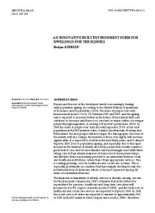
9 number of TAZs classified into each of the three categories (interpreted here as urban, suburban, and exurban). The naïve approach classified roughly 27% as urban, 43% as suburban, and 30% as exurban (Appendix 1). On the other hand, both cluster and PCA classified approximately 14% as urban, 37% as suburban, and 49% as exurban. The naïve approach groups more TAZs towards the middle of the distribution (suburban), and PCA and cluster analysis classify fewer TAZs as highly urban (Appendix 1). Accordingly, the PCA and cluster approaches had the highest agreement (92.9%) and the highest kappa statistic (0.88). A kappa statistic of 1 indicates perfect agreement and 0.8 is generally accepted as almost perfect agreement (24). Thus, the results suggest that the three methods have adequate levels of agreement. The naïve and cluster methods had 69.6% agreement and a kappa statistic of 0.54, while the naïve method and PCA 65.9% agreement and a kappa statistic of 0.48. All kappa statistics are significant at a 99% level of confidence. In summary, the analytical methods to calculate the BEI have high agreement, but PCA and cluster analysis agree the most. This suggests that implementation of the BEI does not require the use of all three approaches; instead they can rely on the approach that best fits the needs of the situation at hand. Comparisons with the PEF The PEF ranges from 4 to 12, with higher values indicating higher support for walking and bicycling. Therefore, we first treated the PEF as a continuous variable and compared it with the BEI scores for the PCA and the naïve approach (Table 3). The estimated Pearson correlation coefficient between the PEF and the PCA and the naïve method was 0.71 for both methods, indicating adequate agreement. Next the PEF was classified into three groups, as described in Section 3, in order to compare it to the cluster analysis. The PCA method had a slightly higher percent agreement with the PEF (67.2%) and a kappa statistic of 0.46, indicating moderate agreement. Both the cluster analysis method and the naïve method had lower agreement with the PEF (64.2% and 58.8%, respectively) and had slightly lower kappa statistics (0.42 and 0.38 respectively). Figure 3 depicts differences between the cluster analysis method and the PEF (left map) and the PCA method and the PEF (right map). TABLE 3 Comparison of three methods to calculate environmental indices with Portland’s PEF Pearson correlation Percent agreement with Weighted kappa with PEF PEF statistic with PEF (Raw BEI scores) (Three categories) (Three categories) PCA

0.71

67.2%

0.46

Naïve method

0.71

58.8%

0.38

Cluster analysis

N.A

64.2%

0.42

N.A. Not applicable. All Pearson correlation coefficients and kappa statistics are significant at a 99% level of confidence.

Taken together, these results suggest that the BEI and the PEF have a high degree of overlap, but they do not fully agree. Either the BEI and the PEF measure similar constructs differently, or they measure different constructs. Indeed, the indices vary not only in the numbers and types of

10 environmental attributes that compose them, the tools used (the BEI relies on a desktop approach while the PEF relies on a field survey), the way they are combined into a single score (objective rank/factor/cluster analysis versus objective Delphi- like process), but also in the outcome. While they share connectivity and accessibility concepts, they appear to measure these concepts in distinct ways. One option that limits the agreement between the measures is that the items constituting the PEF may correlate better with our third, pedestrian and bicycle domain, but not with our other two domains. To explore this, we separately correlated each of our domains to the PEF. We found that our third domain had the lowest correlation with the PEF of all three domains. 7 This result has two implications. First, it suggests that the BEI may be measuring a different, complementary construct than the PEF. Second, by showing that the BEI score correlates substantially better with the PEF than its individual components, the results underscore the synergy between the various items within the BEI.

Portland Study Area Built Environment Classification (by Traffic Analysis Zone)

Cluster Analysis and PEF Comparison

Cluster Analysis Minus PEF

Portland Study Area Built Environment Classification (by Traffic Analysis Zone)

PCA Minus PEF

-2

-2

-1

-1

0

0

1

1

2 Over-classification means the BEI classifies as area as more urban than the PEF. Under-classification means the BEI classifies an area as less urban han the PEF.

PCA and PEF Comparison

0

2.5

5

10 Miles

¯

2 Over-classification means the BEI classifies as area as more urban than the PEF. Under-classification means the BEI classifies an area as less urban han the PEF.

0

2.5

5

10 Miles

¯

Figure 3 Comparison of cluster and PCA methods with PEF 5. DISCUSSION AND CONCLUSIONS This study compared three methods of creating a composite index of the built environment using the Portland area as an example. It also compared the index calculated with these three methods to Portland’s well-researched PEF. The index proposed contains density measures, a simple representation of housing/ jobs balance and land use mix (housing, employment, and park density), and incorporates the concepts of accessibility, connectivity (sidewalk measures, roadway measures, and percent commuting by walk/ bicycle modes) and mobility (bus lines, light rail stations, percent commuting by transit). A comparison of the three methods revealed a strong degree of internal consistency between them, with principal components analysis appearing slightly superior to the naïve me thod and the cluster analysis method. Our comparison between the BEI and the PEF revealed considerable 7

Pearson coefficients for rank score averages for the domains are: development intensity, 0.66; motorized transportation, 0.65; and pedestrian and bicycle, 0.58. All va lues are significant at a 99% level of confidence.

11 consistency between the two and highlighted strengths and weaknesses of the BEI. The BEI proposed may be preferred to field survey approaches for at least three reasons. First, the BEI is readily accessible to many planning departments and its implementation is straightforward. Second, because the BEI utilizes secondary data and can be implemented relatively easily using GIS and basic statistical packages, it could result in considerable savings in staff time. Third, the BEI yields an objective analysis independent of the perspective of the researcher or planning staff. For indices based on primary data collected using Delphi methods, such as the PEF, there are concerns over the consistency and reliability of field survey scores assigned by different individuals, which also limits inter-regional comparisons. There are several ways in which the BEI could be improved. One limitation of relying heavily (although not entirely) on established census data is the absence of land use information. Therefore, the BEI cannot directly account for land use mixtures. Many studies have shown that this is a critical attribute that explains the behavior of travelers (25-28). Although the BEI does not contain a land use mix variable per se, it does include housing unit density and job density, which can act as surrogates for land use mixtures. Another area of improvement for the BEI is the low spatial resolution and on-the- ground verification that more disaggregate approaches might provide. TAZs are rather large and heterogeneous. Krizek (2003), for example, addressed this challenge for the purposes of measuring neighborhood accessibility by standardizing and reducing of the size of the units to a 150- meter grid. Such an approach, if applied to the BEI, could provide a more manageable scale of analysis. Modifying the index may allow for some gains in accuracy at the neighborhood level but the impact of modifications on the time and ease of implementation of the index should be understood. Increasing the time cost of acquiring data or the degree of sophistication of the GIS analysis may hamper the use of the BEI. While our goal was to complete the analysis with U.S. Population Census data only, we were unable to fully achieve this aim due to the limited types of data available and had to rely in part on additional sources. Sidewalk coverage data are not widely available in many communities. Although transit and park data are more common, these data are often not in a GIS format, limiting the implementation of the BEI. Finally, although our results may not be transferable to evaluate indices developed for other purposes, our methods and analytical approach are directly transferable. Further research should examine the ability to generalize from the current index to other study areas. Despite these limitations, the BEI provides a useful entry point for planners and researchers in examining the built environment. As more resources become available, the BEI can be tailored to particular needs in planning practice, applied research, or survey sampling. Focused research questions can guide modificatio ns to the index as well as an examination of its predictive validity. We suggest that the BEI should be utilized as an overview tool to identify built environments supportive of active transportation. 6. ACKNOWLEDGMENTS Preparation of this manuscript was supported by a grant from the Robert Wood Johnson Foundation Active Living Research program. We are grateful to Professor Yan Song for her assistance with GIS and for her guidance with the Portland data from the RLIS Lite CD. Many

12 thanks to Lisa Crook fo r her invaluable help solving numerous GIS challenges. Special thanks to Michael Greenwald, Ph.D. (University of Wisconsin) for the PEF shapefiles, Marc Schlossberg, Ph.D. (University of Oregon) for sidewalk files, and Mark Bosworth (Metro) for historic Portland data.

13

7. REFERENCES 1. Replogle, M., Integrating Pedestrian and Bicycle Factors into Regional Transportation Planning Models: Summary of the State-of-the Art and Suggested Steps Forward. Environmental Defense, Washington, D.C. 1995. 2. Krizek, K., Operationalizing Neighborhood Accessibility for Land Use-Travel Behavior Research and Regional Modeling, Journal of Planning Education and Research, vol. 22, 2003, pp. 270-287. 3. Frank, L., J. Sallis, B. Saelens, L. Leary, K. Cain, T. Conway, and P. Hess, A Walkability Index and Its Application to the Trans-Disciplinary Neighborhood Quality of Life Study, Journal of Planning Education and Research, Under review, 2004. 4. Cervero, R. and K. Kockelman, Travel Demand and the 3ds: Density, Diversity and Design, Transportation Research D, vol. 2, 1997, pp. 199-219. 5. Cervero, R. and M. Duncan, Walking, Bicycling, and Urban Landscapes: Evidence from the San Francisco Bay Area, American Journal of Public Health, vol. 93, 2003, pp. 14781483. 6. Ulmer, J. and L. Hoel, Evaluating the Accessibility of Residential Areas for Bicycling and Walking Using Gis. UVACTS-5-14-64. University of Virginia, Center for Transportation Studies 2003. 7. Srinivasan, S., Quantifying Spatial Characteristics of Cit ies, Urban Studies, vol. 39, 2002, pp. 2005 - 2028. 8. Ewing, R., T. Schmid, R. Killingsworth, A. Zlot, and S. Raudenbush, Relationship between Urban Sprawl and Physical Activity, Obesity, and Morbidity, American Journal of Health Promotion, vol. 18, 2003, pp. 47-57. 9. Jago, R., T. Baranowski, I. Zakeri, and M. Harris, Observed Environmental Features and the Physical Activity of Adolescent Males, American Journal of Preventive Medicine, vol. 29, 2005, pp. 98-104. 10. Clifton, K., A. Livi, and D. A. Rodriguez, Development and Testing of an Audit for the Pedestrian Environment, Under review, 2005. 11. Pikora, T., F. Bull, K. Jamrozik, M. Knuiman, B. Giles-Corti, and R. Donovan, Developing a Reliable Audit Instrument to Measure the Physical Environment for Physical Activity, American Journal of Preventative Medicine, vol. 23, 2002, pp. 187-194. 12. Moudon, A. V. and C. Lee, Walking and Biking: An Evaluation of Environmental Audit Instruments, American Journal of Health Promotion, vol. 18, 2003, pp. 21-37. 13. Blackman, A. and A. Krupnick, Location-Efficient Mortgages: Is the Rationale Sound?, Journal of Policy Analysis and Management, vol. 20, 2001, pp. 633. 14. Song, Y. and G. J. Knapp, Measuring Urban Form, Journal of the American Planning Association, vol. 70, 2004, pp. 210-226. 15. Caughy, M. O., P. J. O’Campo, and J. Patterson, A Brief Observational Measure for Urban Neighborhoods, Health & Place, vol. 7, 2001, pp. 223-236. 16. Streiner, D. L. and G. R. Norman, Health Measurement Scales : A Practical Guide to Their Development and Use, 3rd ed. Oxford ; New York: Oxford University Press, 2003. 17. Parsons Brinckerhoff Quade Douglas, The Pedestrian Environment. 1000 Friends of Oregon, Portland, Oregon 1993.

14 18. Cambridge Systematics, I., Short-Term Travel Model Improvements. DOT-T-95-05. Travel Model Improvement Program, U.S. Department of Transportation 1994. 19. Greenwald, M. J. and M. G. Boarnet, Built Environment as Determinant of Walking Behavior: Analyzing Nonwork Pedestrian Travel in Portland, Oregon, Transportation Research Record, vol. 1780, 2001, pp. 33-42. 20. Chicago Area Transportation Study, Conformity Analysis Documentation, Appendix A. Chicago, IL 2003. 21. Cervero, R., Built Environments and Mode Choice: Towards a Normative Framework, Transportation Research Part D, vol. 7, 2002, pp. 265-284. 22. Ewing, R. and R. Cervero, Travel and the Built Environment, Transportation Research Record, vol. 1780, 2001, pp. 87-114. 23. Jenks, G. F., The Data Model Concept in Statistical Mapping, International Yearbook of Cartography, vol. 7, 1967. 24. Landis, J. R. and G. G. Koch, The Measurements of Observer Agreement for Categorical Data, Biometrics, vol. 33, 1977, pp. 159-174. 25. Cervero, R., Mixed Land-Uses and Commuting: Evidence from the American Housing Survey, Transportation Research A, vol. 30, 1996, pp. 361-377. 26. Moudon, A. V., P. M. Hess, M. C. Snyder, and K. Stanilov, Effects of Site Design and Pedestrian Travel in Mixed-Use, Medium-Density Environments, Transportation Research Record, vol. 1578, 1997, pp. 48-55. 27. Frank, L. D. and P. O. Engelke, The Built Environment and Human Activity Patterns: Exploring the Impacts of Urban Form on Public Health, Journal of Planning Literature, vol. 16, 2001, pp. 202-218. 28. Khattak, A. and D. Rodriguez, Travel Behavior in Neo-Traditional Developments: A Case Study from the U.S.A, Transportation Research A, vol. 39, 2005, pp. 481-500.

15 APPENDIX 1 Comparison of TAZ classification into three BEI categories by method of computation Naïve method

Cluster method

PCA method

Urban

Suburban

Exurban

Urban

Suburban

Exurban

Urban

Suburban

Exurban

Number of TAZs Development intensity domain

236

370

267

126

338

409

121

312

440

Population density Housing unit density Employment density Park density

9.38 4.18 9.86 0.01

5.33 1.63 1.80 0.01

2.40 0.48 0.64 0.00

11.32 5.30 15.45 0.01

6.55 2.28 2.30 0.01

2.91 0.68 1.07 0.00

11.35 5.32 15.98 0.01

6.86 2.46 2.62 0.01

2.99 0.69 0.94 0.00

Motorized transportation domain Roadway density

0.04

0.02

0.01

0.05

0.03

0.02

0.05

0.03

0.02

0.03 12.6% 0.58

0.01 5.7% 0.00

0.00 3.4% 0.00

0.04 17.2% 0.93

0.02 6.4% 0.05

0.01 4.0% 0.00

0.04 17.3% 0.96

0.02 7.0% 0.06

0.01 3.8% 0.00

0.06 1.51

0.02 0.92

0.01 0.44

0.08 1.67

0.03 1.14

0.01 0.53

0.08 1.69

0.03 1.11

0.01 0.59

8.8%

3.2%

2.9%

11.4%

3.4%

3.5%

11.7%

4.0%

3.1%

Bus route density Transit commuting Proximity to subway station Pedestrian and bicycle domain Sidewalk density Sidewalk coverage Pedestrian and bicycle commuting