An Efficient Parallel All-Electron Four-Component Dirac−Kohn−Sham ...

384

J. Chem. Theory Comput. 2010, 6, 384–394

An Efficient Parallel All-Electron Four-Component Dirac-Kohn-Sham Program Using a Distributed Matrix Approach Loriano Storchi,† Leonardo Belpassi,† Francesco Tarantelli,*,† Antonio Sgamellotti,† and Harry M. Quiney‡ Dipartimento di Chimica and I.S.T.M.sC.N.R., UniVersita` di Perugia, 06123, Italy, and ARC Centre of Excellence for Coherent X-ray Science School of Physics, The UniVersity of Melbourne, Victoria, 3010, Australia Received October 12, 2009

Abstract: We show that all-electron relativistic four-component Dirac-Kohn-Sham (DKS) computations, using G-spinor basis sets and state-of-the-art density fitting algorithms, can be efficiently parallelized and applied to large molecular systems, including large clusters of heavy atoms. The performance of the parallel implementation of the DKS module of the program BERTHA is illustrated and analyzed by some test calculations on several gold clusters up to Au32, showing that calculations with more than 25 000 basis functions (i.e., DKS matrices on the order of 10 GB) are now feasible. As a first application of this novel implementation, we investigate the interaction of the atom Hg with the Au20 cluster.

I. Introduction Understanding the electronic structure and properties of molecules, clusters, and nanoscale materials containing heavy atoms represents a particularly challenging task for theory and computational science because the systems of interest have typically very many electrons, and both relativistic effects and electron correlation play a crucial role in their dynamics. The most rigorous way to introduce relativity in the modeling of molecular systems is to use the fourcomponent formalism derived from the Dirac equation. The method of choice is density functional theory (DFT) if many electrons are involved, as is the case with large metal clusters. In DFT, which is normally cast in the form of the independent-particle Kohn-Sham model, all of the exchangecorrelation effects are expressed implicitly as a functional of the electron density or, more generally, of the chargecurrent density.1,2 The relativistic four-component generalization of the Kohn-Sham method, usually referred to as the Dirac-Kohn-Sham (DKS) model, was introduced several years ago.3 Several modern implementations of this theory are available,4–7 including the one contained in our * Corresponding author e-mail: [email protected]. † Universita` di Perugia. ‡ The University of Melbourne.

own program, BERTHA.8–16 The full four-component DKS formalism is particularly appealing because it affords great physical clarity and represents the most rigorous way of treating explicitly and ab initio all interactions involving spin, which are today of great technological importance. The full four-component DKS calculations have an intrinsically greater computational cost than analogous nonrelativistic approaches or less rigorous quasi-relativistic approaches, mainly because of the four-component structure in the representation of the DKS equation, the complex matrix representation that usually arises as a consequence, the increased work involved in the evaluation of the electron density from the spinor amplitudes, and the intrinsically larger basis sets usually required. This greater computational cost, however, essentially involves only a larger prefactor in the scaling with respect to the number of particles or the basis set size, not a more unfavorable power law. Schemes have been devised in order to reduce the computational cost (see, e.g., refs 17–19 and references therein). A significant step forward in the effective implementation of the fourcomponent DKS theory is based on the electron-density fitting approach that is already widely used in the nonrelativistic context. Numerical density fitting approaches based on an atomic multipolar expansion7 and on a least-squares fit20 have in fact been employed in the four-component

10.1021/ct900539m  2010 American Chemical Society Published on Web 01/22/2010

A Four-Component Dirac-Kohn-Sham Program

relativistic domain. Recently, we have implemented the variational Coulomb fitting approach in our DKS method,14 with further enhancements resulting from the use of the Poisson equation in the evaluation of the integrals,15,21,22 and also from the extension of the density fitting approach to the computation of the exchange-correlation term.16 The above algorithmic advances have represented a leap forward of several orders of magnitude in the performance of the four-component DKS approach and have suddenly shifted the applicability bottleneck of the method toward the conventional matrix operations (DKS matrix diagonalization, basis transformations, etc.) and, especially, to the associated memory demands arising in large-system/large-basis calculations. One powerful approach to tackle these problems and push significantly further forward the applicability limit of all-electron four-component DKS is parallel computation with memory distribution. Analogous parallelization efforts of nonrelativistic DFT codes have already been described in the literature.23,34 The purpose of the present paper is to describe the successful implementation of a comprehensive parallelization strategy for the DKS module of our code BERTHA. In section II, we briefly review the DKS method as currently implemented in BERTHA and the computational steps making up a SCF iteration. In section III, we describe in detail the parallelization strategies adopted here. In section IV, we discuss the efficiency of the approach as results from some large all-electron test calculations performed on several gold clusters. Finally, we will present an actual chemical application of the method for the all-electron relativistic study of the electronic structure of Hg-Au20 with a large basis set.

II. Overview of the SCF Procedure In this section, we will briefly review the DKS method as it is currently implemented in BERTHA. We will mainly underline its peculiarities, especially in relation to the densityfitting procedure, and summarize the steps making up a SCF iteration and their typical serial computational cost for a large case. Complete details of the formalism can be found in refs 8, 9, 11, 14–16. In BERTHA, the large (L) and small (S) components of the spinor solutions of the DKS equation are expanded as linear combinations of Gaussian G-spinor basis functions. A peculiar and important feature of the BERTHA approach TT is that the density elements, ρµν (r), which are the scalar products of pairs of G spinors (labeled by µ and ν, with T ) L, S), are evaluated exactly as finite linear combinations of scalar auxiliary Hermite Gaussian-type functions (HGTF). This formulation9,11 enables the highly efficient analytic computation of all of the required multicenter G-spinor interaction integrals. In the current implementation of BERTHA, the computational burden of the construction of the Coulomb and exchange-correlation contributions to the DKS matrix has been greatly alleviated with the introduction14,15 of some effective density fitting algorithms based on the Coulomb metric, which use an auxiliary set of HGTF fitting functions. The method results in a symmetric, positive-definite, linear system,

J. Chem. Theory Comput., Vol. 6, No. 2, 2010 385

Ac ) v

(1)

to be solved in order to obtain the vector of fitting coefficients, c. The procedure involves only the calculation of two-center Coulomb repulsion integrals over the fitting basis set, Aij ) 〈fi||fj〉, and three-center integrals between the TT fitting functions and G-spinor density overlaps, ITT i, µν ) 〈fi||ρµν〉. The vector v in eq 1 is simply the projection of the electrostatic potential (due to the true density) on the fitting functions: Vi ) (fi ||ρ) )

TT TT Dµν ∑ ∑ Ii,µν

(2)

T)L,S µν

TT are the density matrix elements.14 In our where Dµν implementation, we take further advantage of a relativistic generalization of the J-matrix algorithm11,25,26 and an additional simplification arising from the use of sets of primitive HGTFs of common exponents and spanning all angular momenta from zero to the target value (for details, see ref 14). The auxiliary fitted density can be directly and efficiently used for the calculation of the exchange-correlation potential,27–29 and we have implemented this procedure in our DKS module.16 It is based on the solution a linear system similar to the Coulomb fitting one:

Az ) w

(3)

where the only additional quantity to be computed is the vector w representing the projection of the “fitted” exchangecorrelation potential onto the auxiliary functions: wi )

∫ Vxc[ρ˜(r)] fi(r) dr

(4)

The elements of the vector w, involving integrals over the exchange-correlation potential Vxc, are computed numerically by a standard cubature scheme.8 The cost of this step tends to become negligible, scaling linearly with both the number of auxiliary functions and the number of integration grid points. In the integration procedure, we again take advantage of our particular choice of auxiliary functions: the use of primitive HGTFs that are grouped together in sets sharing the same exponent minimizes the number of exponential evaluations at each grid point. Further computational simplification arises from using the recurrence relations for Hermite polynomials in the evaluation of the angular part of the fitting functions and their derivatives.28 Using the above combined approach, the Coulomb and exchangecorrelation contributions to the DKS matrix can be formed in a single step: TT TT + K˜µν ) J˜µν

TT (ci + zi) ∑ Ii,µν

(5)

i

We have found that the reduction of the computational cost afforded by the above density fitting scheme is dramatic. Besides reducing the scaling power of the method from O(N4) to O(N3), it reduces enormously the prefactor (by up to 2 orders of magnitude) without any appreciable accuracy loss.16 The application of the method to very large systems is, however, still impeded by the substatial memory require-

386

J. Chem. Theory Comput., Vol. 6, No. 2, 2010

Storchi et al.

tion necessary to obtain the density matrix from the occupied positive-energy spinors.

III. Parallelization Strategy

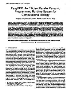
Figure 1. CPU time percentages for the various phases of a serial DKS calculation of the gold cluster Au16. All linear algebra operations are performed with the Intel Math Kernel Library.

ments imposed by huge basis sets and by the consequently large matrix dimensions. A truly practical parallelization scheme must inevitably tackle these aspects of the problem. Before we proceed to describe the parallelization of our code, it is useful to take a brief look at the time analysis of a typical serial SCF iteration of our DKS program, shown in Figure 1 for a realistically sized case: the Au16 cluster, with a DKS matrix dimension of 12 480. Here, we see that three O(N3) steps dominate the computation: diagonalization, J + K matrix computation, and the level-shifting phase. Thanks to the significant progress reviewed above, the J + K matrix computation time, formerly dominant, has been drastically reduced and, consequently, a larger time fraction (about half in the present example) is taken up by the diagonalization step. In our present serial implementation, the full DKS eigenvalue spectrum, comprising both the negative and positive energy halves, is computed. As we shall see later, we have adopted, in the parallel code, an effective reduction of the computed spectrum to the sole positiveenergy occupied spinors, which affords considerable time savings. Projection methods such as those proposed by Peng et al.,30 halving the size of the diagonalization problem, could also usefully be employed. We have not further investigated this point because, as hinted at above, our emphasis here is on the effective removal of the memory bottleneck for very large-scale applications, through data distribution. The J + K matrix computation, which takes about a third of the time, mainly involves the calculation of the three-index integrals Ii,TTµν and the implementation of eq 5. The remaining sixth of the time is used almost entirely in the level-shifting phase, which involves the double matrix multiplication transforming the DKS matrix from basis function space to spinor space. Clearly, the parallelization effort must target these three timeconsuming phases. It is remarkable that the entire densityfitting procedure, comprising the computation of the A, v, and w arrays and the solution of the associated linear systems of eqs 1 and 3, takes up an almost negligible fraction of the time. This phase, together with the HGTF expansion of the density, is bundled in the slice which we have labeled “Serial” in Figure 1, because we have left it unparallelized in the work described here. The remaining computation, labeled “Density”, involves essentially the matrix multiplica-

The code has been developed on a local HP Linux Cluster with an Intel Pentium D, 3.00 GHz CPU with a central memory of 4 GB on each node. The parallel implementation has been ported with success on a parallel SGI Altix 4700 (1.6 GHz Intel Itanium2 Montecito Dual Core) equipped with the SGI NUMAlink31 interconnect. All of the results in terms of scalability and speedup reported in the following have been obtained on the latter architecture. In the parallelization of the DKS module of BERTHA, we used the SGI implementation of the Message Passing Interface (MPI)32 and the ScaLAPACK library.33 The overall parallelization scheme we used can be classified as masterslave. In this approach, only the master process carries out the “Serial” portion of the SCF described in the previous section. All of the concurrent processes share the burden of the other calculation phases in Figure 1. We decided to use this approach because it is the easiest to code in order to make memory management especially convenient and favorable. Only the master process needs to allocate all of the large arrays, that is, the overlap, density, DKS, and eigenvector matrices. Each slave process allocates only some temporary small arrays when needed. In using this approach to tackle large molecular systems, it is crucial to be able to exploit the fast memory distribution scheme offered by the hardware. In particular, the SGI Altix 4700 is classified as a cc-NUMA (cache-coherent Non-uniform Memory Access) system. The SGI NUMAflex architecture34 creates a system that can “see” up to 128 TB of globally addressable memory, using the NUMAlink31 interconnect. The master process is thus able to allocate as much memory as it needs, regardless of the actual amount of central memory installed on each node, achieving good performances in terms of both latency and bandwidth of memory access. Some aspects of performance degradation related to nonlocal memory allocation will be pointed out later on. A. J + K Matrix Calculation. To parallelize the J + K matrix construction, the most elementary and efficient approach is based on the assignment of matrix blocks computation to the available processes. The optimal integral evaluation algorithm, exploiting HGTF recurrence relations on a single process, naturally induces a matrix block structure dictated by the grouping of G-spinor basis functions in sets characterized by common origin and angular momentum (see also ref 12). The master process broadcasts the c + z vector to the slaves at the outset of the computation. After this, an on-demand scheme is initiated. Each slave begins the computation of a different matrix block, while the master sets itself listening for messages. When a slave has finished computing one block, it returns it to the master and receives the sequence number identifying the next block to be computed. The master progressively fills the global DKS array with the blocks it receives from the slaves. A slave only needs to temporarily allocate the small blocks it computes.

A Four-Component Dirac-Kohn-Sham Program

This approach, as will be evident in the next sections, has several advantages. The communication time is essentially independent of the number of processes involved. The matrix blocks, although all relatively small, have different sizes, which tends to minimize communication conflicts, hiding communications behind computations. The small size of the blocks ensures optimal load balance and also permits a much more efficient use of the cache with respect to the serial implementation. B. Matrix Operations. The parallelization of the matrix operations which make up the bulk of the “level shift”, “diagonalization”, and “density” phases, has been performed using the ScaLAPACK library routines.33 There are two main characteristics of ScaLAPACK that we need to briefly recall here. First, the P processes of an abstract parallel computer are, in ScaLAPACK, mapped onto a Pr × Pc twodimensional grid, or process grid, of Pr process rows and Pc process columns (Pr · Pc ) P). The shape of the grid for a given total number of processors affects ScaLAPACK performance, and we shall briefly return to this point shortly. The second fundamental characteristic of ScaLAPACK is related to the way in which all of the arrays are distributed among the processes. The input matrices of each ScaLAPACK routine must be distributed, among all of the processes, following the so-called two-dimensional blockcyclic distribution.33 The same distribution is applied to the result arrays in output. For example, in the case of a matrix-matrix multiplication, the two input matrices must be distributed following the two-dimensional block cyclic distribution, and when the computation is done, the result matrix will be distributed among all of the processes following the same scheme. To simplify and generalize the distribution of arrays, and the collection of the results, we first of all implemented two routines using MPI, named DISTRIBUTE(mat,rank) and COLLECT(mat,rank). The first distributes the matrix mat, originally located on process rank, among all processes, according to the block cyclic scheme; the second carries out the inverse operation, gathering on process rank the whole matrix mat block-distributed among the available processes. It is worthwhile to note that both operations, as implemented, exhibit a running time that, for a given matrix size, is very weakly dependent on the number of processes involved. Except for a larger latency overhead, this time is in fact roughly the same as that required to transfer the whole matrix between two processes. Sample timings for the distribution and collection of four double-precision complex matrices of varying sizes are shown in Table 1. The four matrices are in fact the matrices occurring in the DKS calculations of the gold clusters described later in this work. The ScaLAPACK routines we used for the DKS program are PZHEMM in the “level shift” phase, PZGEMM in the “density” phase, and finally PZHEGVX to carry out the complex DKS matrix diagonalization. Before and after the execution of these routines, we placed calls to our DISTRIBUTE and COLLECT routines to handle the relevant matrices as required. The workflow is extremely simple. Initially, the DKS matrix is distributed to all processors. After this, the “level shift”, “diagonalization”, and “density” steps

J. Chem. Theory Comput., Vol. 6, No. 2, 2010 387 Table 1. Times in Seconds for the COLLECT (C) and DISTRIBUTE (D) Routines As a Function of Matrix Size and Number of Processors matrix dimension 1560

3120

6240

12480

number of processors

C

D

C

D

C

D

C

D

4 16 32 64 128

0.12 0.12 0.10 0.13 0.14

0.12 0.22 0.27 0.27 0.28

0.36 0.44 0.39 0.51 0.52

0.33 0.76 0.98 1.07 1.13

1.41 1.60 1.56 2.12 2.13

1.29 1.29 1.38 3.78 4.47

5.90 6.26 6.32 8.23 8.62

5.07 5.04 5.40 6.03 5.97

are performed in this order, exploiting the intrinsic parallelism of the ScaLAPACK routines. At the end, we collect on the master both the density matrix and the eigenvectors. Thus, apart from the internal communication activity of the ScaLAPACK routines, there are just four explicit communication steps, namely, the initial distribution of the DKS and overlap matrices and the final gathering of the resulting eigenvectors and density matrices. Note that the only communication time in the entire calculation that depends appreciably on the number of processors involved is that of the largely insignificant initial broadcast of the c + z vector, which is necessary to carry out the J + K matrix construction. Before we proceed, it is necessary to add a final note about the block cyclic decomposition. The scheme is driven, besides by the topology of the processes, by the size of the blocks into which the matrix is subdivided. This size is an important parameter for the overall performance of the ScaLAPACK routines. After some preliminary tests, we chose a block dimension equal to 32 (see also refs 24 and 35), and all of the results presented here are obtained using this block dimension. C. Notes about PZHEGVX Diagonalization. As we have seen at the end of section II, the DKS diagonalization phase takes up the largest fraction of computing time, and therefore all factors that affect its performance are important. While, for practical reasons, we could not investigate exhaustively all of these factors, we would like to highlight two of them which are particularly relevant in the present case. The PZHEGVX routine needs some extra work arrays to carry out the diagonalization. One can execute a special preliminary dummy call to PZHEGVX in order to obtain the routine’s estimate of the optimal size of this extra memory space for the case at hand. In our test applications, we noticed, however, that the estimated auxiliary memory was in fact insufficient to guarantee, especially for the larger systems, the full reorthogonalization of the eigenvectors (i.e., INFO > 0 and MOD(INFO/2,2) * 0). This appeared to cause some inaccuracies and instabilities in the final results. In order to avoid these problems and also to establish common comparable conditions for all of the test cases studied, we decided to require the accurate orthogonalization of the eigenvectors in all cases. This could readily be achieved by suitably enlarging the size of the work arrays until INFO ) 0. For example, in the case of the Au16 cluster (with a 2.4 GB DKS matrix), when 16 processors were used, the

388

J. Chem. Theory Comput., Vol. 6, No. 2, 2010

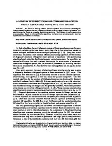
ScaLAPACK estimate of 180 MB per processor for the work arrays had to be raised to 400 MB to achieve complete reorthogonalization. Clearly, this strict requirement is quite costly in terms of both memory and computation time, and less tight constraints might be investigated and found to be acceptable in any given practical application. Another important aspect of ScaLAPACK diagonalization is that the PZHEGVX routine permits the selection of a subset of eigenvalues and eigenvectors to be computed. In the DKS computation, it is only essential, in order to represent the density and carry out the SCF iterations, to compute the “occupied” positive-energy spinors. This clearly introduces great savings in eigenvector computation, both in time and memory, because the size of such subset is a small fraction (about 10% in our tests) of the total. In principle, of course, selecting a subset of eigensolutions to be computed should not affect their accuracy. However, in order to ensure this numerically, so as to reproduce the results obtained by the serial code to working precision, we imposed the requirement that the computed positive-energy eigenvectors be strictly orthogonal to the ones left out. Orthogonality to the negative-energy part of the spectrum is guaranteed in practice by the very nature of the spinors and the very large energy gap that separates them. To ensure orthogonality between the occupied and virtual spinors, we found it sufficient to include a small number of lowest-lying virtuals in the computed spectrum, for which orthogonalization is explicitly carried out (as explained in the previous paragraph). We conservatively set this number of extra spinors at 10% of the number of occupied ones. As stated above, in all cases, the choice of parameters and conditions for the parallel calculations described here ensured exact reproduction of the serial results to double-precision accuracy. D. Notes on the ScaLAPACK Grid Shape. The shape of the processor grid arrangement presented to ScaLAPACK, for a given number of processors, may affect appreciably the performance of the routines. As suggested by the ScaLAPACK Users’ Manual,33 different routines are differently influenced in this regard. The performance dependence on the grid shape is, in turn, related to the characteristics of the physical interconnection network. While an exhaustive investigation of these aspects is outside the scope of the present work, we briefly explored the effect of the grid shape on the DKS steps of BERTHA which depend on ScaLAPACK. The results are summarized in Figure 2. This essentially reports, for some of the gold-cluster calculations discussed in depth in section IV, the relative performance of the diagonalization, level-shifting, and aggregate matrixoperation steps (including the small contribution of densitymatrix evaluation), observed with three different arrangements of a 16-processor array and, in the inset, a 64-processor array. In the 16-processor case, we looked at the square 4 × 4 grid shape and at the two rectangular shapes, 2 × 8 and 8 × 2, for the clusters Au2, Au4, Au8, and Au16. In the 64processor setup, we examined the 8 × 8, 2 × 32, and 32 × 2 arrangements in the case of Au16. The data obtained, as the figure indicates, do not allow us to draw definitive conclusions, but it is clear that the processor grid shape does indeed affect the performance of the various ScaLAPACK

Storchi et al.

Figure 2. Performance of DKS matrix operation steps with different ScaLAPACK processor grid shapes for a series of gold-cluster calculations discussed in the present work. Shown are the data for 16 processors (M ) 8) and for 64 processors (M ) 32, inset, for the sole Au16 cluster). The histogram bars labeled “Total” refer to the sum of all three matrix operation steps, including “Density”.

steps in different ways, also in dependence on the total number of processors. Lacking a general a priori model to predict the optimal grid shape in any given case and architecture, performing preliminary test calculations may be an important part of the optimization process. Both the data for P ) 16 and for P ) 64 seem to indicate that rectangular grids with Pr < Pc perform systematically better than the reverse arrangement for which Pr > Pc. The former is in fact also preferable over the square Pr ) Pc grid for the level-shifting phase. The data for P ) 16 suggest, however, that in the diagonalization step the square arrangement is to be preferred for small systems, while both rectangular shapes tend to become more efficient as the size of the problem increases. As a result, a Pr < Pc arrangement appears to be the globally optimal choice for large computational cases. The data for P ) 64 and Au16 in the inset, on the other hand, show that varying the number of processors may significantly alter the emerging pattern. In this case, for example, both rectangular grids appear again relatively unfavorable for the diagonalization step, so that the square arrangement is to be preferred overall. On the basis of the above results, we decided, for our further analysis, to use a square grid whenever possible and grids with Pr < Pc otherwise.

IV. Discussion We performed several computations for the gold clusters Au2, Au4, Au8, Au16, and Au32. To achieve fully comparable results throughout, we used neither integral screening techniques nor molecular symmetry in the calculations. The large component of the G-spinor basis set on each gold atom (22s19p12d8f) is derived by decontracting the double-ζquality Dyall basis set.36 The corresponding small component basis was generated using the restricted kinetic balance relation.11 The density functional used is the Becke 1988 exchange functional (B88)37 plus the Lee-Yang-Parr (LYP) correlation functional38 (BLYP). As auxiliary basis set, we use the HGTF basis called B20, optimized previously by us.14

A Four-Component Dirac-Kohn-Sham Program

J. Chem. Theory Comput., Vol. 6, No. 2, 2010 389

Table 2. CPU Times (s) for the Various Phases of DKS Calculations on Some Gold Clusters as a Function of the Number of Concurrent Processes Employed (Indicated by the ScaLAPACK Grid Shape) cluster

step

serial

2×2

4×4

4×8

8×8

8 × 16

Au2

J + K matrix diagonalization level shift density serial total iteration J + K matrix diagonalization level shift density serial total iteration J + K matrix diagonalization level shift density serial total iteration J + K matrix diagonalization level shift density serial total iteration J + K matrix diagonalization level shift density serial total iteration

24.75 33.32 10.20 0.57 5.19 74.03 183.50 262.07 83.87 4.48 22.01 555.93 1400.64 1976.78 679.52 35.64 106.36 4198.94 10946.55 17463.86 5598.50 293.90 580.43 34883.24

8.63 3.49 3.59 0.24 5.45 21.40 62.15 24.87 27.50 1.55 23.26 139.33 470.24 256.65 214.64 12.54 122.32 1076.39 3655.87 2639.84 2254.54 91.20 598.18 9239.63 28850.31 28851.37 17406.51 855.82 3632.59 79596.60

2.43 1.78 1.14 0.12 5.62 11.09 13.82 9.02 8.46 0.72 23.72 55.74 99.57 67.56 63.44 4.02 111.14 345.73 752.26 660.06 477.62 25.83 597.56 2513.33 5848.33 9950.42 5471.35 256.04 3684.21 25210.35

1.69 1.55 0.71 0.13 5.74 9.82 7.55 6.86 4.13 0.56 23.65 42.75 47.54 41.11 32.16 2.99 112.14 235.94 364.35 312.19 238.30 19.82 599.88 1534.54 2851.76 5100.27 2677.06 168.68 3729.45 14527.22

0.90 1.30 0.58 0.15 5.76 8.69 5.04 5.32 2.66 0.66 23.72 37.40 26.05 28.29 18.88 2.85 111.94 188.01 182.52 214.92 133.56 13.28 597.57 1141.85 1413.57 3197.00 1794.60 127.80 3692.64 10225.61

0.90 1.35 0.51 0.12 5.85 8.73 3.27 4.82 1.52 0.49 23.16 33.26 15.16 24.13 9.56 2.20 109.45 160.50 95.11 186.94 71.84 9.72 596.09 959.70 708.57 1926.66 695.77 73.31 3629.83 7034.14

Au4

Au8

Au16

Au32

A numerical integration grid has been employed with 61 200 grid points for each gold atom. The five Au clusters chosen offer testing ground for a wide range of memory requirements and double-precision complex array handling conditions: the DKS matrix sizes were 1560 for Au2 (37.1 MB), 3120 for Au4 (148.5 MB), 6240 for Au8 (594.1 MB), 12480 for Au16 (2.3 GB), and 24 960 for Au32 (9.3 GB). Table 2 reports some elapsed times of the phases of the SCF iterations, for the various gold clusters and different numbers of processors employed (shown in their Pr × Pc ScaLAPACK arrangement). Note that the parallel diagonalization times are disproportionately smaller than, and not comparable with, the serial times because the latter involve the computation of the whole spectrum of eigensolutions, while in the parallel cases we could adopt the selection described in section III.C. It should further be noted that the Au32 case was too demanding to be run on a single processor and that the times shown here are averages obtained from four SCF iterations. Figure 3 shows the corresponding speedup for the various cases. Because of the remarks just made concerning the serial diagonalization and the Au32 case, the speedup for the diagonalization step and for the entire Au32 calculation could not be computed with reference to the serial calculation. In these cases, the figure shows the relative speedup with respect to the four-processor case. This appears to be a consistent and reliable procedure. Note, for example, that the totaliteration serial time for Au32 estimated from the data of the 2 × 2 processor performance (2.79 × 105 s) agrees within 0.1% with the estimate one obtains by fitting an N3 power law to the serial times for the smaller clusters. In Figure 3,

we see that, with some exceptions, the speedup generally tends to increase with the size of the system under study. In particular, the time for the construction of the DKS matrix scales extremely well for large systems, reaching 91% and 95% of the theoretical maximum with 128 processors for Au16 and Au32, respectively. It should be noted that the maximum speedup is one less than the number of processors in the array because of the master-slave approach used here. The other phases of the calculation scale less satisfactorily, reflecting the performance limitations of the underlying ScaLAPACK implementation. This is especially evident for the calculation of the density matrix, which is however a particularly undemanding task and a small fraction (