search strategies, and (3) a decision variable selection heuristic more suitable .... important factor to be optimized. ...... Sequential SAT Engine for Circuits. Proc.
An Efficient Sequential SAT Solver With Improved Search Strategies F. Lu, M.K. Iyer, G. Parthasarathy, L.-C. Wang, and K.-T. Cheng Department of ECE, University of California at Santa Barbara Abstract A sequential SAT solver Satori [1] was recently proposed as an alternative to combinational SAT in verification applications. This paper describes the design of Seq-SAT – an efficient sequential SAT solver with improved search strategies over Satori. The major improvements include (1) a new and better heuristic for minimizing the set of assignments to state variables, (2) a new priority-based search strategy and a flexible sequential search framework which integrates different search strategies, and (3) a decision variable selection heuristic more suitable for solving the sequential problems. We present experimental results to demonstrate that our sequential SAT solver can achieve orders-of-magnitude speedup over Satori. We plan to release the source code of Seq-SAT along with this paper.
I. Introduction Boolean SAT finds applications in many areas of circuit design and verification such as Bounded Model Checking [2, 16], Unbounded Model Checking [13, 14], Redundancy Identification, Equivalence Checking [3], Preimage Calculation [15], etc. State-of-the-art SAT algorithms, as implemented in tools such as Z C HAFF [4], B ERKMIN [5], and C-SAT [6] have demonstrated that very hard SAT problems can now be solved in reasonable time. Bounded sequential search using SAT has been shown to be very effective in model checking. However, its major disadvantage is its lack of completeness in general sequential search. A sequential SAT solver Satori was proposed in [1], which utilizes combined ATPG and SAT techniques to realize a sequential SAT solver by retaining the efficiency of Boolean SAT and being complete in the search. Given a sequential circuit, we assume that the circuit follows the Huffman synchronous sequential circuit model as illustrated in Figure 1. Sequential SAT (or sequential justification) is the problem of finding an ordered sequence of input assignments to a sequential circuit, such that a desired objective is satisfied, or proving that no such sequence exists. A desired objective can be a collection of signal value constraints such as that a primary output is 1. In this paper, we focus on the sequential problems that initial states are given. PO
PO PI
PI Combinational
Combinational
Logic PPI
PO PI Combinational
Logic PPO
PPI
Logic PPO
PPI
PPO
Figure 1: Backward time-frame expansion
In sequential SAT, a sequential circuit is conceptually unfolded into multiple copies through backward time-frame expansion (Figure 1). In each time-frame, the circuit becomes combinational and hence, a combinational SAT solver can be applied. In each time-frame, a
K.C. Chen Design Technology Cadence Corporation
state element such as a flip-flop is translated into two corresponding signals: a pseudo primary input (PPI) and a pseudo primary output (PPO). The initial state is specified at the PPIs in time-frame 0. The objective is specified at the signals in time-frame n (the last timeframe, where n is unknown before solving the problem). While solving in an intermediate time-frames i (0 < i < n − 1), intermediate state solutions are produced at the PPIs and they become intermediate objectives for further justification in the previous time-frames i − 1. Seq-SAT has three major improvements over Satori:
State reduction As pointed out in the previous work [1], minimizing the set of assignments to the state variables, called state reduction, is a critical step for improving the efficiency of sequential search. Seq-SAT performs state reduction not only when an intermediate solution is produced but also when an intermediate state objective is proved unsatisfiable. In the first case, it employs an efficient two-step state reduction algorithm to obtain a smaller state clause. The algorithm follows a similar process as the D-algorithm [8] originally proposed for ATPG and utilizes 3-value simulation. For the second case, a different conflict analysis procedure rather than UIP based conflict analysis[12] is applied to derive a smaller state clause. Flexible sequential search framework Sequential search can be carried out in two strategies: depth-first or breadth-first. In the depth-first strategy, a SAT algorithm expands the search to a new timeframe whenever a solution state is identified for the current timeframe. If the backward justification fails in timeframe i − 1 and no state solution can be found, it then backtracks to timeframe i and select another state solution of timeframe i to continue the justification. In the breadth-first strategy, the state solutions in the current timeframe i are exhausted before expanding into a new timeframe i − 1. In this paper, we provide a flexible sequential search framework in which these two search strategies can be integrated. We introduce a priority-based search strategy that can combine both depthfirst search and breadth-first search and demonstrate its efficiency over other search strategies.
Decision variable selection heuristic In SAT, the idea that make decisions to satisfy recently deduced clauses[4, 5] has been proven to be very effective for solving hard combinational problems. However, when applying a combinational solver for sequential SAT, the run time of combinational SAT solving is not necessarily the most important factor to be optimized. In this paper, we propose a decision variable selection heuristic which is more suitable for solving sequential problems. The rest of the paper is organized as the following. Section II illustrates the use of combinational SAT in sequential SAT. In Section III, we discuss the importance of state reduction and describe our approaches to this problem. Section IV presents our sequential search framework. In Section V, we present our priority-based search strategy. Section VI discusses the impact of decision ordering in combinational SAT on the overall sequential SAT efficiency. Section VII summarizes experimental results to demonstrate the superiority of our current sequential SAT solver. Section VIII concludes the paper.
II. Combinational and sequential SAT Given a finite set of variables, V , over the set of Boolean values B ∈ {0, 1}, a literal, l/l is an instance of a variable or its complement, v/¬v ∈ V . A clause ci , is a disjunction of literals (l1 ∨ l2 . . . ∨ ln ). A formula f , is a conjunction of clauses c1 ∧ c2 . . . ∧ cn . A clause is considered as a set of literals, and a formula as a set of clauses. An assignment A satisfies a formula f if f (A) = 1. An assignment is called maximal when every variable in V receives a value assignment. Given a sequential circuit, a state clause is a clause consisting only of state variables. In a Boolean Satisfiability (SAT) problem (or here call it combinational SAT to differentiate from sequential SAT), a formula f is given and the problem is to find an assignment A to satisfy f or prove that no such an assignment exists. SAT has attracted tremendous research effort in recent years, resulting in the developments of various efficient SAT solver packages such as [4, 5, 6, 10, 11]. Through backward timeframe expansion (Figure 1), a sequential SAT problem can be translated into a sequence of combinational SAT problems.
II-A. Sequential SAT and state clauses
1. After solution state reduction, a solution is found whose state part contains the initial state. For example, a solution with the state part (x = 1, z = 1) contains the initial state (x = 1, y = 0, z = 1). In this case, a solution for the sequential SAT problem is found. Note that a solution without any assignments to PPIs contains any initial state.
Initial state: (x=1, y=0, z=1) (1)
time−frame n a b c
PPO x PPO y PPO z
PPI z No solution: UNSAT
1 a 0 b 0 c
f=1
PPI x PPI y
(3)
time−frame n
a b c
time−frame (n−1)
PPI x PPI y PPI z
state clause: (x+y’)
0 PPI 1 PPI
x
0 PPI
z
state objective
(2) f=1
PPO x PPO y PPO z
y
a b c
time−frame n f=1
PPO x PPO y PPO z
PPI x PPI y
PPO x 0 PPO y 1 PPO z
PPI z state clause: (x+y’)(x)
reaching state solutions contained by the state sub-space (x = 0, y = 1) in time-frame n − 1. The new combinational SAT instance is then passed to the Boolean SAT solver. Suppose in time-frame n − 1, no solution can be found for state objective (PPOx = 0, PPOy = 1). Then, we backtrack to time-frame n to find another solution. In a way, we have proved that from state (x = 0, y = 1), there exists no solution. Therefore, there is no need to remove the state clause (x + y0 ). However, at this point it is beneficial to perform further analysis to determine if both PPOx = 0 and PPOy = 1 are involved in the conflict that indicates state objective (PPOx = 0, PPOy = 1) is unsatisfiable. Suppose after conflict analysis, It is discovered that only PPOx = 0 is involved in the conflict. A state clause ”(x)” is then added. The future combinational SAT instances will then have the state clauses ”(x + y0 )(x)” included, that record the non-solution state sub-spaces previously identified. This is illustrated in (4) of the Figure. We call this step objective state reduction since it tries to derive a smaller state clause when a state objective becomes unsatisfiable. The solving continues until either one of the following two conditions is reached:
(4)
Figure 2: Sequential SAT with state clauses
To illustrate the usage of state clauses in sequential SAT, Figure 2 depicts a simple example circuit with three primary inputs a, b, c, one primary output f , and three state elements x, y, z. The initial state is (x = 1, y = 0, z = 1). Suppose the SAT objective is to satisfy f = 1. Starting from time-frame n where n is unknown, the circuit is translated into a combinational copy with state variables duplicated as PPOs and PPIs. This is illustrated as (1) in the Figure. Since this represents a combinational SAT problem, a Boolean SAT solver can be applied. Suppose after the combinational SAT solving, a solution (a = 1, b = 1, c = 0, PPIx = 0, PPIy = 1, PPIz = 0) for satisfying f = 1 (step (2))is identified. Notice that all inputs have values assigned in this solution, even though it might not be necessary to have all of them assigned in order to satisfy f = 1. This phenomenon is due to the use of a combinational SAT solver as mentioned earlier. The assignments at PPIs implies a solution state (x = 0, y = 1, z = 0) that doesn’t contain the initial state. Instead of justifying the state (x = 0, y = 1, z = 0) in time-frame n−1, we can examine it first to check whether we can change as many of the assignments to don’t-cares while still satisfying the objective f = 1. Suppose after analysis, we determine that z = 0 is unnecessary, it can be removed from the solution state (x = 0, y = 1, z = 0) and a solution state (x = 0, y = 1) is derived. We call this step solution state reduction since it tries to remove the unnecessary state variable assignments from a solution. The solution state (x = 0, y = 1) doesn’t contain the initial state either, so it still needs to be justified in timeframe n − 1. Backward time-frame expansion can be achieved by adding a state objective (PPOx = 0, PPOy = 1) to the combinational copy of the circuit. Also, a state clause (x + y0 ) is generated to prevent
2. If backtracked to time-frame n, the initial objective f = 1 cannot be satisfied under the constraints imposed by all the state clauses added, then the original problem is unsatisfiable. This is equivalent to say: if any objective (including the initial objective f = 1 and all intermediate objectives) cannot be satisfied under the constraints imposed by all the state clauses added, then the original problem is unsatisfiable. The above example illustrates several important concepts in the design of our current sequential SAT solver. • The state reduction involves finding smaller state clauses in order to more effectively prune the search space. There are two types of state reduction. One is solution state reduction, the other is objective state reduction. • The use of state clauses serves two purposes: (1) to record those state sub-spaces that have been explored, and (2) to record those state sub-spaces containing no solution. The first is to prevent the search from entering a state justification loop. • Although conceptually the search follows the backward timeframe expansion, the above example demonstrates that in the implementation, explicit time-frame expansion is not necessary. In other words, a sequential SAT solver needs only one copy of the circuit. Moreover, there is no need to memorize the number of time-frames being expanded. Later we will discuss our implementation of the solver and demonstrate how this can be achieved by using an objective list. • The above example demonstrates the use of depth-first search strategy. However, by using state clauses, more flexible search strategies are feasible if the intermediate state objectives are recorded in a list. The idea of the sequential search framework can be described as follows: Given a sequential problem with an objective obj and an initial state s0 , C is the one time-frame combinational copy of the sequential circuit where each state variable is expanded to a PPI variable and a PPO variable. Suppose we use an objective list FO to store the intermediate objectives, and initially it only contains obj. Each time, an objective o is selected from FO and given to the combinational circuit solver.
The circuit solver then solves o on C. There will be three possible outcomes reported by the solver: (1) o is unsatisfiable, (2) at least one state in the obtained solutions contains the initial state s0 , and (3) no state in the obtained solutions contains the initial state s0 . For case (1), we can remove o from FO. For case (2), the search stops and the sequential problem is proven satisfiable. For case (3), the state part of each solution is added to FO as a new state objective and a state clause is added to C to prevent the state be explored and found again in any future solutions. If finally, the objective list FO becomes empty, which means all objectives have been proven to be unsatisfiable, then the search stops and the sequential problem is proven unsatisfiable. In this framework, the keys are to decide how to select the next objective from the list for solving and to decide how many solutions to be found for an objective each time. The details will be given in Section IV. In the following, we will describe the detail of Seq-SAT. To facilitate the description, we define the following two terms: (1) a frame objective is an objective to be satisfied which is passed to the combinational SAT solver. A frame objective can be either the initial objective or a state objective. (2) a frame solution is an assignment at the PIs and PPIs, which satisfies a given frame objective.
III. State reduction for state space pruning There are two types of state reduction: solution state reduction (SSR) and objective state reduction (OSR). SSR is performed when a frame solution is identified by the combinational SAT solver. OSR is applied when a state objective becomes unsatisfiable. The details are discussed in the following.
III-A. Solution state reduction When a frame solution is identified by the combinational SAT solver, all PIs and PPIs have assigned values. Our goal is to find and un-assign the unnecessary assignments at the PPIs. With fewer assigned PPIs, a smaller state clause can be created, which prunes a larger state sub-space. Given an initial frame solution, to derive one containing a minimal number of state variables with value assignment is an NP-complete problem. Therefore, we only derive a locally minimized 3-value solution. A frame solution s of a frame objective o is a locally minimized 3-value solution if and only if un-assign any state variable of s (changing its value from a 0/1 to X), the resulting assignments cannot satisfy o by 3-value simulation. One straight forward heuristic to derive a locally minimized 3value solution is to employ 3-value simulation. That is, for all assigned state variables of a solution, un-assign one of them at a time to check if its assignment is necessary to satisfy the frame objective. If not, the assignment is removed from the solution, this procedure continues until each assigned state variable has been checked once, then the remaining assignments form a 3-value minimized solution. A frame solution reported by a SAT solver usually contains many unnecessary assignments at state variables. Directly apply 3-value simulation could be computationally expensive. For example, removing N unnecessary state assignments needs at least N times of simulation even if parallel simulation is used. To reduce the number of simulation runs and improve efficiency, we adopt a two-step state reduction approach. In this approach, a modified D-algorithm [8] is first applied to obtain a minimized solution. Given a frame objective O and its frame solution S, the modified D-algorithm justify O based on S, that is, when the D-algorithm makes a decision at a signal, the value assigned to the signal has to be consistent with its value in the solution S. Hence, the D-algorithm is used as a trace procedure, not as a search procedure. Based on the minimized solution from the first step,
3-value simulation is then employed to derive a 3-value minimized solution. This approach is based on the assumption that the D-algorithm can usually find a solution containing much fewer assignments than that of a SAT solver. Experiments show our assumption is valid in general. The details of the approach are omitted due to page limit. TABLE I: R ESULTS OF SOLUTION STATE REDUCTION Circuit
Org #
Step 1 resulting Step 2 resulting # %reduced times(sec) # %reduced times(sec) s526 91134 70981 22.1% 1 70545 0.6% 1 s1423 237344 73986 69.1% 3 73298 0.4% 1 s5378 181487 89499 50.6% 9 87450 2.3% 2 s35932 3382 3142 7.1% 2 3142 0% 3 s38417 2008744 1054999 47.4% 280 1052562 0.2% 100 s38584 869942 375770 56.8% 128 371707 1.1% 110
Table I shows experimental results to demonstrate the impact of solution state reduction. All our experiments were run on P4 2GHz Linux machines with 1 GB memory. In these experiments, a sequence of sequential SAT problem instances are created for each circuit. For each circuit and each of its primary outputs f , the first SAT objective is to satisfy f = 1 and then we would try to satisfy f = 0. This is a typical primary output toggle experiment. The results shown for each circuit are for solving all toggle SAT instances for the circuit. We assume the initial state is that all state elements have a 0 value. Note, this kind of problems may contain very difficult cases even for ISCAS 89 circuits. The two ”#” columns show the numbers after state reduction with modified D-algorithm (step 1) and then, with three value simulation (step 2), respectively. The two ”% reduced” columns show the corresponding percentage of reduction. The two run-time columns show the run times based on using step 1 and then, using step 2. We note that if no state reduction is performed, then the sequential SAT might not finish solving all instances within a reasonable time for each of these examples. From the results, we can see that the modified D-algorithm could reduce most of the unnecessary assignments to the state variables, so the number of 3-value simulation runs can be greatly reduced. Although step 2 does not help much in terms of the total percentage of assignment reduction, it does help further improve the overall performance.
III-B. Objective state reduction As a state so is added to the objective list, a state clause sc is added to prevent the state from being reached again. When the state objective so becomes unsatisfiable, instead of using the same state clause sc, a smaller state clause might be added to prune a larger search space. This can be achieved by additional conflict analysis when a state objective is proved unsatisfiable. We explain the idea by an example, suppose the state objective so is (PPOr = 1, PPOs = 1, PPOt = 0, PPOx = 0, PPOy = 1), the implication graph when sc is proved unsatisfiable (which means there is a conflict that can not be resolved by backtrack) is shown as in Figure 3. From Figure 3, if tracing from the conflict points to the PPO state variables, we can deduce that (PPOr = 1, PPOs = 1, PPOt = 0) is unsatisfiable, so the state clause (r 0 + s0 + t), which is smaller than (r 0 + s0 + t + x + y0 ), can be added to the circuit. However, we need to be careful that the state clauses added in this way shouldn’t exclude the search space that contains the initial state. Otherwise a satisfiable problem erroneously becomes unsatisfiable since the initial state couldn’t be reached anymore after adding such a state clause. Using the above example, if the values of r, s and t in the initial state are 1, 1 and 0 respectively, state clause (r 0 + s0 + t) would exclude the initial state. To avoid this, we can just select a state variable from the state objective whose objective value is not its initial value and add its corresponding literal to the state clause. For example, if the value of x in the initial state is
1 in the above example, we can add x0 to the state clause (r 0 + s0 + t) to form state clause (r 0 + s0 + t + x0 ) which can be added to the circuit. This can always be done since state objectives don’t contain the initial state. That is, each state objective must have at least one variable whose objective value is not same as its value in the initial state, otherwise, the problem should has been proved satisfiable. This reduction is valid even if state clauses that were used for preventing justification loop are involved in the conflict graph. We also note that this reduction is not related to identify the subset of a CNF formula that is sufficient for unsatisfiability, instead, it just tries to find a conflict clause that contains only literals of the variables in a state objective. Table II gives the experimental results comparing the performance of our sequential solver with and without OSR. These are the same toggle experiments as those in Table I. TABLE II: E FFECTS OF O BJECTIVE S TATE R EDUCTION Without OSR With OSR Circuit runtimes(sec) stats runtimes(sec) stats s526 2 12/0/0 1 12/0/0 s1423 1 10/0/0 1 10/0/0 s5378 402 89/5/4 3 90/8/0 s13207 1924 165/58/19 1345 166/63/13 s15850 2002 100/54/20 522 100/69/5 s35932 3 640/0/0 3 640/0/0 s38417 286 210/0/2 100 212/0/0 s38584 106 498/58/0 111 498/58/0 **abort time for each problem is 100 sec. stats: x/y/z are #SAT/#UNSAT/#Abort
From the experiment results, it can be seen that the performance is greatly improved for half of the testcases by OSR, and only for one testcase, it causes a small overhead.
search, it demands the solver to find all solutions for the selected objective. After that, the objective is removed from the objective list. This framework further enables us to explore various search strategies between these two extreme ones which will be described later in this section. The overall framework of our sequential SAT solver is described in Algorithm IV.1. In the description, we assume that each frame objective produces at most one frame solution at a time. This assumption is only for purpose of easier explanation. The algorithm can be easily modified to serve the case that multiple solutions are produced at a time. The procedure PPO state conflict analysis() does objective state reduction, and state reduction() does solution state reduction. The procedure select a frame objective() selects a frame objective to be solved next, upon different implementation, various search strategies can be realized, and the details will be given in the next section. A frame objective can be removed from the objective list only if it is proven unsatisfiable by the combinational SAT. If it is satisfiable, the frame objective stays in the objective list. If the objective list becomes empty during the sequential search, it means that the solver has exhausted all the state objectives and, therefore, proved that the initial objective is unsatisfiable. Note that during each step of combinational SAT, conflict clauses are also accumulated through the combinational SAT solving process. When the sequential solving switches from one frame objective to another, these conflict clauses stay. Hence, in the sequential solving process, the conflict clauses generated by the combinational SAT are also accumulated. Our experience indicates that although these conflict clauses does help speed up the combinational SAT solving, for sequential SAT, the state clauses are the dominating source for the efficiency improvement of the overall sequential search. Algorithm IV.1: S EQUENTIAL S OLVER(C, ob j, s0 )
PPO
PPO
comment: C is the circuit with PPIs and PPOs expanded comment: ob j is the initial objective comment: s0 is the initial state
r
−f
s
e −PPO
t
comment: FO is the objective list Conflicting Variable
−c −d f
−PPO
PPO
y
x
b
−a
Figure 3: An implication graph when a state objective is proved unsatisfiable
IV. Flexible sequential search framework In our sequential SAT design, state clauses are accumulated through the solving process. The sequential solving process consists of a sequence of combinational solving tasks based on a given frame objective. At the beginning, the frame objective is the initial objective. As the solving proceeds, many frame solutions become frame objectives. These frame objectives are stored in the objective list. The use of state clauses and the objective list offer much flexibility in the choice of the search strategy. Different search strategies can be implemented by using different criteria in selecting the next frame objective for solving, and in deciding how many solutions to be obtained at a time for a frame objective. For example, for the depth-first search, the objective list is used as a stack where the next selected objective is the one most recently produced. For the breadth-first search, the objective list is used as a queue. In addition, in the breadth-first
FO ← {ob j}; / while(FO 6= 0) f ob j ← select a frame objective(FO); f sol ← combinational solve a frame objective(C, f ob j ); if ( f sol = NULL) clause ← PPO state conflict analysis(C, f ob j ); add state clause(C, clause); FO ← FO − { f }; ob j do state cube ← state reduction(C, f ob j , f sol ); if (s0 ∈ state cube) �return (SAT ); else clause ← convert to clause(state cube); else add state clause(C, clause); FO ← FO + {state cube};
return (UNSAT )
V. On the scheduling of frame objectives In this section, we introduce a new search strategy, called the priority-based search strategy, which can be easily implemented in the search framework described above. We further compare it with the depth-first and breadth-first search strategies and demonstrate its superiority. Given a state objective, we define its size as the total number of state variables minus the number of state variables with an binary objective value (i.e. not an unknown X) in the state objective. We use size(ob j) to denote the size of ob j. Note that a state objective with a larger size corresponds a larger state sub-space. Hence, if there are multiple state objectives in the objective list, it seems intuitive
to choose the largest state objective as the next objective for solving as it corresponds to exploring the solution with the largest state sub-space, and its solutions, if any, tend to contain fewer state assignments, which means smaller state clauses are likely to be generated to prune a larger search space. We further define the count of an objective ob j as the number of times that ob j has been selected for solving by the combinational solver. If we use count to guide the selection of objectives and choose the one with the largest count as the next objective, it will be more like the breadth-first search strategy. On the other hands, if we choose the one with the smallest count, It will be more like the depth-first search. Now we define priority of a frame objective ob j, pri(ob j), as follows:
Decision heuristic 2: First, the decision variable is selected from the most recently generated conflict clause that is not yet satisfied [5]. If all the generated conflict clauses are satisfied, the decision variable is selected based on the J-nodes [17, 6] with the highest topological order (closest to the POs and the PPOs). This decision heuristic is used in the original combinational SAT solver C-SAT [6]. Decision heuristic 3: First, the decision variable is selected from the most recently generated conflict clause that is not yet satisfied as in Heuristic 2 above. If all the generated conflict clauses are satisfied, the decision variable is selected from PIs and PPIs where PIs are selected before PPIs This is the default heuristic used in our final implementation.
pri(ob j) = size(ob j) − count(ob j)/10 (1) In our implementation of the priority-based search strategy, we select the objective with the largest value of pri. If there is a tie under this selection criterion, then the most recently generated one will be selected. For each selected objective, at most one solution is obtained at a time. Through extensive experiments, we observe that combining size and count in this way maximizing the performance, in general, for both satisfiable and unsatisfiable cases. With the objective list, depth-first and breadth-first search strategies can be implemented easily. In depth-first search, the list behaves like a stack. Hence, the selected objective is the one most recently produced. In breadth-first search, the list behaves like a queue. However, in breadth-first search, solving an objective means to finish producing all possible solutions. Then, the objective is removed from the objective list. Table III gives the experimental results comparing different search strategies. These are the same toggle experiments as those in Table I. The ”priority” column is the same as the last ”times” column in Table I. As it can be seen, the new search strategy significantly outperforms the depth-first and the breadth-first strategies.
The reasons we adopt Heuristic 3 in Seq-SAT are summarized as follows:
TABLE III: CPU RUNTIMES ( IN SECONDS ) ON
SEARCH STRATEGIES
depth-first breadth-first priority Circuit runtimes stats runtimes stats runtimes stats (sec) (sec) (sec) s526 9 12/0/0 2 12/0/0 1 12/0/0 s1423 301 7/0/3 103 9/0/1 1 10/0/0 s5378 1504 75/8/15 511 89/5/4 3 90/8/0 s13207 2159 167/54/21 1367 166/63/13 1345 166/63/13 s15850 1401 100/60/14 1569 100/59/15 522 100/69/5 s35932 32020 320/0/320 3 640/0/0 3 640/0/0 s38417 2324 189/0/23 2031 192/0/20 100 212/0/0 s38584 8515 414/57/85 2006 482/57/17 111 498/58/0 **abort time for each problem is 100 sec. stats: x/y/z are #SAT/#UNSAT/#Abort
VI. On the decision variable selection heuristics in the combinational SAT solver For pure combinational SAT, both VISDS[4] decision variable selection and clause based decision variable selection [5] have been proven effective. However, when applying a combinational SAT solver for sequential SAT, the runtime of combinational SAT solving is not the only critical factor. In each run of combinational SAT solving during the sequential SAT, the smaller the necessary assignments are made at the PPIs, the more efficiently the state space can be pruned. Therefore, the decision variable selection heuristics in combinational SAT also need modifications. To demonstrate this point, we conducted experiments to compare different decision variable selection heuristics in combinational SAT. Decision heuristic 1: This is the same as the VISDS decision variable selection [4].
(1). Using input variables as decision points results in better performance for easy combinational problems in general. For a sequential problem that can be transformed into a series of relatively easy combinational problems, this heuristic works very well. (2). For hard problems, as the conflict clauses tend to accumulate fast during search, the decisions will gradually be dominated by the conflict clauses. Therefore, the performance will not degrade much. (3). Selecting PIs prior to PPIs as decision variables tends to result in solutions with fewer state variables with value assignments [14]. TABLE IV: CPU RUNTIMES ON
DIFFERENT DECISION HEURISTICS
heuristic 1 heuristic 2 heuristic 3 Circuit runtimes stats runtimes stats runtimes stats (sec) (sec) (sec) s526 1 12/0/0 3 12/0/0 1 12/0/0 s1423 205 8/0/2 1 10/0/0 1 10/0/0 s5378 313 90/7/1 109 90/7/1 3 90/8/0 s13207 1436 166/62/14 1374 166/63/13 1345 166/63/13 s15850 511 100/69/5 514 100/69/5 522 100/69/5 s35932 3 640/0/0 3 640/0/0 3 640/0/0 s38417 194 211/0/1 253 210/0/2 100 212/0/0 s38584 41 498/58/0 300 496/58/2 111 498/58/0 c3540 40 0/1/0 13 0/1/0 20 0/1/0 c5315 21 0/1/0 16 0/1/0 8 0/1/0 **abort time for each problem is 100 sec. stats: x/y/z are #SAT/#UNSAT/#Abort
Table IV shows the results of different heuristics. The experiments for ”s-” circuits were the same PO toggle experiments circuit as explained before. The experiments for ”c-” circuits were the combinational equivalence checking problem using the miter circuit of two identical ISCAS 85 circuits. It can be seen that the decision heuristic 3 works well for sequential circuits, even for large combinational circuits, its performance is not bad.
VII. Additional experimental results Table V compares our solver with NuSMV [16] bounded model checking function for satisfiable cases. We have shown in the previous experiments how each idea works, Table VI compares the overall performance of Seq-SAT with Satori. In Table V, the ”Property” column gives the LTL formula for each testcase, and ”length” columns give the length of the witness vectors obtained by Seq-SAT and NuSMV respectively. For NuSMV, the version we used is NuSMV 2.1.2-zchaff in which the SAT solver zchaff is used for bounded model checking. The initial states used in these examples are all 0.
TABLE V: C OMPARISON TO N U SMV BOUNDED MODEL CHECKING Seq-SAT NuSMV Circuit Property runtimes(sec) length runtimes(sec) length s526 G(g214 = 0) 1 133 15 33 s13207 G(g594 = 0) 1 5 2 5 s13207 G(g785 = 0) 7 11 34 10 s38417 G(g5549 = 0) 9 815 > 3600 s38417 G(g16399 = 0) 14 7 55 7 s38584 G(g11678 = 0) 6 30 831 12 s38584 G(g29212 = 0) 48 144 > 3600 **abort time for each problem is 3600s.
From Table V, it can be seen that, even though the witness vectors derived by Seq-SAT are in general longer than those by NuSMV, SeqSAT clearly outperforms NuSMV in terms of CPU runtime. In Satori, the depth-first search and the breadth-first search are implemented separately. So in Table VI, we compare Seq-SAT with Satori under these two search strategies for the same toggle experiments as those in Table I. Table VII summarizes the number of the abort cases shown in Table VI. Column ”#Satori abort” shows the number of cases aborted in both Satori depth-first search and Satori breadth-first search. Column ”#SSANA” gives the number of cases aborted in Seq-SAT but not aborted in either Satori depth-first search or Satori breadth-first search. TABLE VI: C OMPARISON TO S ATORI Satori depth-first Satori breadth-first Seq-SAT Circuit runtimes stats runtimes stats runtimes stats (sec) (sec) (sec) s526 405 8/0/4 5 12/0/0 1 12/0/0 s1423 400 6/0/4 106 9/0/1 1 10/0/0 s5378 4100 53/4/41 1455 80/4/14 3 90/8/0 s13207 4010 154/48/40 1836 166/59/17 1345 166/63/13 s15850 2302 99/52/23 2214 100/52/22 522 100/69/5 s35932 3200 608/0/32 1 640/0/0 3 640/0/0 s38417 805 204/0/8 2257 191/0/21 100 212/0/0 s38584 4810 451/57/48 2228 477/58/21 111 498/58/0 **abort time for each problem is 100 sec. stats: x/y/z are #SAT/#UNSAT/#Abort TABLE VII: A BORTED C ASES A NALYSIS Circuit #Satori abort #Seq-SAT abort #SSANA s526 0 0 0 s1423 1 0 0 s5378 14 0 0 s13207 17 13 0 s15850 22 5 0 s35932 0 0 0 s38417 5 0 0 s38584 11 0 0
It can be seen that Seq-SAT achieves significant performance improvement for almost all cases. It is also interesting to note that the results of the depth-first search in Satori are quite different from those of depth-first search implemented in Seq-SAT (see Section V Table III). This indicates that the depth-first search is quite unstable (especially for satisfiable cases) and easy falls into bad search area.
VIII. Conclusion In this paper, we present an efficient sequential SAT solver SeqSAT. The implementation of Seq-SAT employs four new ideas: (1) better state reduction algorithms, (2) a more flexible search framework for accommodating and integrating different search strategies, (3) the priority-based search strategy, and (4) a modified decision variable selection heuristic for the underlying combinational circuit SAT solver. With these new ideas and efficient data structures and implementation, Seq-SAT achieves very significant speedup over Satori.
We will release the source code of Seq-SAT along with the publication of this paper.
References [1] M. K. Iyer, G Parthasarathy, K.-T. Cheng, SATORI - A Fast Sequential SAT Engine for Circuits. Proc. IEEE/ACM International Conference on Computer-Aided Design 2003. [2] A. Biere, A. Cimatti, E. M. Clarke, M. Fujita, and Y. Zhu, Symbolic Model Checking using SAT Procedures instead of BDDs. In Proc. of the 36th ACM/IEEE Design Automation Conf., pp. 317-320, June 1999. [3] P. Tafertshofer, A. Ganz, and K. Antreich, IGRAINE – An Implication-Graph based Engine for Fast Implication, Justification and Propagation. IEEE Trans. on Computer-Aided Design, 19(8):907–927, August 2000. [4] M. Moskewicz, C. Madigan, Y. Zhao, L. Zhang, and S. Malik, Chaff: Engineering an efficient SAT solver. Proc. of ACM/IEEE Design Automation Conf., pp. 530-535, June 2001. [5] E. Goldberg and Y. Novikov, BerkMin: A fast and robust Sat Solver. Proc. European Design and Test Conf., pp. 142-149, March 2002. [6] Feng Lu, Li-C. Wang, Kwang-Ting Cheng, A circuit SAT solver with signal correlation guided learning. In Proc. European Design and Test Conference 2003. [7] P. Tafertshofer, A. Ganz, and M. Henftling, A SAT-Based Implication Engine for Efficient ATPG, Equivalence Checking, and Optimization of Netlists. Proc. IEEE/ACM International Conference on Computer-Aided Design, pp. 648-655, Nov. 1997. [8] M. Abramovici, M. A. Breuer, and A. D. Friedman. Digital Systems Testing and Testable Design. CS Press, 1st ed., 1990. [9] G Parthasarathy, M. K. Iyer, Li-C. Wang and K.-T. Cheng, Efficient Reachability Checking and Pre-image Computation using Sequential SAT. Proc. Asia and South Pacific Design Automation Conf. 2004. [10] H. Zhang. SATO: An Efficient Propositional Prover. Proc. of International Conference on Automated Deduction, Vol 1249, LNAI, pp. 272-275, 1997 [11] J. P. Marques-Silva and K. A. Sakallah. GRASP: A Search Algorithm for Propositional Satisfiability. IEEE Trans on Computers, vol.48, pp. 506-521, 1999. [12] L. Zhang, C. Madigan, M. Moskewicz, and S. Malik. Efficient conflict driven learning in a Boolean satisfiability solver. Proc. IEEE/ACM International Conference on Computer-Aided Design, pp. 279-285, Nov. 2001. [13] K. L. McMillan. Applying SAT methods in unbounded symbolic model checking. Proc. of International Conference on Computer Aided Verification, Vol 2404, LNSC, pp. 250-264, 2002. [14] H.-J. Kang, I.-C. Park. SAT-Based Unbounded Symbolic Model Checking. Proc. of ACM/IEEE Design Automation Conf., pp. 840-843, June 2003. [15] B. Li, M. S. Hsiao, and S. Sheng. A novel SAT all-solutions solver for efficient preimage computation. Proc. of Design, Automation and Test in Europe Conf., pp. 10272-10277, Feb. 2004. [16] A. Cimatti, E. Clarke, E. Giunchiglia, et. al.. NuSMV 2: An OpenSource Tool for Symbolic Model Checking. In Proc. CAV’02, LNCS. Springer Verlag, 2002. [17] M.K.Ganai, L.Zhang, P.Ashar, A.Gupta, and S.Malik. Combining strengths of circuit-based and CNF-based algorithms for a high-performance SAT solver. In Proc. ACM/IEEE Design Automation Conf., pp. 747-750, June 2002.