U NIVERSITEIT VAN
A MSTERDAM IAS technical report IAS-UVA-05-03
An Efficient Spatially Constrained EM Algorithm for Image Segmentation Aristeidis Diplaros1 , Theo Gevers1 , and Nikos Vlassis2 1
Intelligent Sensory Information Systems, University of Amsterdam , The Netherlands 2 Intelligent Autonomous Systems, University of Amsterdam , The Netherlands
We present a novel EM algorithm for model-based image segmentation which incorporates efficient and economical spatial constrains among pixels via a Markov random field model. We adopt a generative model in which the unobserved class labels of neighboring pixels in the image are assumed to be generated by prior distributions with similar parameters. We derive a penalized log-likelihood optimization procedure for estimating the parameters of the pixels’ labels priors, and those of a Gaussian observation model that is shared among pixels. Our algorithm is very easy to implement and is similar to the standard EM algorithm for Gaussian mixtures, with the main difference that the labels posteriors are ‘smoothed’ over pixels between each E- and M-step by a standard image filter. Experiments on synthetic and real images show that our algorithm achieves competitive segmentation results compared to other Markov-based methods, and is in general faster. Keywords: Image segmentation, Hidden Markov random fields, EM algorithm, Bound optimization, Spatial clustering.
IAS
intelligent autonomous systems
An Efficient Spatially Constrained EM Algorithm for Image Segmentation
Contents
Contents 1 Introduction
1
2 Models 2.1 Standard mixture model . . . . . . . . . . . . . . . . . . . . . . . . . . . . . . . . . . . 2.2 Hidden Markov model on pixel labels . . . . . . . . . . . . . . . . . . . . . . . . . . . 2.3 Hidden Markov model on pixel label priors . . . . . . . . . . . . . . . . . . . . . . . .
1 2 3 4
3 The Proposed Method
6
4 Experiments 4.1 Noise-Corrupted Synthetic Images 4.2 Choice of Parameters . . . . . . . 4.3 Gray-Level Images . . . . . . . . 4.4 Color Images . . . . . . . . . . .
. . . .
. . . .
. . . .
. . . .
. . . .
. . . .
. . . .
. . . .
. . . .
. . . .
. . . .
. . . .
. . . .
. . . .
. . . .
. . . .
. . . .
. . . .
. . . .
. . . .
. . . .
. . . .
. . . .
. . . .
. . . .
. . . .
5 Conclusions
. . . .
. . . .
. . . .
9 9 9 14 14 20
Intelligent Autonomous Systems Informatics Institute, Faculty of Science University of Amsterdam Kruislaan 403, 1098 SJ Amsterdam The Netherlands Tel (fax): +31 20 525 7461 (7490) http: //www.science.uva.nl/research/ias/
Corresponding author: Aristeidis Diplaros tel: +31 20 525 7293
[email protected] http://www.science.uva.nl/∼diplaros/
Copyright IAS, 2005
Section 1
Introduction
1
1 Introduction Image segmentation can be considered as the task of identifying homogeneous image regions or determining their boundaries. Pixels with spatial adjacency and similar features (e.g. gray value, color, texture) can be considered to belong to the same image region or class. Hidden Markov random field (HMRF) models have been used by many researchers for image segmentation purposes (see, e.g., [1] and references therein). They provide a powerful and formal way to account for spatial dependences between image pixels. A drawback of HMRF-based methods is that it is typically very expensive to properly account for the pixels spatial dependences during inference/learning. Various approximations have been introduced in order to make the problem tractable, but the high cost of HMRF-based methods, as compared to other methods, still remains. In this paper we introduce a Markov-based segmentation method in which spatial dependences between neighboring pixels are taken into account in a less expensive way. The generative model we use assumes that the (hidden) class labels of the pixels are generated by prior distributions that share similar parameters for neighboring pixels. We derive an EM algorithm for estimating the unknown parameters of the pixels prior distributions and the observation model, that is very similar to the standard EM algorithm for mixture models, with the only difference that the mixing weights between neighboring pixels are coupled in each EM iteration by an averaging operation. This results in a simple and efficient scheme for incorporating spatial constraints in the EM framework for image segmentation. Experimental results demonstrate the potential of the method on synthetic and real images. The rest of the paper is organized as follows. In Section 2 we briefly review the problem of image segmentation, by discussing three classes of generative models that are commonly used in the literature. In Section 3 we describe our proposed algorithm in more detail and draw parallels with other existing approaches. In Section 4 we show experimental results, and we conclude with a discussion in Section 5.
2 Models In this section we discuss three commonly used probabilistic graphical models for image segmentation. The first one is a standard mixture model in which spatial dependences between pixels are not explicitly incorporated into the generative model. The second one assumes that the hidden pixel labels form a Markov field. The third one, which is the one adopted in our method, assumes that the prior distributions that generate the pixel labels form a Markov field. We first introduce the notation used throughout the paper. We are dealing with images consisting of n pixels. For a pixel i we denote by yi its observed value; for gray scale images this is a scalar with values from 0 to 255, for color images this can be, e.g., a three-component vector with R,G,B values. Moreover we assume that each pixel i belongs to a single class (image segment or region) which is indexed by the hidden random variable xi . The latter takes values from a discrete set of labels 1, . . . , K. In all models we consider, we assume an observation model in the form p(yi |xi ) that describes the likelihood of observing intensity yi given pixel label xi . This model is a Gaussian1 density conditional on the class label k, i.e.: p(yi |xi = k, θ) = N (mk , Ck )
(1)
that is parameterized by its mean mk and (co)variance Ck , collectively denoted for all components k by θ. In all models we consider in this paper the observation model is shared among all pixels. That is, the parameters θ = {mk , Ck } are independent of the pixel index i.
2
An Efficient Spatially Constrained EM Algorithm for Image Segmentation
S xi
xj
yi
yj
T
Figure 1: The standard mixture model. Pixel j is assumed to be in the neighborhood of pixel i.
2.1 Standard mixture model This is the standard (Gaussian) mixture model [3] in which the spatial dependences between pixels can be implicitly introduced by using the pixels coordinates as an extra feature [4]. This model is also employed in our previous work [5]. The corresponding generative model is shown in Fig. 1, where we show two neighboring pixels i and j. The model assumes a common prior distribution π that independently generates all pixel labels xi . This prior π is assumed to be a discrete distribution with K states, whose parameters πk , k = 1, . . . , K are unknown, and holds: p(xi = k|π) = πk
(2)
where we see that no spatial dependence between pixels is a priori assumed (the prior πk has no dependence on pixel index i). Each pixel label xi generates a pixel observation yi from a shared Gaussian distribution p(yi |xi , θ) with parameters θ as described above. The log-likelihood of all observations y = {y1 , . . . , yn } for the n pixels is given by L1 (θ, π) =
n X
log
=
i=1
p(yi |xi , θ)p(xi |π)
(3)
p(yi |xi = k, θ)πk .
(4)
xi =1
i=1 n X
K X
log
K X k=1
The EM algorithm [6, 7] learns the parameters of π and θ by iteratively maximizing a lower bound of the log-likelihood L1 . This bound is a function of the model parameters and a set of auxiliary distributions qi : X F1 (θ, π, {qi }) = L1 (θ, π) − D(qi k pi ) (5) i 1
This model cannot handle highly textured regions but there are alternatives (i.e., FRAME [2]) that can.
Section 2
Models
3
E xi
xj
yi
yj
T
Figure 2: The hidden Markov model on pixels labels.
where D denotes the Kullback-Leibler divergence between two discrete distributions which is defined as D(A k B) = EA [log A − log B], and which is always nonnegative and becomes zero when A = B. The distribution pi ≡ p(xi |yi ) is the Bayes posterior of label xi given yi and parameters θ, π: p(xi = k|yi ) =
p(yi |xi = k)πk . p(yi )
(6)
In the EM algorithm we repeatedly maximize F1 over its parameters, in a coordinate ascent fashion. In the E-step we fix θ, π and optimize over qi , and in the M-step we fix qi and optimize over θ, π. This gives: n
1X p(xi = k|yi ), πk = n
(7)
i=1
n 1 X mk = p(xi = k|yi )yi , nπk
Ck =
1 nπk
i=1 n X
p(xi = k|yi )yi yi> − mk m> k.
(8) (9)
i=1
Similar equations we obtain in our algorithm which we will explain in detail in Section 3.
2.2 Hidden Markov model on pixel labels This model has been used, e.g., in [1, 8, 9, 10, 11, 12], and is graphically shown in Fig. 2. Here the vector of pixel labels x = {x1 , . . . , xn } is assumed to be a hidden Markov random field (HMRF) with Gibbs joint probability distribution p(x|β) ∝ exp(−H(x|β)) (10)
4
An Efficient Spatially Constrained EM Algorithm for Image Segmentation
where H is an energy function H(x|β) =
X
Vc (xc |β)
(11)
C
parameterized by a set of clique potentials Vc and some nonnegative scalar β. To deal with the inherent intractability of HMRF, a standard approximation suggested by Besag [13, 14] and used, e.g., by [1, 8] involves factorizing the joint distribution as Y p(x|β) ≈ p(xi |xNi , β) (12) i
where Ni denotes the set of neighboring pixels of pixel i. Using this approximation the likelihood of the complete data (hidden pixel labels and pixel observations) reads Y p(yi |xi , θ)p(xi |xNi , β). (13) p(y, x|θ, β) = i
In particular, by clamping xNi for each pixel i to x eNi the observed data log-likelihood becomes [1, 8], L2 (θ, β) =
X i
K X
log
p(yi |xi , θ)p(xi |e xNi , β).
(14)
xi =1
Note a similarity between L2 and L1 in equation (4); they are both mixture likelihoods with a parameter vector θ in the observation model that is shared by all pixels. However, the prior π in L1 is shared by all pixels, whereas the prior p(xi |e xNi , β) in L2 is different for each pixel i and depends on the neighbors Ni of the pixel and the parameter β. Maximizing L2 w.r.t. θ and β can be carried out by the EM algorithm. In [1], for instance, each EM iteration involves a mean-field like procedure in which the label x ei of a pixel i is sequentially estimated from the values of its neighboring pixels Ni as, e.g., x ei = arg max p(xi |yi , x eNi , θ, β), xi
(15)
where p(xi |yi , x eNi , θ, β) is the Bayes posterior given the parameters θ and β of the previous iteration, and x eNi includes a mix of previous and current estimated values (with respect to the current sweep over pixels). For each EM iteration the above procedure effectively requires computing a complete image restoration.
2.3 Hidden Markov model on pixel label priors This is the model that we adopt in this work, and which has also been used in [15, 16, 17]. It is graphically shown in Fig. 3. Here the pixel label priors π = {π1 , . . . , πn } are assumed to form a Markov random field, whereas the pixel labels xi are assumed conditionally independent given the priors. In [15] the random field of the priors is defined as p(π|β) ∝ exp(−U (π|β))
(16)
where U is an energy function in the form K XXX (πik − πjk )2 U (π|β) = β i
(17)
j∈Ni k=1
parameterized by a scalar β. In the above notation, πik refers to the component k of the prior distribution of pixel i. In this model the priors {πi } are treated as unknown parameters to be estimated together
Section 2
Models
5
E Si
Sj
xi
xj
yi
yj
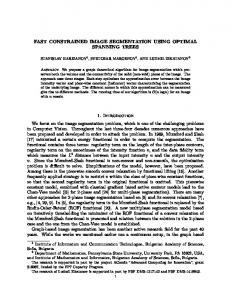
T Figure 3: The hidden Markov model on pixel label priors.
with θ by the EM algorithm. Translating the conditional independencies induced by the above graphical model, the penalized log-likelihood of the observed data reads (ignoring constants) L3 (θ, π) =
X i
log
K X k=1
p(yi |xi = k, θ)πik
K XXX (πik − πjk )2 . − β i
(18)
j∈Ni k=1
We note the similarity of L3 with the L1 of the standard mixture model. Here, however, there are n different πi distributions, one for each pixel i, and additionally there is a penalty term (the energy U ) that penalizes neighboring pixels to have similar labels. Note that this model enforces spatial dependences between pixels in a different way than the HMRF model of the previous section. Namely, here the assumption is that neighboring pixels have similar prior distributions that generate their pixel labels, whereas in the classical HMRF model we postulate a Markov random field directly on the pixel labels. An attractive property of this model, as we explain below, is that the E-step of the EM algorithm is easier to carry out since we do not need to estimate a restoration of the image. On the other hand, the M-step is more complicated as it also involves the penalty term −U (π) of (16). Indeed, the computational effort in [15, 16, 17] goes in the estimation of the {πi } priors in the M-step which requires solving a constrained P optimization problem (since πi is a discrete distribution with k πik = 1 for each i). The main motivation for using this model as opposed to the traditional MRF model on pixel labels (of Section 2.2), is its flexibility with respect to the initial conditions. This flexibility is manifested in the shape of the objective function; In the traditional MRF model of Section 2.2, the penalized log-likelihood function will be sharper and will contain several local maxima, and hence it will be more sensitive to the initial solution. In the current model, the field constraints are directly enforced over the parameters of the label priors, resulting in a smoother objective function. This can be intuitively seen by noting that distinct parameter values for some priors may induce exactly the same pixel labels, and therefore
6
An Efficient Spatially Constrained EM Algorithm for Image Segmentation
searching in the space of priors (in the M-step of our algorithm, see below) will be easier than searching in the space of labels. This search will be also facilitated by the fact that the space of prior parameters is continuous, as opposed to the discrete nature of the space of pixel labels. Interestingly, although the current model contains more parameters (Kn, a vector of K parameters for each πi , as opposed to n of the traditional MRF model), the smoothness of the objective function, as argued above, allows the result to be less dependent on the initialization. The above arguments will be experimentally verified in Section 4.
3 The Proposed Method In our method we also use the graphical model of Fig. 3, but we use a different modeling strategy for the spatial dependences between the priors and a different algorithm for learning the unknown parameters. As in [1] we employ the Besag approximation for modeling the joint density over pixel priors: Y p(πi |πNi , β), (19) p(π|β) ≈ i
where we define πNi as a mixture distribution over the priors of neighboring pixels of pixel i, i.e., X πNi = λij πj , (20) j∈Ni j6=i
P where λij are fixed positive weights and for each i holds j λij = 1. The mixing weight λij depends on the relative offset between the pixels i and j, while the mixture does not include the prior of the same pixel i. Note that the evaluation of this mixture corresponds to a convolution operation π·k ∗ λ, for each component k, where λ is a symmetric linear image filter with zero coefficient in its center and nonnegative coefficients elsewhere that sum to one. See Section 4.2 for more details about filter related issues. Further, for the conditional density p(πi |πNi , β) we assume a log-model in the form (ignoring constants) £ ¤ log p(πi |πNi , β) = −β D(si k πi ) + D(si k πNi ) + H(si ) (21) PK PK where, e.g., D(si k πi ) = k=1 sik log sik − k=1 sik log πik is the Kullback-Leibler divergence between si and πi (which is always nonnegative and becomes zero when si = πi ), and H(si ) = P s − K k=1 ik log sik is the entropy of the distribution si (which is always nonnegative and reaches its maximum when si is uniform). Note that the above log-prior (21) is parameterized by a discrete distribution si over components. If si = πi then (21) becomes £ ¤ log p(πi |πNi , β) = −β D(πi k πNi ) + H(πi ) (22) which intuitively expresses the degree of similarity between the prior of pixel i and the priors of its neighbors, and it provides a way of constraining neighboring pixels to have similar class labels. Similarly, the entropy term H(πi ) constrains the label priors to be as informative as possible: in homogeneous regions we want neighboring pixels to have similar priors, but we also want those priors to be far from uniform. The reason for defining our model constraints using (21) instead of the more intuitive model (22) is because (21) allows for an efficient coordinate ascent EM-like optimization, as we will show next. Since the log-prior penalty (21) involves only entropic quantities, it defines a lower bound to the data log-likelihood. We can further constrain our model by imposing a similar penalty involving posteriors, in the form ¤ 1£ − D(qi k pi ) + D(qi k pNi ) + H(qi ) (23) 2
Section 3
The Proposed Method
7
where qi is an arbitrary class distribution for pixel i, and pi is the posterior class distribution of a pixel i computed for model parameters θ and prior πi by the Bayes rule: p(yi |xi = k, θ)πik pik ≡ p(xi = k|yi , θ, πik ) = PK . l=1 p(yi |xi = l, θ)πil
(24)
The coefficient 1/2 in the penalty term above was chosen because it allows a tractable M-step as we show next. Putting all terms together, the penalized log-likelihood of the observed data as a function of the model parameters and the introduced auxiliary distributions s = {si } and q = {qi } reads (ignoring constants): X X log p(yi |xi = k, θ)πik F(θ, π, s, q) = i
k
¤ 1£ − D(qi k pi ) + D(qi k pNi ) + H(qi ) 2£ ¤ − β D(si k πi ) + D(si k πNi ) + H(si ) .
(25)
We note here that similar approaches to incorporate problem constraints by lower bounding the loglikelihood have also been suggested in [18, 19]. Our EM algorithm maximizes the energy F in (25) by coordinate ascent. In the E-step we fix θ and π and maximize F over s and q. In the M-step we fix s and q and maximize F over θ and π. Next we show how these two steps can be performed. E-step In the E-step we optimize over si for a pixel i, assuming θ and π fixed. A similar derivation holds for qi . The terms of F involving si are: X X X X X sik log sik = sik log πNi k + sik log sik + sik log πik − sik log sik + − −
sik log sik +
k
X
k
k
k
k
k
X
sik log(πik πNi k ).
(26)
k
The latter is an (un-normalized) negative KL-divergence which becomes zero when si ∝ πi πNi .
(27)
qi ∝ pi pNi .
(28)
Similarly we obtain
M-step In the M-step we fix s and q and maximize F over θ and π. We show here the derivation involving the posteriors pi . A similar derivation holds for the priors πi . The terms of F involving pi (and therefore θ and πi ) are: X X ¤ 1£ log p(yi |xi = k, θ)πik − D(qi k pi ) + D(qi k pNi ) + D(qj k pNj ) + H(qi ) (29) 2 j∈Ni j6=i
k
where the mixture pNj reads: pNj =
X
λjm pm
m∈Nj m6=j
= λji pi +
X m∈Nj m6=i,j
λjm pm .
(30)
8
An Efficient Spatially Constrained EM Algorithm for Image Segmentation
The above mixture pNj appears in the terms D(qj k pNj ) for all pixels j that are neighbors of pixel i. To make the M-step tractable, we bound these KL terms using Jensen’s inequality: X
log pNj ≥ λji log pi + (1 − λji ) log
m∈Nj m6=i,j
λjm pm . (1 − λji )
(31)
Collecting only terms that involve pi , and noting that λji = λij , we finally get: log
X
p(yi |xi = k, θ)πik +
k
1X 1X qik log pik + qNi k log pik 2 2 k
where the distribution qNi is qNi =
X
(32)
k
λij qj .
(33)
j∈Ni j6=i
Expanding the posterior pi in the above terms we immediately see that the log-likelihood term cancels. An identical derivation holds for P the priors πi . Collecting all terms and differentiating w.r.t. πi (using a Lagrange multiplier to ensure k πik = 1), we can easily show that we get: 1 πi = (qi + qNi ) + β(si + sNi ). 2
(34)
Similarly, differentiating F over θ and using the chain rule over i, we get the following update equations for the means and covariances of the K Gaussian components: P i (qi + qNi ) yi , (35) mk = P i (qi + qNi ) P (qi + qNi ) yi yi> Ck = iP − mk m> (36) k. (q + q ) i N i i Note that the update equations for θ are analogous to those in the standard mixture model, with the difference that here the weights correspond to ‘smoothed’ pixel posteriors. The use of such spatially smoothed weights in the M-step of the EM algorithm is a key element in our approach that distinguishes it from other works. The complete algorithm is shown in Alg. 1. Finally, in this work we set β = 0.5. It is a matter of future work to investigate ways to incorporate β in the optimization process (as in [1, 11]). 1: 2: 3: 4: 5: 6: 7: 8: 9: 10: 11: 12:
Initialize the parameter vector θ, e.g., using k-means. Initialize the priors {πi }, e.g., uniform πik = K1 , ∀i, k. E-step: Compute posterior probabilities pi using (24) and the current estimates of θ and {πi }. P Compute {si } according to (27) and (20) and normalize each sP so that s = 1. i k ik Compute {qi } according to (28) and normalize each qi so that k qik = 1. M-step: Update the parameter vector θ using (35) and (36). Update {πi } according to (34). Evaluate F from (25). If convergence of F, e.g., |Ft+1 /Ft − 1| < ² then stop. else go to step 3. end if Algorithm 1: The proposed EM algorithm for image segmentation
Section 4
Experiments
9
4 Experiments In this section we demonstrate the performance of our algorithm on synthetic and real images. Specifically, in Section 4.1 we evaluate the performance of our segmentation algorithm in the presence of noise. Section 4.2 includes additional experiments to test the algorithm’s behavior w.r.t the choice of parameters and initialization. Section 4.3 presents segmentation results on gray level images. Finally, in Section 4.4 we show segmentation results on color images.
4.1 Noise-Corrupted Synthetic Images We first illustrate our algorithm on synthetic images and consider its robustness against noise. We use the same synthetic images as in [12, 17]. These are simulated three-class and five-class images (see Fig. 4(a) and Fig. 5(a)) sampled from an MRF model using the Gibbs sampler [20]. In Fig. 4(b) and Fig. 5(b) we show the same images after adding white Gaussian noise with σ = 52. In Fig. 4(c) and Fig. 5(c) we show the segmentation results of the standard EM algorithm using the generative model discussed in Section 2.1. It is clear from these examples that in presence of noise, an algorithm that does not use spatial constrains cannot produce meaningful segmentation results. On the contrary, a method like ours that does take into account the spatial relation of pixels can successfully segment these noisy images, as we demonstrate in Fig. 4(g) and Fig. 5(g). The total running time of our method (from initialization till convergence) was 15 seconds for the image shown in Fig. 4(g) and 92 seconds for the one shown in Fig. 5(g). All times (for our method) refer to a Matlab implementation running on a 3.0GHz PCbased workstation. In these synthetic images the ground truth is known (the true assignment of pixels to the K classes), which allows us to evaluate the performance of the various methods in terms of the misclassification ratio (MCR). This is simply the number of misclassified pixels divided by the total number of pixels [12]. We compare our method with related methods based on hidden Markov random fields: the ICM algorithm [14] (termed ICM); the Spatially Variant Finite Mixture Model method [15] (termed SVFMM); the extension to SVFMM [17] (termed SVFMM-QD); the Hidden Markov Random Field Model based on EM framework proposed in [12] (termed HMRF-EM); the Mean field and the Simulated field methods of [1, 10] (termed MeanF and SimF respectively). Finally, we have also included the comparison with the standard EM algorithm. Tables 1 and 2 contain the misclassification ratio results of the previously mentioned methods for the same synthetic images and for various amounts of noise. For the methods SVFMM, SVFMM-QD and HMRF-EM we replicate the misclassification ratio results reported in the corresponding papers. For SimF and MeanF methods we used a software implementation developed by the authors of [1, 10] (in C) and is publicly available at http://mistis.inrialpes.fr/software/SEMMS.html. This software also includes an implementation of the ICM algorithm. We initialize ICM, SimF and MeanF methods in the same way that we initialize our algorithm. As in [1, 10] the number of iteration for SimF and MeanF was set to 100 and the ICM was run until convergence. For our method the restorations shown result from the maximization of the estimated prior distribution πi (which the algorithm learns). The experiments point out that in all methods the misclassification ratio increases as the amount of noise and the number of labels K increases. Our method performs much better than all other methods when moderate or high amount of noise is present, and it is competitive to other methods for low amounts of noise. Our method, implemented in Matlab, was faster than SimF and MeanF methods, which were implemented in C and optimized. In Fig. 4 and Fig. 5 we present the running time and the segmentation results of ICM, SimF and MeanF methods for the three-class and five-class image respectively.
4.2 Choice of Parameters Our algorithm has in total three parameters, the number of components K, the priors parameter β, and the image filter used in (20). In this work we assume that the number of components K as well as the
10
An Efficient Spatially Constrained EM Algorithm for Image Segmentation
(a)
(b)
(c)
(d)
(e)
(f)
(g)
Figure 4: Synthetic image with three classes. (a) The original image. (b) The noise corrupted image
with additive white Gaussian noise (σ = 52). (c) The segmentation result of the standard EM algorithm (MCR 23.9%). (d) The segmentation result of ICM with running time of 10 sec (MCR 0.96%). (e) The segmentation result of SimF with running time of 65 sec (MCR 0.59%). (f) The segmentation result of MeanF with running time of 60 sec (MCR 0.54%). (g) The segmentation result of our approach with running time of 15 sec (MCR 0.50%).
Section 4
Experiments
11
(a)
(b)
(c)
(d)
(e)
(f)
(g)
Figure 5: Synthetic image with five classes. (a) The original image. (b) The noise corrupted image
with additive white Gaussian noise (σ = 52). (c) The segmentation result of the standard EM algorithm (MCR 53.7%). (d) The segmentation result of ICM with running time of 39 sec (MCR 31.7%). (e) The segmentation result of SimF with running time of 90 sec (MCR 2.88%). (f) The segmentation result of MeanF with running time of 100 sec (MCR 3.89%). (g) The segmentation result of our approach with running time of 92 sec (MCR 1.78%).
12
An Efficient Spatially Constrained EM Algorithm for Image Segmentation
Table 1: Misclassification results for the three-class image.
HMRF-EM SVFMM-QD SVFMM EM ICM SimF MeanF Our Approach run time of our approach
18 0.1% 0.2% 0.61% 0.03% 0.02% 0.02% 0.03% 5.8 sec
Noise σ 28 47 0.12% 1.04% 5.82% 20.5% 0.21% 0.81% 0.13% 0.43% 0.12% 0.39% 0.1% 0.46% 8.8 sec 14 sec
52 13% 21% 23.9% 0.96% 0.62% 0.54% 0.50% 15 sec
95 8.73% 42.3% 4.01% 1.52% 1.32% 1.18% 29 sec
Noise σ 25 33 1.36% 10% 30% 28.2% 43.1% 1.24% 4.44% 0.47% 0.92% 0.49% 0.73% 0.49% 0.73% 27 sec 40 sec
47 7.68% 53.8% 24.6% 2.19% 2.41% 1.49% 76 sec
52 28% 42% 53.7% 31.7% 2.88% 3.89% 1.78% 92 sec
25 1% 1.5% 3.64% 0.15% 0.08% 0.08% 0.1% 7.7 sec
Table 2: Misclassification results for the five-class image.
HMRF-EM SVFMM-QD SVFMM EM ICM SimF MeanF Our Approach run time of our approach
18 4% 6% 15.1% 0.47% 0.26% 0.23% 0.24% 19 sec
23 0.2% 27.1% 0.94% 0.46% 0.38% 0.39% 23 sec
Section 4
Experiments
13
observation model family are given to us for a particular image. Also, in experiments not shown here we determined that 0.5 is a good choice for the parameter β. As already mentioned, it is a matter of future work to investigate ways to incorporate this parameter in the optimization process. In this section we will consider the only other free parameter in our algorithm which is the filter used for evaluating the mixtures πNi , pNi , qNi and sNi (see Eq. (20) and Eq. (33)). Specifically, as mentioned in Section 3 the evaluation of such mixtures can be achieved by convolving with an image filter. In order for these mixtures to be valid distributions (without the need of extra normalization) the applied filter must have coefficients that sum to one. Our algorithm also requires that the center coefficient of the filter be zero. Also, we choose the filter to be symmetric. In the case where domain knowledge would imply some (simple) spatial relation between pixels with the same class label, this knowledge could be easily incorporated into our framework by employing a non symmetric filter that encourages these spatial relations. Clearly the choice of filter can affect the performance of the algorithm and the quality of the segmentation. In addition the mixture calculation can be performed by a variety of images filters. In the previous section we presented the results of our algorithm that were achieved using a ‘modified’ (i.e. the center coefficient set to zero) pillbox filter with diameter δ equal to 5. In Table 3 we report the misclassification ratio results using different filters for the three class image (see Fig. 6(a)), after adding white Gaussian noise with σ = 95 (see Fig. 6(b)). We used ‘modified’ versions (i.e. the center coefficient is set to zero) of a low pass Gaussian filter and a mean filter. In Fig. 6(c) we show the corresponding segmentation results for Gaussian filters with σ = 1. The results illustrate that a larger filter size can compensate for the presence of high noise levels in the image. A closer look at Fig. 6(a),(c) reveals that large size filters, while providing increased robustness to noise, tend to oversmooth the edges. When the noise levels in an image are low there is no benefit from using large size filters, and the resulting oversmoothing of the edges just decreases the segmentation accuracy. Clearly, if the noise level of images in a particular domain is known a priori, then the filter type and its parameters can be fine-tuned for optimal performance.
(a)
(b)
(c)
Figure 6: The effects of using different filters on the segmentation results. (a) The original 3-class im-
age. (b) The noise corrupted image with additive white Gaussian noise of σ = 95. (c) The segmentation result using Gaussian kernel with σ = 1 (MCR 1.08%).
Table 3: Misclassification results for Fig. 6(b) with different filters.
Gaussian (σ = 0.5) 1.19%
Gaussian (σ = 1) 1.08%
mean 3 × 3 1.23 %
mean 5 × 5 1.16%
14
An Efficient Spatially Constrained EM Algorithm for Image Segmentation
4.3 Gray-Level Images In natural images a number of difficult aspects of image segmentation come together, like noise and varying imaging conditions. Additionally, the true value of image labels K is not known. In the following experiments we use the same images as in [21, 22, 10] where K was estimated using (approximations of) the Bayesian Information Criterion (BIC). Fig. 7(a) shows a 128 × 128 Positron Emission Tomography (PET) image of a dog lung and Fig. 8(a) shows an aerial 100×100 image of a buoy against a background of dark water (see [21] for more details on their nature and origin). For the PET image of a dog lung the image’s labels K was estimated to be 3. In Fig. 7(c)-(f) we demonstrate the segmentation results of ICM, MeanF, SimF and our approach. For our method we used a ‘modified’ (i.e. the center coefficient set to zero) pillbox filter with diameter δ equal to 7. All other settings for all methods were the same as in Section 4.1. All algorithms were initialized by a simple thresholding of the image as shown in Fig. 7(b). The result shows that MeanF, SimF and our approach perform approximately the same and are producing more homogeneous regions for the lungs than the ICM algorithm. For the buoy image the image’s labels K was estimated to be 3. In Fig. 8(d)-(g) we demonstrate the segmentation results of ICM, MeanF, SimF and our approach. We used the same settings for all methods as in Section 4.1. All algorithms were initialized using the k-means based initialization which is shown in Fig. 8(b). It is clear that all algorithms given this particular initialization perform approximately the same and they are all capable of correctly assigning the pixels belonging to the buoy to one cluster. In Fig. 8(h)-(k) we show the segmentation results of the four methods using the same setting as before but employing an alternative initialization based on EM for independent mixtures. This initialization is shown in Fig. 8(c), where the horizontal scan lines from the imaging process of Fig. 8(a) can be clearly observed. Only our approach was able to correctly assign the pixels belonging to the buoy to one cluster given this EM based initialization. The buoy experiment demonstrates a significant aspect of our approach, namely, that it is relatively insensitive to initialization compared to other methods. We feel that this is an important aspect, since in natural images, not only the true value of image labels K is hard to estimate, but also an appropriate initialization cannot be known a priori.
4.4 Color Images In Fig. 9–11 we show the segmentation results of three different color images from the Berkeley Segmentation Dataset [23]. In all three figures, we show the original image, the initializations obtained by K-means and EM, the results of our method with these two initializations, and the corresponding results of ICM, SimF and MeanF. In all three examples our algorithm is able to consistently segment the original image independently of the initialization, whereas all three HMRF-based methods are rather sensitive to the initial conditions. The reasons for choosing a Gaussian observation model over more elaborated alternatives (i.e., the FRAME model [2]) that can model is that In Fig. 12 we show the segmentation results of an image in rgb color space when the Gaussian observation model assumption is violated. Normalized rgb color (chromaticity) has been widely used by many researchers in the field of image segmentation, e.g. [24, 25], because of its important invariant properties. Specifically, it has been shown in [26] that, under the assumption of the dichromatic reflection model, normalized color is to a large extent invariant to a change in camera viewpoint, object pose, and the direction and intensity of the incident light. In addition, the color transformation from RGB to normalized color rgb is simple and easy to compute. Namely, based on the measured RGB-values,
Section 4
Experiments
15
(a)
(b)
(c)
(d)
(e)
(f)
Figure 7: Segmentation example of the PET image of a dog lung with K = 3. (a) The original image. (b) Simple thresholding based initialization. (c) The segmentation result of ICM. (d) The segmentation result of SimF. (e) The segmentation result of MeanF. (f) The segmentation result of our approach.
normalized color rgb is computed as follows: r = R/(R + G + B)
(37)
g = G/(R + G + B)
(38)
b = B/(R + G + B)
(39)
However, this (non-linear) color transformation has a serious drawback, as it becomes unstable for some RGB sensor values. Particularly, rgb is undefined at the black point (R = G = B = 0) and is unstable near this singular point. As a consequence, a small perturbation for dark (low-intensity) sensor values (e.g. due to sensor noise), will cause a significant jump in the transformed values. To be precise, under the assumption that the sensor noise is normally distributed, the uncertainty for rgb are computed as follows: [27]: s σr = s σg =
2 + σ 2 ) + (G + B)2 σ 2 R2 (σB G R (R + G + B)4
2 + σ 2 ) + (R + B)2 σ 2 G2 (σB R G , (R + G + B)4
(40)
where σR , σG , and σB are the noise estimates for the RGB-values in the image. A standard way to calculate the standard deviations σR , σG , and σB is to compute the mean and variance estimates derived from a white surface patch in the image under controlled imaging conditions (i.e. diffuse reflection and uniform lighting). From the analytical study of (40), it can be derived that normalized color becomes unstable around the black point R = G = B = 0. In Fig. 12(b), which is the normalized rgb color transformation of Fig. 12(a), the unstable invariant values are clearly visible at the bottom of the red ball. The presence of these unstable invariant values violate the assumed Gaussian observation model. Fig. 12(c)-(e) show the segmentation results for K = 6
16
An Efficient Spatially Constrained EM Algorithm for Image Segmentation
(a)
(b)
(c)
(d)
(e)
(f)
(g)
(h)
(i)
(j)
(k)
Figure 8: Segmentation example of the buoy image with K = 3. (a) The original image. (b) K-means
initialization. (c) Initialization based on EM for independent mixtures. (d) The segmentation result of ICM with k-means initialization. (e) The segmentation result of SimF with k-means initialization. (f) The segmentation result of MeanF with k-means initialization. (g) The segmentation result of our approach with k-means initialization. (h) The segmentation result of ICM with EM initialization. (i) The segmentation result of SimF with EM initialization. (j) The segmentation result of MeanF with EM initialization. (k) The segmentation result of our approach with EM initialization.
Section 4
Experiments
(a)
17
(b)
(c)
(d)
(e)
(f)
(g)
(h)
(i)
(j)
(k)
Figure 9: Segmentation example of the water buffalo image with K = 2. (a) The original image.
(b) K-means initialization. (c) The segmentation result of our approach with k-means initialization. (d) Initialization based on EM for independent mixtures. (e) The segmentation result of our approach with EM initialization. (f) The segmentation result of ICM with k-means initialization. (g) The segmentation result of SimF with k-means initialization. (h) The segmentation result of MeanF with k-means initialization. (i) The segmentation result of ICM with EM initialization. (j) The segmentation result of SimF with EM initialization. (k) The segmentation result of MeanF with EM initialization.
18
An Efficient Spatially Constrained EM Algorithm for Image Segmentation
(a)
(b)
(c)
(d)
(e)
(f)
(g)
(h)
(i)
(j)
(k)
Figure 10: Segmentation example of the rock garden image with K = 2. (a) The original image. (b) K-means initialization. (c) The segmentation result of our approach with k-means initialization. (d) Initialization based on EM for independent mixtures. (e) The segmentation result of our approach with EM initialization. (f) The segmentation result of ICM with k-means initialization. (g) The segmentation result of SimF with k-means initialization. (h) The segmentation result of MeanF with k-means initialization. (i) The segmentation result of ICM with EM initialization. (j) The segmentation result of SimF with EM initialization. (k) The segmentation result of MeanF with EM initialization.
Section 4
Experiments
(a)
19
(b)
(c)
(d)
(e)
(f)
(g)
(h)
(i)
(j)
(k)
Figure 11: Segmentation example of the dog sled image with K = 3. (a) The original image. (b) K-
means initialization. (c) The segmentation result of our approach with k-means initialization. (d) Initialization based on EM for independent mixtures. (e) The segmentation result of our approach with EM initialization. (f) The segmentation result of ICM with k-means initialization. (g) The segmentation result of SimF with k-means initialization. (h) The segmentation result of MeanF with k-means initialization. (i) The segmentation result of ICM with EM initialization. (j) The segmentation result of SimF with EM initialization. (k) The segmentation result of MeanF with EM initialization.
20
An Efficient Spatially Constrained EM Algorithm for Image Segmentation
for the normalized color image of Fig. 12(b) with ICM, SimF and MeanF, respectively. In Fig. 12(f) we show the corresponding results with our approach. All figures show a reconstruction of the normalized rgb image, with pixel values in the final result corresponding to the estimated mean of their assigned Gaussian component. The results show that our approach produces more homogeneous regions than other algorithms and consequently a better segmentation.
(a)
(b)
(c)
(d)
(e)
(f)
Figure 12: Segmentation example of a color image with K = 6. (a) The original image. (b) The normalized rgb color image. (c) The segmentation result of ICM in rgb color space. (d) The segmentation result of SimF in rgb color space. (e) The segmentation result of MeanF in rgb color space. (f) The segmentation result of our approach in rgb color space.
5 Conclusions We proposed a graphical model and a novel EM algorithm for Markov-based image segmentation. The proposed model postulates that the unobserved pixel labels are generated by prior distributions that have similar parameters for neighboring pixels. The proposed EM algorithm performs iterative bound optimization of a penalized log-likelihood of this model. The derived EM equations are similar to the standard (unconstrained) EM algorithm, with the only difference that a ‘smoothing’ step is interleaved between the E- and the M-step, that couples the posteriors of neighboring pixels in each iteration. Compared to other Markov-based algorithms for segmentation, our algorithm is very simple to implement, while experimental results have demonstrated that it is very competitive to state-of-the-art methods in terms of speed and solution quality.
REFERENCES
21
References [1] G. Celeux, F. Forbes, and N. Peyrard, “EM procedures using mean field-like approximations for Markov model-based image segmentation,” Pattern Recognition, vol. 36, no. 1, pp. 131–144, 2003. [2] S. C. Zhu, Y. Wu, and D. Mumford, “Filters, random fields and maximum entropy (FRAME): Towards a unified theory for texture modeling,” Intern. Journal of Computer Vision, vol. 27, no. 2, pp. 107–126, 1998. [3] G. McLachlan and D. Peel, Finite Mixture Models. John Wiley & Sons Inc, November 2000. [4] C. Carson, S. Belongie, H. Greenspan, and J. Malik, “Blobworld: Image segmentation using Expectation-Maximization and its application to image querying,” IEEE Trans. on Pattern Analysis and Machine Intelligence, vol. 24, no. 8, pp. 1026–1038, 2002. [5] A. Diplaros, T. Gevers, and N. Vlassis, “Skin detection using the EM algorithm with spatial constraints,” in IEEE International Conference on Systems, Man and Cybernetics, The Hague, Netherlands, 2004. [6] A. Dempster, N. Laird, and D. Rubin, “Maximum likelihood from incomplete data via the EM algorithm,” Journal of the Royal Statistical Society. Series B (Methodological), vol. 39, no. 1, pp. 1–38, 1977. [7] R. Neal and G. Hinton, “A view of the EM algorithm that justifies incremental, sparse, and other variants,” in Learning in Graphical Models, M. Jordan, Ed. Kluwer Academic Publishers, 1998, pp. 355–368. [8] W. Qian and D. M. Titterington, “Estimation of parameters in hidden Markov models,” Phil. Trans. R. Soc. A, vol. 337, pp. 407–428, 1991. [9] J. Zhang, “The mean field theory in EM procedures for Markov random fields,” IEEE Trans. Signal Process., vol. 40, no. 10, pp. 2570–2583, 1992. [10] F. Forbes and N. Peyrard, “Hidden Markov random field model selection criteria based on mean field-like approximations,” IEEE Trans. on Pattern Analysis and Machine Intelligence, vol. 25, no. 9, pp. 1089–1101, 2003. [11] J. Sun and D. Gu, “Bayesian image segmentation based on an inhomogeneous hidden markov random field,” in 17th International Conference on Pattern Recognition (ICPR 2004), vol. 1, 2004, pp. 596–599. [12] Y. Zhang, M. Brady, and S. Smith, “Segmentation of brain MR images through a hidden Markov random field model and the Expectation-Maximization algorithm,” IEEE Trans. on Medical Imaging, vol. 20, no. 1, pp. 45–57, January 2001. [13] J. Besag, “Statistical analysis of non-lattice data,” The Statistician, vol. 24, no. 3, pp. 179–195, 1975. [14] ——, “On the statistical analysis of dirty pictures,” Journal of the Royal Statistical Society. Series B (Methodological), vol. 48, no. 3, pp. 259–302, 1986. [15] S. Sanjay-Gopal and T. J. Hebert, “Bayesian pixel classification using spatially variant finite mixtures and the generalized EM algorithm,” IEEE Trans. on Image Processing, vol. 7, no. 7, pp. 1014–1028, 1998.
22
REFERENCES
[16] J. L. Marroquin, E. A. Santana, and S. Botello, “Hidden Markov measure field models for image segmentation,” IEEE Trans. on Pattern Analysis and Machine Intelligence, vol. 25, no. 11, pp. 1380–1387, 2003. [17] K. Blekas, A. Likas, N. Galatsanos, and I. E. Lagaris, “A spatially-constrained mixture model for image segmentation,” IEEE Transactions on Neural Networks, vol. 16, no. 2, pp. 494–498, 2005. [18] S. T. Roweis, L. K. Saul, and G. E. Hinton, “Global coordination of local linear models,” in Advances in Neural Information Processing Systems 14 (NIPS’01), T. G. Dietterich, S. Becker, and Z. Ghahramani, Eds. Cambridge, MA: MIT Press, 2002, pp. 889–896. [19] J. J. Verbeek, N. Vlassis, and B. Kr¨ose, “Self-organizing mixture models,” Neurocomputing, vol. 63, pp. 99–123, 2005. [20] S. Geman and D. Geman, “Stochastic relaxation, Gibbs distributions, and the Bayesian restoration of images,” IEEE Trans. on Pattern Analysis and Machine Intelligence, vol. 6, pp. 721–741, 1984. [21] D. C. Stanford, “Fast automatic unsupervised image segmentation and curve detection in spatial point patterns,” Ph.D. dissertation, University of Washington Statistics Department, 1999. [22] D. C. Stanford and A. E. Raftery, “Approximate Bayes Factors for image segmentation: The Pseudolikelihood Information Criterion (PLIC),” IEEE Trans. on Pattern Analysis and Machine Intelligence, vol. 24, no. 11, pp. 1517–1520, 2002. [23] D. Martin, C. Fowlkes, D. Tal, and J. Malik, “A database of human segmented natural images and its application to evaluating segmentation algorithms and measuring ecological statistics,” in Eighth IEEE International Conference on Computer Vision, vol. 2, July 2001, pp. 416–423. [24] G. Healey, “Segmenting images using normalized color,” IEEE Trans. on Systems, Man, and Cybernetics, vol. 22, no. 1, pp. 64–73, 1992. [25] T. Gevers, “Adaptive image segmentation by combining photometric invariant region and edge information,” IEEE Trans. on Pattern Analysis and Machine Intelligence, vol. 24, no. 6, pp. 848– 852, 2002. [26] T. Gevers and A. W. M. Smeulders, “Color-based object recognition,” Pattern Recognition, vol. 32, no. 3, pp. 453–464, 1999. [27] T. Gevers and H. Stokman, “Robust histogram construction from color invariants for object recognition,” IEEE Trans. on Pattern Analysis and Machine Intelligence, vol. 26, no. 1, pp. 113–117, 2004.
Acknowledgements The authors are thankful to D. Barber, K. Blekas, A. T. Cemgil, N. Galatsanos, I. Patras, C. Veenman and J. J. Verbeek for their valuable comments. The authors are grateful to N. Peyrard for making publicly available the implementation of MeanF, SimF and ICM methods. This work is an IOP project sponsored by the Dutch Ministry of Economic Affairs, project number IBV99001.
IAS reports This report is in the series of IAS technical reports. The series editor is Stephan ten Hagen (
[email protected]). Within this series the following titles appeared: J.J. Verbeek Rodent behavior annotation from video. Technical Report IAS-UVA-0502, Informatics Institute, University of Amsterdam, The Netherlands, November 2005. J.J. Verbeek and N. Vlassis. Semi-supervised learning with gaussian fields. Technical Report IAS-UVA-05-01, Informatics Institute, University of Amsterdam, The Netherlands, Februari 2005. J.M. Porta, M.T.J. Spaan, and N. Vlassis. Value iteration for continuous-state POMDPs. Technical Report IAS-UVA-04-04, Informatics Institute, University of Amsterdam, The Netherlands, December 2004. All IAS technical reports are available for download at the IAS website, http://www. science.uva.nl/research/ias/publications/reports/.