An Incremental Editor for Dynamic Hierarchical Drawing of Trees David Workman 1 , Margaret Bernard
2
, Steven Pothoven3
1
University of Central Florida, School of EE and Computer Science
[email protected] 2 The University of the West Indies , Dept. Math. & Computer science
[email protected] 3 IBM Corporation, Orlando, Florida
Abstract. We present an incremental tree editor based on algorithms for manipulating shape functions. The tree layout is hierarchical, left-to-right. Nodes of variable size and shape are supported. The paper presents algorithms for basic tree editing operations, including cut and paste. The layout algorithm for positioning child-subtrees rooted at a given parent is incrementally recomputed with each edit operation; it attempts to conserve the total display area allocated to child-subtrees while preserving the user’s mental map. The runtime and space efficiency is good as a result of exploiting a specially designed Shape abstraction for encoding and manipulating the geometric boundaries of subtrees as monotonic step functions to determine their best placement. All tree operations, including loading, saving trees to files, and incremental cut and paste, are worst case O(N) in time, but typically cut and paste are O(log(N)2), where N is the number of nodes.
1 Introduction Effective techniques for displaying static graphs are well established but in many applications the data are dynamic and require special visualization techniques. Applications arise when the data are dynamically generated or where there is need to interact with and edit the drawing. Dynamic techniques are also used for displaying large graphs where the entire graph cannot fit on the screen. In this paper, we present an incremental tree editor, DW-tree, for dynamic hierarchical display of trees. Graphs that are trees are found in many applications including Software Engineering and Program Design, which is the genesis of this Dynamic Workbench DW-tree software [5, 1, 4]. DW-tree is an interactive editor; it allows users to interact with the drawing, changing nodes and subtrees. In redrawing the tree after user changes, the system reuses global layout information and only localized subtree data need to be updated. A full complement of incremental editing operations is supported, including changing node shape and size as well as cutting and pasting subtrees. The editor has the capability of loading (saving) a tree from (to) an external file . The tree editor uses Shape vectors for defining the boundary of tree or subtree objects. Incremental tree editing operations are based on algorithms for manipulating Shape vectors. The tree layout is hierarchical, left -to-right (horizontal). The DW-tree drawing algorithms attempt to conserve the total display area allocated to child-subtrees (area efficient) without appreciably distracting the user’s mental continuity upon re-display. For a tree of size N nodes, the runtime efficiency is O(N) for load and save operations to an external file. For cut and paste operations at depth d, under reasonable assumptions, the runtime is O(d 2 ), with d = log(N).
Page 1
The remainder of the paper is organized as follows. First (Section 2), we present the principles for tree layout using the Shape abstraction. In section 3, we present key principles and algorithms that form the basis for the incremental editor operations and in Section 4 we discuss related work; we close with some concluding remarks in section 5.
2 Tree Layout Principles In this section we present the layout design principles and definitions that provide the conceptual foundation and framework for the remainder of the paper. The display area of the editor defines a 2D coordinate system as depicted in Figure 1. Coordinate values along both axes are multiples of the width (fduW) and height (fduH) of the Fundamental Display Unit (FDU), the smallest unit of display space allocated in the horizontal and vertical directions, respectively.
Figure 1. Display Coordinate System,Tree Layout, and Bounding Shape Functions.
Nodes can be of any size, but are assumed to occupy a display region bounded by a rectangle having width and height that are multiples of fduW and fduH, respectively. The absolute display coordinates of a node are associated with the upper left corner of its bounding rectangle. Trees are oriented left-to-right as shown in Figure 1, where the Parent node and its First Child always have the same vertical displacement. All children with the same parent node have the same relative horizontal displacement, Hspc. If (x,y) denotes the FDU coordinates of a parent node, and the parent node has width (Pwidth) and height (Pheight), then the coordinates of child node, k, will always be (x + Pwidth + Hspc, y + ∆k ), where for 1 ≤ k ≤ Nchildren, ∆1 = 0, and for k > 1, ∆k = ∆(k-1) + Cheight (k-1) + Vspc. Vspc is the minimum vertical separation between children. The actual vertical separation between children of the same parent is defined by our layout algorithms to conserve display area and
Page 2
will be presented in a later section entitled, Tree Operations. H denotes the vertical displacement of all children (H = ∆Nchildren + Cheight Nchildren ). Edges are represented as polygonal lines in which the segments are either horizontal or vertical (orthogonal standard). An edge from parent to first child is a horizontal line. Edges from parent to other children have exactly two bends and consist of horizontal-vertical-horizontal segments. The edges from a parent to all its children overlap to form a ‘trunk’. To allow space for edge drawings, each node is allocated an additional Hspc to its right in the horizontal direction. The rectangular region of width Hspc and height H, located at coordinates (x + Pwidth, y), is used by the parent node to draw the edges to all its children. An example of a trees drawn by the DW-tree editor is illustrated by Figure 2.
Figure 2. Screen Image of DWtree Editor. 2.1 Shape Functions Shape functions are objects that define the outline of a tree or subtree. Figure 1 illustrates the concept for some tree, T. The solid upper line outlines the upper shape (UT ) of T, the solid lower line outlines the lower shape (LT ) of T. The subtree rooted at a given node has relative coordinates (0, 0) and corresponds to the coordinates of its root node. Every such subtree, T, has a bounding rectangle of width WT and height HT; in Figure 1, WT = 20 and HT = 12. The width of a subtree always takes into
Page 3
account the horizontal spacing (Hspc) associated with the node(s) having maximum extent in the X direction. The upper shape function, UT, is a step function of its independent variable, x. We represent UT as a vector of pairs: UT = , where δxk = 1 denotes the length of the k th step, 1= k = n, and y 1 = 0. y k gives the value of the function in the kth step (interval). Along the X-axis the kth step defines a half-open k
interval [xk-1 , xk ) where
x 0 = 0 and x k = ∑ δx j . The width of T then becomes j =1
W T = xn – the right extreme of the last step interval of UT. Finally, we define steps(UT) ={x0 , x1 ,…, xn }, the set of interval end-points defined by UT, and dom(UT ) = [x0 , WT], the closed interval defined by the extreme X-coordinates of the minimal bounding rectangle for T. The lower shape function, LT , is defined in an analogous way with the roles of x and y reversed. That is, we represent LT as a step function with y as the independent variable. Specifically, for some m = 1, LT = < (x1 , δy 1 ), … (xm, δy m)>. Along the Y-axis the kth step defines a half-open interval [y k-1 , yk ) k
where
y 0 = 0 and y k = ∑ δy j . Thus the height of T becomes HT = ym – the right j =1
extreme of the last step interval of LT. And, we define steps(LT) = { y0 , y1 , …, ym }, the set of interval end-points defined by LT , and dom(LT ) = [y 0 , HT], the closed interval defined by the extreme Y-coordinates of the minimal bounding rectangle for T. Because of our layout conventions, the key step in our layout algorithm requires computing the vertical separation of adjacent siblings in a given subtree. Since the lower shape function and upper shape function are based on different independent variables, we must convert the lower shape function to an equivalent step function with x as the independent variable. We let Λ T denote the lower shape function of T where x is the independent variable. ΛT = < (δx1 , y1 ), … (δxm, ym)>, where δxk = (xk+1 – xk ) and yk are computed from LT as defined above. However, because xm+1 is not defined in LT we compute δxm = (W T – xm). As we will show later, it will always be the case that W T > xm, where xm is always taken from the last step interval of LT . 2.2 The Shape Algebra Incremental tree editing operations are based on algorithms for manipulating shape functions. As the basis for these algorithms, we introduce a simple algebra for manipulating shape functions. Each will be defined for upper shape functions – analogous definitions apply to lower shape functions (LT and ΛT ). UShape(dx ,y ) = an upper step function = . Similarly, LShape( x, dy ) = . UShape and LShape are distinct function types. Min(R,S) = Z, where R,S and Z are UShape functions. Assume that dom(R) ⊆ dom(S). Then dom(Z) = dom(S) and steps(Z) = steps(R) ∪ steps(S) for each x∈ steps(Z), Z(x) = min(R(x),S(x)), if x ∈ dom(R) ∩ dom(S); Z(x) = S(x), if x ∈ dom(S) – dom(R). Diff(R,S) = Z, where R,S and Z are UShape functions. Then dom(Z) = dom(R) ∩ dom(S) and steps(Z) = (steps(R) ∪ steps(S)) ∩ dom(Z). Finally, for each x∈
Page 4
steps(Z), Z(x) = R(x)-S(x). ScalarAdd(c, R) = ScalarAdd(R,c) = Z, where R and Z are UShape functions and c is a scalar constant. Z(x) = R(x)+c, for all x∈ dom(Z) = dom(R). In effect, the scalar c is added to the y-component (dependent variable) of each step in a UShape, and added to the x-component of each step in an LShape. Note: steps(Z) = steps(R). Cat(R,S) = Z, where R, S and Z are UShape functions. steps(Z) = { x | x∈ steps(R) or x = x’+WR , for x’∈ steps(S) } – {WR | y-value of the last step of R = y-value of the first step of S}, and dom(Z) = [0, WR +WS ]; Z(x) = R(x), if x ∈ dom(R); Z(x) = S(x’), if x = x’+ WR , where x’∈ dom(S). MaxElt(R) = C, where R is an UShape function. C = Max{ R(x) | x∈ dom(R)} = Max{ R(x) | x∈ steps(R)}. For Min(R,S) the runtime is O(|R|+|S|), where |R| denotes the number of steps in R (analogously of S). For ScalarAdd(R), MaxElt(R) the runtime is O( |R| ). For Cat(R, S) the runtime can be O(1) if linked structures are used to represent shape functions.
3 Tree Operations Some of the most basic operations on trees are: (Op-1) Create and edit a selected node. (Op-2) Cut and paste a subtree. (Op-3) Read (write) a tree from (to) an external file. (Op-4) Select a node in a tree. (Op 1) Creating/editing a node involves defining/changing the size of the bounding rectangle enclosing the node’s display image. This means (re-)computing the shape functions for the node and then propagating these changes throughout the rest of the tree in which the node is embedded. As this is a special case of cutting/pasting a subtree, we describe how shape functions are defined for a single node and defer the rest of the discussion to the subtree cutting/pasting operation, Op-2. If R is a free-standing node with width (R.width) and height (R.height), then: UR = UShape(R.width + Hspc, 0) and LR = LShape(0, R.height ). This is an O(1) operation. (Op-2) Cutting/Pasting a node. Let S and T be fully defined free-standing trees. We consider the operation of pasting S into T at some position. The position in T is a node previously identified through a select operation (Op-4). Let P denote the selected node in T and let R = root(S) denote the root of the tree S. The paste operation requires a parameter that defines the new relationship P is to have with respect to R in the composite tree, that is: R can be an upper/lower sibling of P (assuming P ≠ root(T)); R can be the (new)(only) first/last child of P. We describe the case where R is to become a new lower sibling of P. The other variations differ only in minor details. Figure 3 illustrates the trees S and T before and after the paste operation, respectively. The relevant shape functions are presented in the accompanying table. There are three key sub-algorithms incorporated in the algorithm for a complete Cut or Paste operation. Algorithm 1 (Change Propagation): If P is the parent of some node (child subtree) whose shape changes, then the shape functions for P (for the subtree rooted at P) must be recomputed (See Algorithms 2 and 3). No additional change is necessary
Page 5
to the shape functions of any other child of P. Once the shape functions for P have been recomputed, then this algorithm is repeated at the parent of P, etc., terminating only when the root of the tree is reached. The worst case running time is O(N), where N is the number of nodes in a tree. The worst case would occur with trees where every node has a single child. However, if we assume a randomly chosen tree with N nodes, then the tree will tend to be balanced – each node has approximately the same number of children, say b. Thus Change Propagation will require O(dp) running time, where d denotes the depth in the tree where the first change occurs ( d ≈ logb (N)) and p denotes the worst case running time at each level on a path to the root. The running time at each level is essentially the running time of Algorithm 2 and 3 combined.
Figure 3. Subtree Paste Operation. Tree (Figure 3) T before paste S before paste T after paste
Upper Shape (U)
Lower Shape (L) < (0,2), (4,7) > < (0,2), (7, 4) > < (0,2), (4, 10), (11, 1 ) >
Lower Shape (Λ) < (4,2), (9,7) > < (7,2), (5,4) > < (4,2), (7, 10), (5, 1 ) >
Algorithm 2(Child Placement): The algorithm for (re-)positioning the child subtrees of a given root or parent node when a new child subtree is added, removed, or changed can be characterized as building a forest of trees relative to some given origin point – the forest origin. Figure 4 illustrates a Forest, F, with origin (XF , YF ) and an arbitrary (child) subtree Ck with origin (Xk , Yk ). The normal shape functions for Ck have their origin relative to the origin of Ck . These functions are depicted as Uk and Lk . The first step is to extend the shape functions for Ck so that they are relative to the origin of the Forest. This can be done by defining
Page 6
U kF = ScalarAdd(Cat(UShape(
Xk -XF,0),Uk ), Yk – YF) and
LFk = Cat( LShape(0,Yk – YF), ScalarAdd(Lk , Xk -XF)). The
extended shape functions,
U kF and LFk , are computed by composing Cat() and
ScalarAdd() in different orders but have the same form with the roles of X and Y reversed. This symmetry in form of the operations used to compute the upper and lower shape functions is one of the benefits of using the same basic representation for these functions, but with the roles of X and Y reversed. The running time for F
computing U k and
LFk is O( | U kF | ) and O( | LFk | ), respectively; that is, the number
of steps in each of these functions. By extending the shape functions for individual trees within a Forest (Figure 4), we are able to define shape functions, UF and LF, for a Forest, F. The algorithm for constructing UF and LF can now be given. (1) Let P be an existing node, the parent of a tree, T, we are about to construct. The tree that results will be a simple matter of placing P relative to the forest composed of its child subtrees, C1 , C2 , …, Cn . If n = 0, then T = P and the shape functions are computed according to Op-1 above. If n > 0, continue with step (2). (2) Define the origin of a Forest, F, by (XF, YF ) = (XP +W P , YP ). Initialize F = F1 = {C1 } to contain the first child subtree, C1 , by setting the coordinates of C1 to coincide with the origin of F. The algorithm proceeds iteratively by adding Ck+1 to Fk to obtain
LkF and U Fk denote the bounding shape functions for the 1 1 Forest, Fk , the Forest obtained after adding k child subtrees, then LF = L1 and U F = Fk+1 ,for 2 ≤ k ≤ n. If we let
U1 , the shape functions for C1 . The iterative step is (3).
Figure 4. Extending Shape Functions to a Forest Origin.
Page 7
(3) For 2 ≤ k ≤ n do the following:
k −1
(3a) Set δ = Vspc + MaxElt(Diff( Λ F ,Uk )), where k −1
obtained from LF
ΛkF−1 is the UShape function
and Uk is the UShape function associated with Ck .
(3 b) Compute the origin (Xk , Yk ) for Ck as follows: (Xk , Yk ) = (XF, YF + δ ). Add Ck to the Forest, F; that is, Fk = Fk-1 ∪ { Ck }. (3c) Compute the new shape functions for Fk as follows:
U Fk = Min( U Fk −1 , U kF ) and
LkF = Min( LkF−1 , LFk ), where U kF and LFk are the extended shape functions defined b y Ck at its new origin. XF,0),Uk ), Yk – YF ) and
Specifically recall,
U kF = ScalarAdd(Cat(UShape(Xk -
LFk = Cat( LShape(0,Yk – YF), ScalarAdd(Lk , Xk -XF)). In
these expressions, Xk -XF = 0, and Yk – YF = δ. ScalarAdd(Uk , δ) and
Thus
U kF reduces to just
LFk reduces to Cat( LShape(0,δ), Lk ). Since the first step of Lk
has a relative x-coordinate of 0, then the result of the Cat() operations simply increases the δy 1 component of the first step by δ. Runtime Note: The running time for (3a) and F
F
(3c) is O( |U k | + | Lk |), thus the running time for (3) does not exceed O(2b*d’) = F
O(d’), where d’ is max(max{ | U k | | 2 ≤ k ≤ b },max{ |
LFk | | 1 ≤ k ≤ b-1 }), but under
our assumption of a balanced tree, d’ ≈ logb (N). These computations are traced for the Paste operation illustrated in Figure 3 and are summarized in Table 1 below; Vspc = 1, and (XF, YF) = (4,0) in these computations. Also, C3 is the subtree S in this scenario.
k
Table 1. Computation of Bounding Shape Vectors and Child Placement Uk Lk δ UF LF Uk Lk Λk k
3
4
F
k
1 2
3 7 10
F
F
Cut operations use the same computations with slightly different preliminaries. If a subtree S, rooted at node R with parent P, is removed from T, then node R is unlinked from its parent P and its siblings (if any). The computations of Algorithm 2 are then applied to the remaining children of P. The computation defined Algorithm1 then propagates the change all the way to the root of the new tree. Algorithm 3 (Parent Update) Once the Forest of children has been computed as described in Algorithm 2, the shape functions for the entire subtree rooted at the Parent, P,must be updated. This implies that each node stores the shape functions for the node itself and also the subtree rooted at that node. Let T denote the subtree rooted at P and let F denote the Forest of children of P. Then UT = Cat( UP , UF) and LT = Min( LP , ScalarAdd(LF , WP )). The running time for Parent Update is O(|LF|) due to the Min() operation. The Cat() operation is O(1). By the analysis
Page 8
presented above for Algorithms 1, 2 and 3 it follows that Cut and Paste operations, under a balanced tree assumption, have a runtime cost of O( logb (N)2 ). (Op-3) Reading/Writing a tree to an external file. By storing and incrementally maintaining the size of a subtree rooted at a given node, it is possible to write a tree to an external file without having to save the shape functions – when the tree is read back into memory, the shape functions can be incrementally reconstructed in O(1) time for each node of the tree. Thus, both write and read operations require O(N) time. (Op-4) Selecting a node. The most basic tree operation is selecting a node to use as the basis for defining the above operations. Using the absolute display coordinates of a node selected on the screen, a simple recursive descent algorithm is used to locate the selected node in the tree structure. The algorithm uses a simple check to see if the selected point falls within the bounding shape functions of a given subtree. The worst case is O(N), but under a balanced tree assumption, selecting a node requires O(log(N)) operations.
4 Related Work Early work on dynamic and incremental drawing of trees was given by Moen [3]. He provides a layout algorithm for constructing and drawing trees by maintaining subtree contours stored as bounding polygons. Moen’s algorithm is similar to ours, differing essentially in two important respects. First, Moen’s contours correspond to our step functions. However, Moen contours completely circumscribe a subtree, whereas our step functions bound essentially “half” the subtree; hence, Moen’s contours are always greater in length than our step functions for a given subtree. Second, Moen’s layout always positions the parent roughly at the midpoint of the forest of its children. Our algorithm always places the parent next to its first child. Examples can be found where Moen’s policy is more costly in display area than ours, and vice versa. This is an area requiring further investigation. Overall, the Big-O runtime complexity of the two approaches is the same under similar assumptions. Our algorithm, however, will generally run faster by a constant factor due to our parent placement policy and our more efficient choice of data structure for bounding subtree shapes. Cohen et al [2] provide dynamic drawing algorithms for several classes of graphs, including upward drawings of rooted trees. Their tree layout is a layered drawing in which nodes of the same depth are drawn on the same horizontal line. The bounding box of a node is the rectangle bounding the node and its subtrees; subtrees are drawn such that bounding boxes do not overlap giving a drawing area O(n 2 ). In our layout, the display space is used more efficiently as subtree shapes are defined by step functions and the child placement algorithm minimizes the vertical separation between children of the same parent to conserve display space.
5 Conclusion In this paper, we have presented a new technique for an incremental tree editor based on algorithms for manipulating shape functions. The boundaries of subtree objects are defined as monotonic step functions and are manipulated to determine the best placement of the subtrees. The framework was applied to hierarchical tree drawings with a horizontal, left-to-right layout. The drawing system supports a full complement of editing operations, including changing node size and shape and insertion and deletion of subtrees. In redrawing the tree after user changes, the system reuses global
Page 9
layout information and only localized subtree data need to be updated. This ensures that the drawing is stable and incremental changes do not disrupt the user’s sense of context. The algorithms conserve the total display area allocated to child-subtrees and their runtime and space efficiency is good with all tree operations being worst case O(N) in time. The tree editor was described for a very specific layout of hierarchical trees. Our approach can be generalized to a family of Shaped-based algorithms where the position of the parent relative to children and relative positions of children to each other are based on layout parameters.
References [1] [2]
[3] [4] [5]
Arefi, F., Hughes, C., Workman, D., Automatically Generating Visual Syntax-Directed Editors, Communications of the ACM, Vol.33, No. 3, 1990. Cohen, R., DiBattista, G., Tamassia, R., Tollis, I., Dynamic Graph Drawings:Trees, Series-Parallel Digraphs, and Planar ST-Digraphs, SIAM Journal on Computing, Vol.24, No. 5, 970-1001, 1995. Moen, S., Drawing dynamic trees, IEEE Software, Vol. 7, 21-28, 1990 Pothoven, S., A Portable Class of Widgets For Grammar-Driven Graph Transformations, M.Sc. Thesis, University of Central Florida, 1996. D. Workman, GRASP: A Software Development System using D-Charts, Software – Practice and Experience, Vo l. 13, No. 1, pp. 17-32, 1983.
Page 10