coral colony. Holes and cavities in the segmented data are automatically located and filled, after which a manual check of the filled areas is performed. From the ...
Eurographics/ IEEE-VGTC Symposium on Visualization (2006) Thomas Ertl, Ken Joy, and Beatriz Santos (Editors)
An Interactive Visualization System for Quantifying Coral Structures K. J. Kruszy´nski1 , R. van Liere1 , J. A. Kaandorp2 1
2
Center for Mathematics and Computer Science, Amsterdam, The Netherlands Section Computational Science, University of Amsterdam, Amsterdam, The Netherlands
Abstract Determining the shape of coral structures is an essential step for coral biologists to classify and compare corals. Currently, coral biologists analyze shape by performing manual measurements on photographs of coral colonies. In this paper we describe an interactive visualization system for measuring coral shapes in a robust and quantitative way. The input of the system is a CT scan of the coral, and the output consists of statistical distributions of various morphological properties. The approach is to first extract a skeleton from the CT scan, and then to perform measurements on the skeleton graph. Interactive visualization is necessary, since various features of the coral prevent the system from being fully automatic. Categories and Subject Descriptors (according to ACM CCS): I.3.8 [Computer Graphics]: Applications I.4.9 [Image Processing and Computer Vision]: Applications J.3 [Life and Medical Sciences]: Biology and Genetics
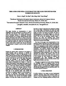
1. Introduction Stony corals exist in many shapes and sizes. The shape of a coral is not only determined by genetics, but also by environmental factors, such as the amount of available light, water flow speed, and availability of food, [Kaa99]. Thus, within a single species the shape can show a high degree of variation. Understanding of the external factors influencing the growth and shape of coral colonies is essential in clarifying their role in marine ecosystems, and to explain their susceptibility to pollution and global climate change, [KSM∗ 05]. Currently, coral biologists analyze coral shape by performing manual measurements on photographs of coral colonies. This is a laborious, error prone and subjective task. Although it may suffice for simple colonies, it is not adequate for the analysis of complex three-dimensional branching coral structures, such as the coral shown in the left image of figure 1. We propose to simplify the measuring procedure with interactive visualization. The approach is depicted in figure 1. Given a Computer Tomography (CT) scan of a coral, a skeleton of the coral is extracted, measurements of various morphological properties are performed on the skeleton graph, and statistical distributions of the measurements are generc The Eurographics Association 2006.
ated. By analyzing these distributions, coral biologists can classify and compare corals in a robust and quantitative way. In this paper we describe an interactive visualization system for measuring branching coral shapes. Instead of discussing the details of all steps in the system, we focus on areas which greatly influence the visualization methods. Ideally, such a system should be fully automated. Unfortunately, due to many reasons automation cannot be realized, and we will report in which steps interaction is required. 2. Related Work While the application area of our work is novel, similar systems have been developed for the analysis of a variety of medical data, using various techniques. Martínez-Pérez et. al. [MPHS∗ 00] have quantified blood vessel morphology in 2D retinal images, using skeletons. Measureable differences have been found between healthy and diseased venous systems. The metrics included lengths, areas and bifurcation angles. More commonly, analysis of medical data is focused on measuring single items, such as vessel diameter along single
K. J. Kruszy´nski, R. van Liere & J. A. Kaandorp / An Interactive Visualization System for Quantifying Coral Structures 0.16 0.14 0.12 0.10 0.08 0.06 0.04 0.02 0.00
394 simp spacing 0 full
0
5
10
15
20
mean: 6.3444, stddev: 2.5676 min: 0.4548, max: 12.1895, #: 173
25
Figure 1: The approach used by the system, using a skeleton to quantify the morphology of the scanned coral.
vessel path, [BRL∗ 04]. In another system, [PTSP02], interaction is used to measure relevant objects or distances directly in volume data, while it is also possible to use Principal Component Analysis (PCA) to automatically determine the extent of an object, or the angle between two objects. The hierarchy of vessel systems can also be used to provide advanced visualizations of complex structures, for use in surgery planning [HPSP01].
lead to erroneous measurement results, and thus lead the scientist to wrong conclusions about the coral.
The main focus of medical systems is on interactive data exploration, instead of comprehensive morphological analysis, and visualizations are used to gain insight about the data, not only to aid processing.
Figure 2: System overview.
3. System Requirements One approach to quantify the morphology of complexshaped branching objects like corals is by using measurements based on the medial axis (or morphological skeleton, [Blu67]) of the object. It is essential that this skeleton is a correct representation of the topology and geometry of the coral. This depends to a high degree on the choice of a suitable skeletonization algorithm [KvLK05]. In addition, an optimal skeletonization and accurate measurement depends on the quality of the segmentation of the object. Due to various difficulties with coral, artifacts in the data set, and the specifics of the various techniques and algorithms, additional processing is necessary. Some of this processing cannot be carried out automatically, but must be performed manually. In such cases, the system must assist the person performing the processing task. For other processing tasks, the results depend on a proper choice of one or more parameters, and the system must facilitate the assessment of different parameter choices. In any case, it should be possible to check the results of each step, whether automatic or manual, to confirm the proper operation of the system. Visual comparison with the actual colony can indicate whether an operation has introduced any undesired artifacts into the data set. The amount of modifications applied to the data should also be minimized, since any operation performed on the data can introduce artifacts into the data. These can in turn
4. System Overview Coral
Scanning
Filtering
Segmentation
Skeleton Extraction
Skeleton Graph Processing
Measuring
Statistical Analysis
An overview of the steps performed by the system is shown in figure 2. A coral colony is scanned at a high resolution using a CT scanner, which results in a 3D volumetric data set. Noise in the data is filtered using a smoothing filter, and the filtered data is visually inspected to determine the optimum amount of filtering. The data is then segmented using a region growing technique. One or more seed points are interactively marked in the data, and the correctness of the segmentation is assessed by visual comparison of the visualized segmentation both with the scan, and with the actual coral colony. Holes and cavities in the segmented data are automatically located and filled, after which a manual check of the filled areas is performed. From the segmented volume a morphological skeleton is extracted, which is then converted to a graph representation [RJP00]. The next step is the removal of loops from the skeleton. The loops are automatically highlighted, but the cut location must be selected manually. If deemed necessary, additional branches or whole sections of the skeleton can be removed manually, or by length thresholding. It is also possible to straighten the lines of the skeleton by a selectable amount. To enable correct measurements, the root of the coral is selected manually, and the proper orientation of the coral with respect to the ground is established interactively. The branches of the skeleton are then ordered using a HortonStrahler ordering [YM94], in order to split the measurement results by branch order. The distance transform [Bor86] of the segmented volume, needed to measure the thickness of the coral, is calculated, or loaded from disk. c The Eurographics Association 2006.
K. J. Kruszy´nski, R. van Liere & J. A. Kaandorp / An Interactive Visualization System for Quantifying Coral Structures
5.1. Noise CT scans of corals tend to contain noise artifacts in the center part of the coral. This is presumably a result of the scattering of X-rays by the coral.
(a) Minimum and maximum thickness.
(b) Branching angles.
Corals also tend to have an uneven surface, because part of the surface might have eroded away as a result of longterm exposure to the marine environment. Furthermore the surface might be partly covered by encrusting animals or algae, and the colony might be damaged by boring organisms, such as for example sponges or certain worms. All these artifacts may show up on the CT scan. If such artifacts are small, they can be filtered from the scan using some type of image smoothing filter. Because simple filters also tend to change the shape and location of object edges in the image, which are important to the measuring process, we have chosen to use a rather advanced filter, which leaves larger edges mostly intact.
(c) Geotropy angles.
(d) Branch spacing.
Figure 3: Examples of the measurement method of five different morphological properties.
After this, the morphological properties of the coral can be measured, using several measurements specific to the morphology of branching corals and similar organisms [KL04]; figure 3 shows how five of these measurements are obtained. Figure 3(a) shows the minimum and maximum branch thickness; this is measured with spheres located at branching points (maximum thickness, white disc), and spheres located directly adjacent to these (minimum thickness, black disc). Figure 3(b) shows the branching angles, figure 3(c) shows the geotropy angles, and figure 3(d) shows the branch spacing. The raw measurement data is compiled into histograms for easy analysis. The mean, standard deviation, and other statistics are also calculated. Both cumulative and per-order statistics are provided. Measurements from different specimens are subjected to a non-parametric rank test, to quantify the similarities or differences between specimens. 5. Problems and Solutions As stated earlier, conceptually the system is very simple. The input dataset is filtered, segmented, and a skeleton is extracted. This skeleton is then measured, and the measurements are then analyzed and displayed in some convenient form. However, on a detailed level there are many difficulties to be overcome. Some are handled by automatic processing, and some require manual intervention. c The Eurographics Association 2006.
A close-up volume rendering of a part of a coral colony, with various amounts of noise reduction filtering applied, is shown in figure 4. The filter is very successful in removing noise, but it is advisable to limit the number of iterations of the filter, because too much filtering can cause disjoint but closely adjacent branches to fuse together. Although such artificial branch fusion can be detected automatically, the unnecessary introduction of such artifacts into the data should be avoided. Visual comparison of the filtered scan with the original colony can be used to determine the optimal amount of filtering.
(a) Original
(b) Four iterations
(c) Eight iterations
Figure 4: Close-up volume rendering after various amounts of noise reduction.
5.2. Damage Coral colonies are very fragile objects, and the branches break off easily. Because a coral colony must be transported from the original growth site, or from a museum collection, to some location equipped with a CT scanner, it is almost impossible to avoid all damage. Broken branches are often reattached to the rest of the colony using some type of glue. Because glue has a lower density than the original coral, the CT scan contains a lower density gap between the two parts. For the purpose of studying the shape of the coral, the low density gap should be
K. J. Kruszy´nski, R. van Liere & J. A. Kaandorp / An Interactive Visualization System for Quantifying Coral Structures
Figure 5: Cross-section showing a clear fracture.
treated as being part of the coral. A cross-section of such a broken and reattached branch is shown in figure 5. Finding a suitable starting point for the segmentation is often a matter of trial and error, and even a seemingly correct segmentation should be carefully inspected, to determine whether glued branches have also been included in the segmentation. A visualization of the segmented coral can be compared with the filtered scan, to visually determine if the segmentation has included parts of the volume which do not belong to the coral, or if it has left out parts which do belong to the coral. The original colony must also sometimes be used for this purpose, since it is not always possible to determine the nature of some artifacts using only the scan. It can also be decided to ignore certain parts of the coral for the purpose of the analysis, or to study only one part of the colony. For example, the colony may have suffered extensive damage, or a part of it may have died and slowly decayed a long time before the study. The system provides an easy method of selecting a part of the skeleton, and either removing it, or keeping only the selected part. 5.3. Holes Coral has a high density near its surface, but a very low density in the center. The result is that in CT scans, there is not a very large difference between the inside of the coral and the background. Especially in the center of the coral, where there is noise in the scan as a result of the scanner ray being scattered, the difference between the inside of the coral and the background cannot be readily determined, as the density values are hardly distinguishable. Thus segmenting a CT scan of a coral will result in cavities inside the object. If the dense outer layer is very thin in some location, or even absent, for example due to a drilled hole, the result is that the cavity inside the segmented object is actually connected to the background. This kind of cavity is called a hole, and an example can be seen in figure 6. Cavities and holes in the segmented coral make proper skeletonization and measurement very difficult and unreliable, due to their effects on skeletonization algorithms and
Figure 6: Part of a slice from a scanned coral, clearly showing a hole.
distance transforms, so they must be filled up. While it is trivial to fill a cavity which is completely enclosed inside the object, filling holes connected to the outside presents quite a challenge. A cavity in an object is defined as a set of connected background voxels, which is surrounded by object voxels. These background voxels thus form a ‘bubble’ inside the object. These cavities can easily be found by using an appropriate flood-fill algorithm. If the background of the volume is filled with the same value as the object, then the only remaining background voxels are those that belong to the cavities. Thus, if it is known that an object is not supposed to have any cavities, these can easily be found and filled. Holes are cavities which have a connection to the regular background in the volume. Due to this connection, it is not possible to locate them using a flood-fill algorithm, as there is no boundary between the hole and the background. However, if the volume is divided into 2D slices, it can be seen that in many of these slices the part corresponding to the hole is actually an island of background values fully enclosed by foreground values, as would be the case with a cavity. By combining this information from many slices, cut in different directions from the volume, it is possible to locate most of the voxels belonging to the hole. In our system, first all cavities are filled with a regular flood-fill. Then the remaining holes are filled by considering the volume slice-by-slice, with slices perpendicular to the primary axes, as well as slices perpendicular to the side diagonals of the volume. The background in each slice is flood-filled with the foreground value, and then inverted, so the only remaining foreground voxels in the slice are those belonging to a hole. These slices are then recombined into a new volume using a logical OR operation. The whole process is performed a second time on the output of the first run, to fill some remaining gaps which could not be filled in the first iteration. c The Eurographics Association 2006.
K. J. Kruszy´nski, R. van Liere & J. A. Kaandorp / An Interactive Visualization System for Quantifying Coral Structures
Since it is possible that this method would fill up areas which would not be considered holes, the fillings must be checked manually by the user. This is done by showing the user each filling, along with the original object. The user can then decide for each filling whether it is correct or not, and only the correct ones are then combined with the object. Because most of the fillings created by this method are very small, and not likely to be very significant, they are ordered by decreasing size. The user can then decide that any filling smaller than the current one will be insignificant, even if incorrect, and stop checking more fillings.
skeleton. This is shown in figure 8. A potential pitfall here is that branches which have very recently formed, and are thus still very short, will also be removed from the data, and will not be measured.
5.4. Skeleton Loops Some of the used measurements require the skeleton branches to be ordered. This hierarchical ordering of branches is only possible if the skeleton contains no loops, but unfortunately this is usually not the case. Loops can appear in coral skeletons either as an artifact of insufficient scanner resolution, or because the branches of the coral have actually grown back together.
Figure 8: Removing short end branches from the skeleton.
5.6. Discretization Artifacts Because the skeleton is voxel-based, it will contain aliasing artifacts. These appear in the form of jagged lines, which should have been straight. If this is considered to be a problem, for example because it increases the length of a branch, the lines can be straightened out [RJP00]. The parameter for this simplification can be interactively selected; a proposed new skeleton, with a very large amount of simplification, is shown highlighted in figure 9.
Figure 7: Skeleton with loops highlighted. To properly perform the measurements, these loops must be disconnected. To our knowledge there is currently no algorithm available which can detect the exact location of fusion points of branches, or determine how much of the skeleton should actually be removed. Due to this lack of automatic methods, user interaction is required for this task. The system can only assist by highlighting the loops in the skeleton, as shown in figure 7.
Figure 9: Simplification of the skeleton.
5.5. Skeleton Noise
6. Implementation
As a result of the unevenness of the surface of the coral, even after filtering, the skeleton may contain many ’false branches’. These are branches which do not correspond to an actual branch of the coral, but rather to a small disturbance on the surface. While these branches could be removed manually from the skeleton, there can be a lot of such branches, and it is easier to remove them by defining a minimum length for such branches. All end branches which are shorter than the threshold value are then removed from the
The filtering and segmentation has been implemented using standard filters from the Insight Segmentation and Registration Toolkit (ITK). The filtering is done using the ITK Curvature Flow filter, while the segmentation utilizes the ITK Confidence Connected filter. The Visualization Toolkit (VTK) is used to show the results of the filtering and segmentation, and to interactively select the segmentation starting point. The visualization techniques used include 3D volume rendering, translucent and solid 3D iso-surfaces, 2D
c The Eurographics Association 2006.
K. J. Kruszy´nski, R. van Liere & J. A. Kaandorp / An Interactive Visualization System for Quantifying Coral Structures
slice images, and 3D geometric representations of the skeletal graph and some measurement results. Unfortunately, there is no filter in either the Insight Toolkit or the Visualization Toolkit which can fill holes in binary volumes. Also, most work in the area of hole filling is focused on either patching clearly defined gaps in mesh surfaces [DMGL02], or retouching gaps in 2D images [BSCB00]. We have therefore devised and implemented our own crude filling algorithm for 3D volumes, using an existing VTK filter as the basis. This algorithm was described in section 5.3. As stated before, the output of this algorithm requires interactive inspection. A skeletonization algorithm proposed by W. Xie [XTP03] has also been implemented as a VTK filter. Although there are no 3D volume skeletonization filters in either ITK or VTK, the main reason for an own implementation was that the choice of the specific algorithm had already been made before [KvLK05]. After skeletonization, the voxel-based skeleton is converted into a graph representation, using VTK geometry data structures, with lines connecting neighboring voxels. All the remaining parts of the system operate on these lines. As VTK lacks a filter to perform either the conversion to lines, or many of the other tasks required for the system, this too has made the development of several new VTK filters necessary. 6.1. Performance Due to the size of the CT scans (typically 512 × 512 × 512 voxels, 512 MB of data if single-precision floating point is used), the performance of the system during some steps is very dependent on the amount of available memory. The filtering is a particularly memory-intensive operation, as it not only uses floating-point values for all voxels, but also keeps several copies of the data in memory at the same time. On our test system, equipped with an AMD Athlon64 3800+ CPU and 2 GB of memory, the filtering takes approximately 80 seconds per iteration of the algorithm, depending on the size of the volume, assuming that a typical volume has a size of 5123 voxels. The amount of time needed for segmentation, assuming a suitable starting point is chosen, depends mainly on the volume occupied by the object being segmented. We have observed times between 20 seconds and 2 minutes. If an incorrect starting point is chosen, it is possible that either the background, or the whole volume is marked as the object of interest. In that case, the segmentation takes more time to complete than the time required with a correct starting point. The hole filling algorithm requires the most time to complete. The time to perform the two filling iterations used by the system ranged from 7 to 11 minutes for the data analyzed in section 7. It also takes several minutes to manually check the results.
For the same data, we have observed the skeletonization algorithm to take from 30 seconds to 2 minutes to complete. This time depends on the volume occupied by the object, and on the thickness of the object. A thin object will require less iterations to extract the skeleton than a thick object occupying the same number of voxels. The calculation of the distance map, which is needed for the measurements, requires a great amount of memory for large volumes. The time to calculate the distance maps for the previously mentioned data ranged from 80 seconds up to nearly 4 minutes, with the latter being partly due to the process using more than the available 2 gigabytes of RAM, with some amount of disk swapping slowing the process down. Once the distance map is either calculated or loaded from disk, the actual measuring and the generation of the histograms takes no longer than 30 seconds. Typical total times required for processing an average data set range from 30 to 45 minutes. 7. Results We have used the system to compare three specimens of the scleractinian coral species Madracis mirabilis, which is native to the Caribbean region. The three coral colonies were scanned at a resolution of 0.25 mm×0.25 mm×0.3 mm, with a slice size of 512 × 512 pixels. The specimens were named object 389, object 393 and object 394. The respective number of slices in each scan is 541, 373 and 329. A volume rendering of these three specimens is shown on the far left in figure 10. Note that these renderings are not on the same scale. It can easily be seen that objects 393 and 394 differ significantly in their compactness, and it is assumed that object 389 constitutes an intermediate form between these two. All three specimens have been denoised using four iterations of the denoising filter, as this was determined to be the optimal setting for this particular data. The close-up of a part of object 394 in figure 4 demonstrates the effect of the filtering. 7.1. Visual Results The results of segmentation of the three objects are shown in the second column from the left in figure 10. Visual comparison with the original object, and with the scan, indicates that the segmentation is correct. The corresponding morphological skeleton of each specimen can be seen in the third column of figure 10. The loops have already been removed from these skeletons, and some simplification has been applied. 7.2. Quantitative Results Because the system produced a large amount of data (225 histograms were generated), and a detailed discussion of all c The Eurographics Association 2006.
K. J. Kruszy´nski, R. van Liere & J. A. Kaandorp / An Interactive Visualization System for Quantifying Coral Structures
393 simp length
0.25
0.15
0.15
0.10
0.10
0.05
0.05 0.00
0
10
20
30
40
50
mean: 13.0587, stddev: 7.2246 min: 1.3238, max: 36.1210, #: 131
389 simp length
0.25
40
60
80
100 120 140 160
mean: 91.0182, stddev: 13.5565 min: 65.0784, max: 126.6317, #: 65
389 simp branching angles
0.15
0.15
0.10
0.10
0.05
0.05 0
10
20
30
40
50
mean: 11.9531, stddev: 7.8975 min: 0.2500, max: 45.0887, #: 351
394 simp length
0.25
0.00 20
40
60
80
100 120 140 160
mean: 86.1671, stddev: 16.8633 min: 35.7458, max: 133.2493, #: 175
0.20
0.20
394 simp branching angles
0.15
0.15
0.10
0.10
0.05
0.05 0.00
0.00 20
0.20
0.20
0.00
393 simp branching angles
0.20
0.20
0
10
20
30
40
50
mean: 8.2097, stddev: 5.6853 min: 0.2500, max: 33.4369, #: 345
0.00 20
40
60
80
100 120 140 160
mean: 90.8736, stddev: 21.9380 min: 30.0959, max: 144.9805, #: 172
Figure 10: From top to bottom: object 393, object 389, and object 394. From left to right: Volume rendering of the CT scan, iso-surface of the segmentation, the skeleton, a histogram of the branch lengths, and a histogram of the branching angles thickness.
results is beyond the scope of this paper, we shall only highlight two of the obtained results. The histograms in figure 10 show the values of the measurements on the X-axis, and the frequency distribution of these values on the Y-axis. From top to bottom, each set of histograms shows the distribution for object 393, 389 and 394. This order is used because object 389 is believed to be an intermediate form between object 393 and object 394. The left histograms in figure 10 show the lengths of the branches of each coral. This metric is defined as the distance along the skeleton between succesive branching points. The graph shows that the branches of object 393 are on average slightly longer than the branches of object 389, while the branches of object 394 are significantly shorter. Thus in the case of branch length, object 389 might be considered an intermediate form. The right histograms in figure 10 show the branching angles. These are the angles between branches originating at a common branching point, as illustrated in figure 3(b). The histograms show that the average angle is very similar for all three objects, but the deviation from this average is the smallest for object 393, and the largest for object 394, with object 389 again in the middle. c The Eurographics Association 2006.
8. Conclusion In this paper we describe a procedure for the morphological quantification of branching complex-shaped objects. This procedure can be applied to a broad class of biotic and abiotic branching objects. In coral taxonomy [VP76] the morphological description of coral colonies is usually highly qualitative. In our approach we are able to make a true quantitative differentiation between morphologies of different coral species. Furthermore the method can be used to investigate the impact of the physical environment on the morphology. In simulation studies on growth and form of coral colonies [KSM∗ 05], the availability of methods for comparing simulated and actual growth forms is a crucial prerequisite. We have described the various problems which can occur when attempting to quantify coral morphology. There can be noise in the data, the coral colony can have sustained damage, and the structure of the coral itself makes it difficult to perform a proper segmentation. The morphological skeleton can contain loops, which must be disconnected, and various other artifacts. All these issues have an influence on the quantification of the morphology of the coral, and must be properly resolved in order to perform an accurate quantitative analysis. Interactive visualization is an essential part of the quan-
K. J. Kruszy´nski, R. van Liere & J. A. Kaandorp / An Interactive Visualization System for Quantifying Coral Structures
tification process. It is necessary, because some tasks cannot be performed automatically, such as disconnecting any loops present in the skeleton. Sometimes it is also needed in order to correct the results of automatic processing, or to provide the quantification system with information which it cannot infer from the data. Finally, it is used to verify that the system does not introduce artifacts into the data, and thus to make sure that the obtained results are indeed accurate and reliable. Acknowledgments This work was carried out in the context of the Virtual Laboratory for e-Science project (www.vl-e.nl). This project is supported by a BSIK grant from the Dutch Ministry of Education, Culture and Science (OC&W) and is part of the ICT innovation program of the Ministry of Economic Affairs (EZ). We thank G.J. Streekstra and H. Venema for their help and advice in obtaining CT-scans of the corals. References [Blu67] B LUM H.: A transformation for extracting new descriptors of shape. In Models for the Perception of Speech and Visual Forms, Wathen-Dunn W., (Ed.). MIT Press, Amsterdam, 1967, pp. 362–380. [Bor86] B ORGEFORS G.: Distance transformations in digital images. Computer Vision, Graphics, and Image Processing 34 (1986), 344–371. [BRL∗ 04]
B OSKAMP T., R INCK D., L INK F., K UM MERLEN B., S TAMM G., M ILDENBERGER P.: New Vessel Analysis Tool for Morphometric Quantification and Visualization of Vessels in CT and MR Imaging Data Sets. Radiographics 24, 1 (2004), 287–297.
[BSCB00] B ERTALMIO M., S APIRO G., C ASELLES V., BALLESTER C.: Image inpainting. In Siggraph 2000, Computer Graphics Proceedings (2000), Akeley K., (Ed.), ACM Press / ACM SIGGRAPH / Addison Wesley Longman, pp. 417–424. [DMGL02] DAVIS J., M ARSCHNER S. R., G ARR M., L EVOY M.: Filling holes in complex surfaces using volumetric diffusion. In Proceedings First International Symposium on 3D Data Processing Visualization and Transmission (3DPVT’02) (2002), pp. 428–439. [HPSP01] H AHN H. K., P REIM B., S ELLE D., P EITGEN H. O.: Visualization and interaction techniques for the exploration of vascular structures. In VIS ’01: Proceedings of the conference on Visualization ’01 (Washington, DC, USA, 2001), IEEE Computer Society, pp. 395–402.
[KL04] K AANDORP J., L EIVA R. G.: Morphological analysis of two- and three-dimensional images of branching sponges and corals. In Morphometrics and their applications in Paleontology and Biology (Berlin, 2004), Elewa A., (Ed.), Springer-Verlag, pp. 83–94. [KSM∗ 05] K AANDORP J., S LOOT P., M ERKS R., BAK R., V ERMEIJ M., M AIER C.: Morphogenesis of the branching reef coral madracis mirabilis. Proc. Roy. Soc. Lond. B 272 (2005), 127–133. ´ [KvLK05] K RUSZY NSKI K. J., VAN L IERE R., K AAN DORP J.: Quantifying differences in skeletonization algorithms: A case study. In Visualization, Imaging, and Image Processing (VIIP 2005), Benidorm, Spain, September 7-9 (September 2005), Villanueva J. J., (Ed.), IASTED, ACTA Press, pp. 666–673.
[MPHS∗ 00] M ARTÍNEZ -P ÉREZ M. E., H UGHES A. D., S TANTON A. V., T HOM S. A., C HAPMAN N., B HARATH A. A., PARKER K. H.: Geometrical and morphological analysis of vascular branches from fundus retinal images. In MICCAI ’00: Proceedings of the Third International Conference on Medical Image Computing and Computer-Assisted Intervention (London, UK, 2000), Springer-Verlag, pp. 756–765. [PTSP02] P REIM B., T IETJEN C., S PINDLER W., P EITGEN H. O.: Integration of measurement tools in medical 3d visualizations. In VIS ’02: Proceedings of the conference on Visualization ’02 (Washington, DC, USA, 2002), IEEE Computer Society, pp. 21–28. [RJP00] R EINDERS F., JACOBSON M. E. D., P OST F. H.: Skeleton graph generation for feature shape description. In Data Visualization 2000 (2000), Leeuw W. d., Liere R. v., (Eds.), Springer Verlag, pp. 73–82. [VP76] V ERON J., P ICHON M.: Scleractinia of eastern Australia part I: Families Thamnasteriidae, Astrocoeniidae, Pocilloporidae. Australian Government Publishing Service, Canberra, 1976. [XTP03] X IE W., T HOMPSON R. P., P ERUCCHIO R.: A topology-preserving parallel 3D thinning algorithm for extracting the curve skeleton. Pattern Recognition 36 (July 2003), 1529–1544. [YM94] Y EKUTIELI I., M ANDELBROT B. B.: Hortonstrahler ordering of random binary trees. Journal of Physics A: Mathematical and General 27, 2 (1994), 285– 293.
[Kaa99] K AANDORP J.: Morphological analysis of growth forms of branching marine sessile organisms along environmental gradients. Mar. Biol. 134 (1999), 295–306. c The Eurographics Association 2006.