An Introductory Tutorial on Stochastic Linear. Programming Models. Suvrajeet
Sen. Department of Systems and Industrial Engineering. The University of
Arizona.
An Introductory Tutorial on Stochastic Linear Programming Models Suvrajeet Sen
Department of Systems and Industrial Engineering The University of Arizona Tucson, Arizona 85721
Julia L. Higle
Department of Systems and Industrial Engineering The University of Arizona
Linear programming is a fundamental planning tool. It is often difficult to precisely estimate or forecast certain critical data elements of the linear program. In such cases, it is necessary to address the impact of uncertainty during the planning process. We discuss a variety of LP-based models that can be used for planning under uncertainty. In all cases, we begin with a deterministic LP model and show how it can be adapted to include the impact of uncertainty. We present models that range from simple recourse policies to more general two-stage and multistage SLP formulations. We also include a discussion of probabilistic constraints. We illustrate the various models using examples taken from the literature. The examples involve models developed for airline yield management, telecommunications, flood control, and production planning.
O
ver the past several decades, linear programming (LP) has become a fundamental planning tool. It is routinely applied in engineering, business, economics, environmental studies, and other disciplines. This widespread acceptance may be due to (1) good algorithms, (2) practi-
tioners’ understanding of the power and scope of LP, and (3) widely available and reliable software. Furthermore, research on specialized problems, such as assignment, transportation, and network problems, has made LP methodology indispensable in many industries, including
Copyright q 1999, Institute for Operations Research and the Management Sciences 0092-2102/99/2902–0033/$5.00 This paper was refereed.
PROGRAMMING, STOCHASTIC TUTORIAL
INTERFACES 29: 2 March–April 1999 (pp. 33–61)
SEN, HIGLE airlines, energy, manufacturing, and telecommunications. Notwithstanding its successes, however, the assumption that all model parameters are known with certainty limits its usefulness in planning under uncertainty. When one or more of the data elements in a linear program is represented by a random variable, a stochastic linear program (SLP) results. In deterministic activity analysis, planning consists of choosing activity levels that satisfy resource constraints while maximizing total profit (or minimizing total cost). All the information necessary for decision making is assumed to be available at the time of planning. Under uncertainty, not all the information is available, and some parameters should be modeled as random variables. We discuss here models that can include random variables within optimization problems. Since deterministic methodology has been prevalent in optimization models, it may be tempting to suggest that random variables should be replaced by their means and the resulting optimization problem solved. In general, this approach provides solutions that are structurally different from those provided by stochastic optimization models. To understand this, consider a network with n nodes, as in Figure 1, on which demand for connections between the (n2 ) demand pairs must be accommodated. Networks, such as those in telecommunications systems, are complex and typically include hundreds of nodes. In the design problem that we consider, the capacity of each network link must be determined in anticipation of future demand requirements. It is customary to assume that the
requirements between various node pairs are known with certainty. Such deterministic network-design problems result in a tree structure (Figure 2a). With a tree design, all demand pairs have paths through which calls may be routed. However, the design is rigid in that only one such path is available. During periods of high demand, the lack of alternative routes results in the rejection of calls and a reduced level of service. Moreover, if a link should fail because of some catastrophic event, nodes will be disconnected from the network. Attempts to counter these difficulties by scaling the demand upward, for example, will increase the capacity of the links used; it will not eliminate the rigidity of the design. To obtain a more flexibly designed network (Figure 2b), one must incorporate the need for flexibility within the model. One must construct a model that explicitly considers the likelihood of periodic (and correlated) heavy loads on segments of the network and the possibility of catastrophic equipment failures. The improvement possible from the use of a stochastic model increases with the size of the network. In fact, in a case study conducted at Bellcore, Sen, Doverspike, and Cosares [1994] report a 75-percent reduction in the number of lost calls using stochastic LP models in place of deterministic models. Methods for forecasting important quantities, such as demand, are well known and widely used. Moreover, the fields of statistics and simulation provide methods for obtaining distributional representations of these quantities when point estimators are inadequate. Although many people routinely formulate LP models, only recently have OR/MS practitioners
INTERFACES 29:2
34
STOCHASTIC LINEAR PROGRAMMING
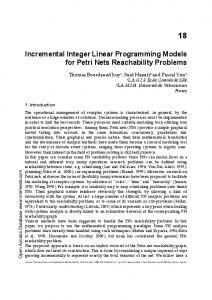
Figure 1: In this simple network with three nodes, there are (32), or three point-to-point demand pairs: A-B, B-C, and A-C. The presence of an edge indicates that capacity may be added to form a link between the two nodes in the network.
begun using these methods to formulate LP models for decision making under un-
certainty. In this tutorial, we explain linear-programming models for optimization under uncertainty at a very elementary level. Consequently, all we assume is that readers are familiar with LP models and elementary probability constructs. The Impact of Uncertainty The presence of uncertainty affects both feasibility and optimality. In fact, formulating an appropriate objective function itself raises interesting modeling and algorithmic questions. Feasibility Under Uncertainty To incorporate uncertainty within an LP, one must define feasibility. Two naive approaches have sometimes been adopted in practice. Example 1: SLPs with Expected Values Consider the following four variable deterministic LP: Minimize 1x2 subject to x1 ` x2 ` x3 4 2 1x1 ` x2 ` x4 4 2 11 # x1 # 1 xj > 0, j 4 2, 3, 4.
(1)
Suppose that the coefficients of x1 and x2 in (1) are not known with certainty, and all that is known about these parameters is their joint distribution (a˜21, a˜22)
5
11, 342 with probability 12 113, 542 with probability 12 .
Figure 2: These illustrate alternative network designs. The tree structure in 2a results from the use of a deterministic model and yields a very rigid routing protocol. The network in 2b results from the use of a stochastic model. It is a more flexible design due to the presence of multiple routing capabilities for each demand pair. In general, the design in 2b provides a greater opportunity to respond to network failures and high loads than the design in 2a.
In this case, E[a˜21] 4 11 and E[a˜22] 4 1 so that the coefficients in (1) correspond to the expected values of the random variables. In examining this formulation, we first investigate whether its solution, (x1,
March–April 1999
35
4
SEN, HIGLE x2, x3, x4) 4 (0, 2, 0, 0)), is feasible under uncertainty. Under uncertainty, the constraint corresponding to (1) is equally likely to be either
The vector (0, 2, 0, 0) does not satisfy either of these equations and thus is infeasible under uncertainty! Under uncertainty, the formulation in which random variables are replaced by their expected values may not provide a solution that is feasible with respect to the random variables. Example 2: Wait and See Another approach that practitioners often adopt is based on a wait-and-see analysis (sometimes referred to as scenario analysis or what-if analysis). This approach mimics the process of delaying all decisions until the last possible moment, after all uncertainties have been resolved. As a result, the LPs associated with all possible outcomes of the random quantities are solved. This yields a collection of decision vectors, one for each possible outcome of the random variable(s). In general, none of these solutions may be worthwhile. For example, consider the two possible realizations of the problem in Example 1. The solution associated with (a˜21, a˜22) 4 (1, 3/4) is (11, 3, 0, 0.75), while the solution associated with (a˜21, a˜22) 4 (13, 5/4) is (12/17, 32/17, 0, 0.75). As with the solution to the expected-value problem, neither of these solutions is feasible with respect to the alternate outcome.
That is, if implemented, either solution would have a 50-percent chance of failing to satisfy a constraint. As illustrated by Examples 1 and 2, an appropriate decision-making framework under uncertainty should explicitly consider the consequences of future infeasibility within the model. This aspect of modeling responses to future infeasibility sets stochastic programs apart from their deterministic counterparts. In the stochasticprogramming literature, two approaches are widely studied: one is based on modeling future recourse (response) and another restricts the probability of infeasibility (typically equivalent to system failures) to be no greater than a prespecified threshold. The first approach yields the so-called recourse problems, and the second approach yields problems with probabilistic (or chance) constraints. While a specific application may call for both approaches, we discuss them separately. The stochastic-programming literature also considers another problem: the distribution problem. Researchers focus on characterizing the distribution of the optimal value or optimal solutions of random LPs. As with wait-and-see problems, the distribution problem does not provide a decision-making framework. Nevertheless, it provides a mathematical common ground between the second-stage random LP in recourse problems and the random LP of the wait-and-see approach. From a computational point of view, this problem remains a major challenge [Pre´kopa 1995, chapter 15]. Objectives Under Uncertainty A great deal of research revolves around the choice of objectives in decision
INTERFACES 29:2
36
x1 `
3 x2 ` x4 4 2 4
or 13x1 `
5 x2 ` x4 4 2. 4
STOCHASTIC LINEAR PROGRAMMING making under uncertainty. One of the more common objectives is to optimize expected costs (or returns). However, as decision makers, we might be interested in the variability of costs (or returns) associated with a plan. More generally, a decision maker’s choices may be guided by a utility function. In decision-making models for an individual, the concept of a utility function has many merits, although its specification can be elusive. The notion of a utility function can become even more elusive in large-scale applications of LP. In the following, we discuss four of the more common objectives for large-scale LPs under uncertainty: (1) Minimization of expected costs is by far the most common objective used in large-scale optimization under uncertainty. For such applications as planning power generation, average seasonal cost per day reflects the repetitive cost of supplying electricity. For some applications in telecommunications systems, system performance is often measured in terms of average unserved demand. Finally, in production-and-inventory systems, it is common to use average production and holding costs in evaluating the cost effectiveness of a system. For such systems, the expected cost criterion is easily justified. (2) Minimization of expected absolute deviations from goals is a class of objectives that results from extending goalprogramming techniques to account for uncertainty. In some cases, it may be advantageous to specify goals that depend upon particular scenarios. For example, production goals may depend upon economic factors that are modeled as uncertain quantities. Thus, the goals associated
with prosperous and recessionary times may be decidedly different. To meet such managerial objectives under uncertainty, it may be appropriate to minimize expected absolute deviations from set goals. (3) Vector optimization under uncertainty is a class of models that generalize the stochastic goal-programming approach. An example of a multiobjective model would be a traveler’s advisory system to recommend routes from origin to destination in Tucson, Arizona. Because flash floods occur during the monsoon season in Tucson, the advisory system must include low water level on the roads as one of the objectives. In addition, it should incorporate the traditional objective of minimal travel time. Because these objectives are essentially noncommensurate, it is appropriate to adopt the vector-optimization framework. Furthermore, since the route is to be recommended before a potential downpour, water levels are random variables (as are travel times). This results in a vector-optimization problem under uncertainty. (4) Minimization of maximum costs is an alternate class of models. There are various interpretations of the term minimax in stochastic-programming models. In one interpretation, no distributional information is available, and all that is known is the set of possible outcomes. In this case, the minimax objective minimizes the maximum loss among all possible outcomes of the random variable. A similar class of problems arises in the case of partial information regarding the probability distributions. For instance, one may have information regarding some characteristics of the distribution (for example, support, mean,
March–April 1999
37
SEN, HIGLE and variance), and the set of probability measures of interest may be those that share those characteristics. A worst-case approach under partial information is one in which we choose a decision that minimizes maximum expected loss, regardless of the distribution (from among the class with the specified characteristics). When the class of distributions can be characterized as a polyhedral set, this class of problems can be solved using generalized LP. This minimax approach is known to be conservative and may be appropriate in models that plan to avoid catastrophes. Thus, models associated with environmental planning may appropriately use this objective [Pinter 1991]. In this tutorial, we discuss primarily models with the expected value objective. Two-Stage Recourse Models In two-stage recourse models, we explicitly classify the decision variables according to whether they are implemented before or after an outcome of the random variable is observed. Decisions that are implemented before are known as first-stage decisions while those after are second-stage decisions. The first-stage decision variables can be regarded as proactive and are often associated with planning issues, such as capacity expansion or aggregate production planning. Second-stage decision variables can be regarded as reactive and are often associated with operating decisions. These second-stage decisions allow us to model a response to the observed outcome, which constitutes our recourse. When outcomes are revealed sequentially, decision making involves a multistage planning problem. In recourse planning, we model a re-
sponse for each outcome of the random elements that might be observed. In general, this response will also depend upon the first-stage decisions. In practice, this type of planning involves setting up policies that will help the organization adapt to the revealed outcome. For example, in production and inventory systems, the first-stage decision might correspond to production quantities, and demand might be modeled using random variables. When demand exceeds the amount produced, policy may dictate that customer demand be backlogged at some cost. This policy constitutes a recourse response. The exact level of this response (the amount backlogged) depends on the amounts produced and demanded. Under uncertainty, it is essential to adopt initial policies that will accommodate alternative outcomes. Consequently, modeling under uncertainty requires that we incorporate a model of the recourse policy. In some applications, it is possible to deviate from prescribed limits, although with a penalty cost. For example, in production and inventory management, a backlogging policy leads to shortage costs whenever the demand exceeds the amount in stock. Such a policy is called a simple recourse policy, which we illustrate using the data from Example 1. Example 3: A Simple Recourse Model Consider the data for Example 1 and suppose that the variables (x1, x2, x3, x4) are all first-stage (planning) variables. Suppose that the recourse policy allows one to compensate for second-stage discrepancies by incurring a penalty cost of 5 per unit of deviation from the right-handside value 2. With this added flexibility,
INTERFACES 29:2
38
STOCHASTIC LINEAR PROGRAMMING we revisit the issue of future infeasibility under uncertainty. The stochastic representation of Example 1 includes the constraint (1), a˜21x1 ` a˜22x2 ` x4 4 2. We have already discussed the difficulties associated with satisfying this constraint. In penalizing deviations from the prescribed value of 2, the model uses a penalty cost that is a function of the decision vector (x1,. . ., x4), which is the random quantity 5|2 1 (a˜21x1 ` a˜22x2 ` x4)|. Including the expected value of this penalty cost in the objective function, we can state the decision-making problem as follows:
3 1 x ` x4 ` y` 1 1 y1 4 2 4 2 5 1 13x1 ` x2 ` x4 ` y` 2 1 y2 4 2 4 x1 `
as discussed by Murty [1983], for example. Thus, the model in Example 3 can be rewritten as in LP1. In this formulation, (x1,. . ., x4) are firststage variables; they do not vary with the outcome of (a˜21, a˜22). Instead, they are applied against all outcomes. On the other hand, there is a separate set of recourse variables (y`, y1) for each outcome. This model is one of simple recourse; for a given level of the first-stage variables, the appropriate levels of the recourse variables are trivially determined. Solving this problem, we obtain (x1*, x2*, x*3 , x4*) 4
1 where the nonnegative variables y` i , yi , i 4 1, 2 satisfy
(0.2222, 1.7778, 0, 0.4444). This solution differs from those obtained in Example 1, where we considered the LP with expected values, and Example 2, where we considered the wait-and-see problem. For a generic two-stage formulation under a simple recourse policy, we use an extension of the notation used in deterministic LP. The rows of a deterministic LP are usually written as Ax 4 b. Under uncertainty, we may think of a submatrix A1 (of A) and a subvector b1 (of b) as rows that contain only deterministic parameters. We refer to this portion of the problem as the deterministic part. It corresponds to a first stage of the problem. The remaining rows (containing at least one random element) will be indexed by the set R. We refer to ai as the ith row vector in A, and use a ; to reflect the presence of random variables. Let gi . 0 denote the penalty cost for violating the target b˜ i. Then we can
March–April 1999
39
Minimize 1 x2 ` 5E[|2 1 (a˜21x1 ` a˜22x2 ` x4)|] subject to x1 ` x2 ` x3 4 2 11 # x1 # 1 xj > 0, j 4 2, 3, 4. The main difference between this problem and the expected-value LP in Example 1 is that due to the simple recourse policy, first-stage decisions that do not satisfy (1) are still considered acceptable, albeit more costly. Although this problem is stated as a nonlinear-programming problem, those familiar with LP models will recognize that E[|2 1 (a˜21x1 ` a˜22x2 ` x4)|] can be written as 1 ` 1 ` ( y1 ` y1 ( y2 ` y 1 1 ) ` 2 ) 2 2
SEN, HIGLE Minimize 1x2 subject to x1 x1 13x1 11
`
5 ` y1 2
`x2 3 ` x2 4 5 ` x2 4 # x1
`
5 1 y1 2
`
5 ` y2 2
`
5 1 y2 2
`x3
42
`x4
` y` 1
1 y1 1
42
`x4
` y` 2
1 y1 2
42
# 1. All other variables are nonnegative.
LP1: Linear programming problem associated with Example 3.
state a prototypical model allowing a simple recourse policy as follows: Minimize cx `
o giE[|b˜ i 1 a˜ix|] i R [
subject to A1x 4 b1 L1 # x # U1.
two cases. More generally, the per unit cost of b˜ i 1 a˜ix may be g` for positive vali ues (of this random variable) and g1 i for negative values. In this case, the costs 1 used for compensating variables (y` i , yi ) 1 are g` i and gi and the objective function
In this formulation, the penalty cost per unit is the same whether a˜i(x) 1 b˜ i is positive or negative. In some applications, the cost may be nonzero only in one of these
must be changed to reflect this. Finally, in stating the SLP with simple recourse, we have assumed that the upper and lower bounds are not subject to uncertainty. In some situations, these bounds may be random. Suppose, for example, that the upper bounds reflect capacity restrictions. When systems fail, such capacity limits may be modeled as random variables. Assuming a simple recourse policy, we can easily extend the statement of the model to include this situation. While the simple recourse policy offers a notion of feasibility for first-stage plans, the recourse actions themselves are quite limited. For example, in a production-andinventory system that is experiencing shortages, a simple recourse policy is one that simply allows the manufacturer to adopt an outsourcing option. A more general recourse policy would allow changes in production rates, thus allowing greater flexibility. Under uncertainty, greater flexi-
INTERFACES 29:2
40
This is an SLP with simple recourse. In such an SLP, the first-stage decision variables (x) are the same as the decision variables associated with the “parent” deterministic LP. Hence, the formulation is not flexible in its response to uncertainty. Whenever the random vectors {(a˜i, b˜ i)}i[R are discrete random variables as in Example 2, this model can be rewritten as a linear program as shown below. For i [ R, let Si denote an index set of all outcomes of the random vector {(a˜i, b˜ i)} and let pis 4 P{(a˜i, b˜ i) 4 (ais, bis)}. Minimize cx `
ogi 1soS pis(y`is ` y1is )2
i[R
[ i
subject to A1x 4 b1 1 aisx ` y` is 1 yis 4 bis L1 # x # U1.
∀ s [ Si ∀ i [ R.
STOCHASTIC LINEAR PROGRAMMING bility translates into greater responsiveness and greater profitability. Example 4: A General Recourse Model Consider the situation described in Example 1 with the following modification: it is now possible to postpone decisions regarding x2, x3, and x4 until after an outcome of the random variable is observed. Thus the only first-stage variable is x1, which must be implemented right away. This greater flexibility leads to greater profits, as shown below. To formulate the decision-making problem, we will continue to assume that minimizing expected cost is an appropriate objective. Since x2, x3, and x4 are implemented after an outcome is observed, we define one set of second-stage (recourse) variables for each outcome. Thus let (x21, x31, x41) denote the second-stage (recourse) variables when the outcome is (1, 3/4) and let (x22, x32, x42) denote the recourse variables when the outcome is (13, 5/4). Recalling that each outcome occurs with probability 1/2, we can formulate the two-stage program with general recourse as in LP2. Because of the added flexibility of our recourse policy, this model need not inMinimize subject to
1 x 2 21 `x21 3 ` x21 4
clude penalty costs for infeasibility. An optimal solution for this problem is x1 4 0.1176, while x21 4 x22 4 1.8824, x41 4 0.4706, and all other variables are zero. The cost-effectiveness of this flexibility is reflected in the optimal values of the general and simple recourse problems. The optimal value for the general recourse problem is 11.8824, which is better than the optimal value obtained for the simple recourse case discussed in Example 2, 11.7772. Because of the added flexibility of our recourse policy, this particular model need not include penalty costs for infeasibility. As with the formulation of a simple recourse model, we will present the general recourse formulation as an extension of an LP problem: Minimize cx subject to Ax 4 b L # x # U. Suppose that the decision maker specifies a subvector of x, say x1, as the firststage decision variables. As in Example 3, these variables cannot be postponed until better information is available. The re-
1 x1 x1
1 `x31
`x22
13x1
x1
42 42
`x41
x1
11 #
1 x 2 22
`
5 x 4 22
`x32
42 `x42
#1 All other variables are nonnegative.
LP2: Linear programming problem for the two-stage program with general recourse.
March–April 1999
41
4 2.
SEN, HIGLE maining variables, say x2, can be postponed. Naturally, with this temporal division of the problem, two types of constraints arise: constraints that involve only the first-stage variables (x1), and constraints that may involve both sets of variables. Thus, it is convenient to think of a submatrix A1 (of A) and a subvector b1 (of b) yielding a subset of the constraints, A1x1 4 b1. The remaining constraints involve x1 and x2, which we write as Bx1 ` A2x2 4 b2. Finally, the cost vector c is partitioned as (c1, c2) so that we may rewrite the formulation as
unique realization of these quantities (Bs, A2s, c2s, b2s). If S is a discrete set, then for each s [ S, let ps 4 P{(B˜, a˜2, c˜2, b˜ 2) 4 (Bs, A2s, c2s, b2s)}. Also, let x2s denote the recourse response associated with scenario s. The two-stage program with general recourse may now be written as follows: Minimize c1x1 `
opsc2sx2s
(2)
s[S
subject to A1x1 4 b1 Bsx1 ` A2sx2s 4 b2s ∀s [ S L1 # x1 # U1, L2 # x2s # U2 ∀s [ S.
(3)
It is convenient to think of this deterministic LP as the “core” problem from which the stochastic LP will be derived. It models the time-staged dynamics of the interactions among the decision variables. The constraints A1x1 4 b1 include the immediate constraints, those that involve only the variables that cannot be delayed. As such, there are no random variables in the immediate data (c1, A1, b1). The random variables appear in the second stage of the problem, which includes the variables x2 and can be postponed until the uncertainties are realized. Thus, we consider the second-stage data to include random variables, so that we express them as (c˜2, B˜, a˜2, b˜ 2) (here, we use ; to indicate a random entity). To formulate the stochastic LP, let S denote an index set of all possible outcomes of the second-stage quantities (B˜, a˜2, c˜2, b˜ 2) such that each s [ S corresponds to a
This formulation is unlike the simple recourse formulation, in that some (or perhaps all) choices of x1 that satisfy (2) can render (3) infeasible for some scenarios. It is possible to include compensating variables (with positive penalty costs) to ensure that the resulting problem is feasible. Furthermore, it can be shown that this extended formulation always has a lower optimal value than a formulation in which the decision maker restricts all decision variables in x (the vector from the deterministic LP) to be first-stage decisions and only a simple recourse policy is allowed in the second stage. The stochastic program with general recourse is also referred to as a problem with random recourse, since the matrices A2s are allowed to depend on the outcome s [ S. However, since the term random recourse might be misconstrued as a case in which the decision maker has no control over the recourse policy, we use the term general recourse. When the matrices A2s are the same for all s [ S (that is, A2 is not random), the stochastic program is said to have fixed recourse. Even in such cases, the
INTERFACES 29:2
42
Minimize c1x1 ` c2x2 subject to A1x1 4 b1 Bx1 ` A2x2 4 b2 L1 # x1 # U1, L2 # x2 # U2.
STOCHASTIC LINEAR PROGRAMMING random right-hand-side vector, b˜ 2, causes the recourse decision itself to vary with s, and hence the fixed-recourse formulation retains the variables x2s, s [ S. Finally, the special case of fixed recourse, in which A2s 4 [I, 1I] (where I denotes an identity matrix) yields the simple recourse model discussed earlier. A general recourse problem is said to have complete recourse if for any choice of x1, a feasible recourse decision is possible for all outcomes s [ S. The simple recourse formulation possesses complete recourse. A slightly less restrictive property is that of relatively complete recourse whereby one requires that a feasible recourse decision be possible for all outcomes s provided the first-stage decision (x1) satisfies the first-stage constraints (A1x1 4 b1, L1 # x1 # U1). By using penalty costs for deviations from constraint satisfaction, one can ensure complete recourse in any problem. One of the more important notions incorporated within a stochastic programming formulation is that of implementability (or nonanticipativity). This term reflects the requirement that under uncertainty, the planning decisions (x1) must be implemented before an outcome of the random variable is observed. That is, the planning decision is made while the random variable is still unknown, and therefore it cannot be based on any particular outcome of the random variable. Thus the wait-andsee approach, which is anticipative, is not an appropriate decision-making framework for planning. On the other hand, the here-and-now approach embodied in the two-stage SLP with general recourse provides planning decisions (x1) that are not
March–April 1999
dependent on any outcome of the random variable and hence are nonanticipative. An alternate statement of this requirement is given in the scenario formulation below: Minimize
ops [c1x1s ` c2sx2s]
s[S
subject to A1x1s 4 b1 ∀s [ S Bsx1s ` A2sx2s 4 b2s ∀s [ S x1 1 x1s 4 0 ∀s [ S L1 # x1s # U1, L2 # x2s # U2
(4) ∀s [ S.
In this formulation, the variables x1s are dependent on the outcome s. However, constraint (4) explicitly enforces implementability by requiring that all outcomes agree on the same planning decision x1. We can obtain a slightly more compact representation of this formulation by requiring first A1x1 4 b1 and then requiring (4). By doing so, we avoid replicating the first set of constraints for each outcome. Both of these are equivalent representations of the two-stage SLP with general recourse. The particular representation used typically depends on the algorithm being used to solve the problem. Note that the general recourse problem is a finite-dimensional linear program whenever S is a finite set. However, whenever the random variable is continuous these formulations lead to infinite dimensional problems. Under these circumstances, it is more convenient to state the model in the following decomposed form: ˜ 1)] Minimize cx1 ` E[h(x subject to A1x1 # b1 L1 # x1 # U1 where each outcome hs(x) of the random ˜ variable h(x) is a function of the LP defined by the outcome (c2s, A2s, Bs, b2s) of
43
SEN, HIGLE the random variable (c˜2, a˜2, B˜, b˜ 2). That is,
This decomposed formulation is convenient when the sample space S contains either a large number of atoms (in the case of discrete random variables) or a continuum (in the case of continuous random ˜ 1)] is referred variables). The function E[h(x to as the recourse function. This formulation emphasizes the time-staged nature of the decision problem. That is, the selection of x1 is followed by the selection of x2, which is undertaken in response to the scenario that unfolds. Thus, the first decision, x1, represents the immediate commitment made, while the second decision is delayed until additional information is obtained. For this reason, when solving a recourse problem, one typically reports only the first-stage decision vector. Much of the difficulty associated with recourse models may be traced to difficulties with evaluating and approximating the recourse function. In essence, the difficulty in solving the recourse problem may be attributed to the evaluation of the expectation of the random linear-program ˜ 1), which involves mulvalue function, h(x tidimensional integration. Notwithstanding the impracticality of the multidimensional integration of this particular function, the recourse function possesses one of the most sought-after properties in all of mathematical programming, namely convexity. Theorem 1 [Wets 1974]: The recourse ˜ 1)], is convex over its effecfunction, E[h(x ˜ 1)] , `}. tive domain D 4 {x [ X | E[h(x
Although the recourse function is convex, it is not, in general, differentiable. It is well known from LP theory that the value of a linear program as a function of its right-hand side is piecewise linear and convex (when the LP is stated as a minimization problem). Hence every outcome ˜ is a piecewise linear function. It folof h(•) lows that, if the number of outcomes of ˜ 1)] the random variable is finite, then E[h(x is a convex combination of finitely many piecewise linear functions and consequently piecewise linear. It is therefore clear that for problems with discrete random variables, the recourse function is piecewise linear and therefore nondifferentiable in general. Indeed conditions required to ensure differentiability of the recourse function are quite stringent, requiring absolutely continuous random variables for all elements of the right-hand side in (5) [Kall 1976]. Scenario Construction Each scenario corresponds to a particular outcome of the random quantity (c˜2, a˜2, B˜, B˜2). It is largely a matter of notational convenience that we refer to these vectors and matrices as being random. In most cases, only a small number of the elements are actually random; the rest are constant (that is, degenerate random variables). In the examples we’ve presented (Examples 1-3), only two coefficients are random. In defining the set of scenarios, it is necessary to identify all possible outcomes of (c˜2, a˜2, B˜, B˜2). This is equivalent to identifying the values of those elements that are fixed and the set of all possible outcomes of those elements that vary. In undertaking this last task, it is important to note the distinctions between models of dependent
INTERFACES 29:2
44
hs(x1) 4 Minimize c2sx2s subject to A2sx2s 4 b2s 1 Bsx1 L2 # x2s # U2.
(5)
STOCHASTIC LINEAR PROGRAMMING and independent random variables. From a modeling perspective, dependence results when the random elements are subject to a common influence and are most easily described using joint distributions. For example, in a hydroelectricpower-planning model, all hydrological reserves are influenced by the weather. In wet years, reservoirs will tend to be full; in dry years they will tend toward lower levels. In such a case, it would be convenient to model wet periods and dry periods (or even multiple degrees of wet and dry periods) and to specify the set of reservoir levels that correspond to each type of period. By specifying the probability with which each type of period occurs, one obtains a joint distribution on the reservoir levels. Independent random variables result when there is no apparent link between the various elements. In this case, one can most easily describe the random elements individually using marginal distributions. For example, in the telecommunicationnetwork-planning example, the number of calls initiated between any pair of nodes is generally not influenced by the calls between any other pair. Thus, one models the pairwise demand as independent random variables using distributions appropriate to the application. (For example, if it is reasonable to assume that calls arrive according to a Poisson process, then a Poisson distribution is appropriate.) In this case, a scenario identifies a value for each realization. With independent random variables, the set of all possible outcomes is the Cartesian product of the elemental outcomes for each random variable. The probability associated with any given out-
come is the product of the corresponding marginal probabilities. For example, if there are two random variables with five outcomes each and one random variable with four outcomes and the random variables are independent, there are 5 2 5 2 4 4 100 possible scenarios being modeled. It is easy to see that with independent random variables, the number of possible scenarios grows exponentially in the number of random elements. Probabilistic Constraints As discussed earlier, one of the main consequences of uncertainty within the context of decision making is the possibility of infeasibility in the future. In twostage recourse models, this issue is addressed through the use of penalties in the simple recourse model and by postponing some decisions into the second stage in the general recourse model. However, in the general recourse model, we might have to resort to the introduction of some compensating variables to eliminate the possibility of second-stage infeasibility. In any event, the recourse-based modeling philosophy requires the decision maker to impute a price to activities that are undertaken in response to the randomness. In some applications, such as productionand-inventory models, these costs are standard. However, in some situations it may be more appropriate to accept the possibility of infeasibility under some circumstances, provided the probability of this event is restricted below a given threshold. For example, in powergeneration planning, planners often specify a loss-of-load probability (say one day in 10,000) to ensure system reliability. Similarly, in planning emergency medical ser-
March–April 1999
45
SEN, HIGLE vices, it is customary to plan for a grade of service based on the probability of answering a call within a prespecified time limit. In such cases, there is an implicit acceptance of the inability to meet system requirements at all times. Hence the system is designed in such a way as to meet criteria most of the time. Such models lead to mathematical programs with probabilistic constraints. As with the recourse models, we can view this formulation as an extension of deterministic LP formulations. Suppose that the constraints of a deterministic LP are represented in the form Ax > b. Under uncertainty, suppose that we partition these constraints as inequalities that contain only deterministic parameters and those that contain at least one random variable. The former (deterministic) constraints will be denoted A1x > b1, and the latter will be stated as a probabilistic constraint as follows: Minimize cx subject to A1x > b1 ˜ 2x > b˜ 2) > p, P(A L#x#U where p [ (0, 1) denotes the reliability with which the system is required to operate. The probabilistic constraint in this formulation is known as a joint probabilistic constraint because there may be multiple inequalities in the system A2x > b2. In general, the set of points x that satisfy the constraint may be nonconvex. However, when the matrix A2 is known with certainty, Pre´kopa [1971] provides conditions under which convexity (of the feasible set) is assured.
INTERFACES 29:2
Theorem 2 [Pre´kopa 1971]: Suppose that the matrix A2 is deterministic, p [ (0, 1) is given, and the vector b2 has a log-concave multivariate probability density function. Then {x | P{A2x > b˜ 2} > p} is a convex set. For the sake of completeness, we include the following definition: A function f is said to be log-concave if for all k [ [0, 1] and z1, z2, f[kz1 ` (1 1 k)z2] > f(z1)kf(z2)11k. When A2 is fixed, the probabilistically constrained model may be stated as follows: Minimize cx subject to A1x > b1 A2x 1 z 4 0 F(z) > p, L#x#U where F(z) denotes the joint cumulative distribution function of the right-handside vector, b˜ 2 (that is, F(z) 4 P{b˜ 2 # z}). Pre´kopa [1989] has introduced a type of polynomial multivariate distribution function that has a product form. This distribution has been shown to be log-concave and is particularly well suited for geometric programming problems. Next we illustrate a case in which a probabilistic constraint leads to a nonconvex feasible set. Example 5: Nonconvex Feasible Set in Probabilistically Constrained Problems Consider the following problem: Minimize x1 ` x2 subject to P(2x1 ` x2 > b˜ 1; x1 ` 2x2 > b˜ 2) > 0.5, where b˜ 1 and b˜ 2 are dependent random
46
STOCHASTIC LINEAR PROGRAMMING variables with joint probability mass function given by b1
b2
0 1
1 0
P(b˜ 1 4 b1, b˜ 2 4 b2) 0.5 0.5.
The feasible region for this example is shown in Figure 3. Clearly, this set is not convex. One of the early stochasticprogramming models studied by Charnes and Cooper [1959] was based on multiple probabilistic statements, such as P(a2ix > b2i) > pi, where i is a row index. In some applications, this notion of feasibility may be appropriate. For example, in some applications within telecommunicationsnetwork planning, analysts often specify the grade of service for each type of customer. Hence the grade-of-service requirement for each type of customer may be stated in the form of a single probabilistic constraint. To ensure that a meaningful model results, one must carefully capture the various customers’ competition for the network resources. For example, in addition to the probabilistic constraints, one may use a network-flow model to capture the manner in which the network will be loaded and thus the potential for blocked calls. In such cases, one can write probabilistic constraints involving a single inequality using the inverse of the cumulative distribution function. Consider a single probabilistic constraint, in which b˜ 2 is a one-dimensional random variable, the vector a2 is deterministic, and we wish to satisfy P(a2x > b˜ 2) > p. Let F denote the cumulative distribution
March–April 1999
function of b˜ 2 and let Kp be chosen so that F(Kp) 4 p. The constraint P(a2x > b˜ 2) > p can be written as F(a2x) > p, or equivalently, a2x > Kp. Other special cases for which a probabilistic constraint can be easily converted to a more standard type of constraint have been studied. Pre´kopa [1995] provides an excellent summary of this subject. In closing this section, we reiterate that probabilistically constrained models and recourse models need not be treated as mutually exclusive approaches for modeling uncertainty. In certain applications, it is worthwhile to combine the two approaches. Alternative Models We have outlined the more popular approaches in stochastic programming. To extend the scope of stochastic programming models, researchers have proposed some alternative models. We shall comment on these more recent approaches. Integrated Chance Constraints Pre´kopa [1973] and Klein Haneveld [1986] have proposed models with socalled integrated chance constraints (ICC). ICCs can be thought of as offering a balance between recourse models and chance (probabilistic) constraint models. That is, ICCs can be used to constrain the expected or average behavior of some phenomena. In contrast to probabilistic constraints, which are interpreted as imposing reliability requirements, ICCs may be used to constrain availability, average performance, and other similar measures. One of the main advantages of this approach is that, unlike probabilistically constrained models that may result in nonconvex feasible sets, models based on ICCs are often convex.
47
SEN, HIGLE
Figure 3: This is an illustration of the feasible region for Example 5. The shaded region depicts the set of points that satisfy the probabilistic constraint. The lack of convexity is readily apparent.
While Klein Haneveld focuses on linear constraints whose coefficients or right-
hand sides are random, some of his results may be extended to convex functions, whose parameters may be random variables. A particularly relevant convex function that arises in stochastic programming is the recourse function, and it gives rise to models that can be called recourse constrained models. To understand this class of models, recall that in a standard twostage stochastic program with recourse the first-stage decision often denotes a strategic plan, while the recourse function associated with the second stage denotes the expected cost of future operations. Such recourse models do not explicitly acknowledge a decision maker’s attitude toward variability in costs associated with the second stage. For example, in a capacity-planning study for a large auto-
INTERFACES 29:2
48
To motivate the discussion, consider a situation in which a target “budget” b [ 5 is given, and the “cost” associated with plan x is given by the random variable c˜x. A probabilistic constraint that restricts’ the probability of exceeding the budget to be at most 1 1 p may be written as P{c˜x # b} > p. That is, cost overruns may be permissible in extraordinary circumstances. This can be represented using an ICC by restricting the long-term-cost overrun to be at most a: E[Max {c˜x 1 b, 0}] # a.
STOCHASTIC LINEAR PROGRAMMING mobile manufacturer, Eppen, Martin, and Schrage [1989] initially studied a pure two-stage stochastic program with recourse. In this application, ˜l(x) denoted the amount of lost revenue associated with capacity plan x, which varied by scenario and thus was a random quantity. The initial application of stochastic programming ˜ used the term E[l(x)] in the objective func-
makers often wish to investigate trade-offs between means and variances of costs (or profits) associated with their decisions. In an attempt to model such trade-offs, Mulvey, Vanderbei, and Zenios [1995] propose a model referred to as the robust optimization (RO) model. Assuming that the random variable is discrete, they suggest that an apparent mean-variance type of model may be stated as follows:
tion, which resulted in a two-stage stochastic linear program with recourse. An examination of the results of this model revealed that the minimization of expected losses yielded inadequate solutions. There was a clear need to guide the choice of capacity plans toward those that held lost revenues below a given target, b. To constrain the downside risk, Eppen, Martin, and Schrage [1989] used a recourseconstrained model to successfully restrict the decision space to plans that would be considered acceptable. Higle and Sen [1995] discuss statistical algorithms for this class of problems. Robust Optimization Stochastic programming has had several successes in portfolio-planning models [Carin˜o et al. 1994; Kusy and Ziemba 1986]. While these models optimize an expected-value criterion, they often include constraints on downside risk that can be modeled using convex functions [Carin˜o et al. 1994; Dembo 1989]. However, financial planners are often inclined to model variance as a measure of risk. This approach has its roots in Markowitz [1959], which was based on such assumptions as normally distributed returns. While these assumptions may not necessarily hold in some applications, decision
In this formulation, the parameter h . 0 may be interpreted as the weight assigned to the variance of the random variable z˜ whose outcomes are {zs}, each occurring with probability {ps}. It is typically intended as a measure of the decision makers’ aversion to objective function variability. A solution to this formulation depends on the choice of h and the units used in the formulation. While it is reminiscent of the Markowitz mean-variance portfoliooptimization model, we caution that the objective differs from the more appropriate objective
March–April 1999
49
Minimize c1x1 `
o pszs ` h soS ps(zs 1 z¯)2
s[S
[
subject to A1x1 4 b1 Bsx1 ` A2sx2s 4 b2s ∀s [ S c2sx2s 4 zs o pszs 4 z¯ s[S
L1 # x1 # U1, L2 # x2s # U2 ∀s [ S.
˜ 1)] ` hVar[h(x ˜ 1)]. Minimize c1x1 ` E[h(x ˜ 1) denotes a As in previous sections, h(x random variable representing the cost of the optimal second-stage response. The discrepancy between the two models is attributed to the fact that zs need not reflect the optimal second-stage cost for scenario
SEN, HIGLE s. That is, the random variables z˜ and h˜ need not be identical. Once an outcome of the random variable has been revealed, the appropriate response in the second stage is one that yields the least cost. Hence because z˜ is generally different ˜ the RO model paints a misleading from h, picture of the variance of the second-stage objective. The following example illustrates this discrepancy. Example 6: A Comparison of the Robust and Mean-Variance Models Consider a two-stage problem in which the first-stage decision is to be chosen in the range 0 # x1 # 10 with c1 4 16. Suppose that the second-stage data are uncertain, with scenarios described as follows: For scenario 1, p1 4 0.1 and c21 4 1, A21 4 11, B1 4 3, b21 4 4, so that the constraint is an inequality of the form 3x1 1 x21 # 4. The cost-minimizing response is x21 4 Maximize {0, 3x1 1 4}. For scenario 2, p2 4 0.9 and c22 4 2, A22 4 12, B2 4 1, b22 4 5, so that the constraint is an inequality of the form x1 1 2x22 # 5. As in scenario 1, the form of the cost-minimizing response is x22 4 Maximize {0, 0.5x1 1 2.5}. With these data and h 4 1, we solve the robust optimization model and obtain x¯1 4 10, x21 4 26, and x22 4 10.5. In this solution, x21 is a cost-minimizing value, al2nd-Stage Solutions Robust
Least Cost
x21 26 (26) 26 (26) x22 10.5 (21) 2.5 (5) expected cost 21.5 7.1 variance 2.25 39.69 Table 1: Output from robust and least-cost models.
INTERFACES 29:2
though x22 is not. Table 1 summarizes the failure of the RO model to achieve cost minimization. The data in Table 1 illustrate the dramatic differences between the secondstage response assumed by the RO model and the least-cost second-stage response. For example, when x¯1 4 10, x21 is the same in both cases. However, x22 varies dramatically between the two models. The RO model uses the suboptimal response x22 4 10.5. This artificially increases the cost of scenario 2 to bring it closer to that of scenario 1, thereby providing the appearance of less variability. In our example, the ineffiency induced by the RO model results in a cost increase of more than 400 percent for the most likely scenario! For the given value of the first-stage variable, x¯1, the robust model yields second-stage costs that are at least as large as those produced by the least-cost model, with probability one. That is, the least-cost responses, which one obtains from recourse models, dominate the responses from the RO model. This is always the case for the RO model, which provides a strong argument against its use. To further illustrate the pitfalls associated with the RO model, we solve the mean-variance problem with h 4 1 and 1 * 4 14.5 and obtain x*1 4 6 o6 and x21 7 o ˜ 1*) * x22 4 12. The mean and variance of h(x are 2.45 and 15.8, respectively. Thus, we see that the solutions obtained from the so-called robust models are, in general, structurally unrelated to the solutions obtained from the mean-variance recourse model and are dominated by the solutions obtained from the least-cost model.
50
STOCHASTIC LINEAR PROGRAMMING important to adopt a modeling framework that reflects this interperiod dependence among the random elements and the decisions made. As with the two-stage models, we begin with a generic multistage linear program. In the following, T denotes the number of stages being modeled, xt denotes a decision vector in stage t, and so forth.
Multistage Recourse Models With two-stage recourse models, all uncertainties are resolved when the secondstage decision is made. However, in many decision-making problems, observations of the random variables are revealed sequentially over time, and decisions are made over multiple periods. For example, in production-and-inventory problems, forecasted demands are eventually replaced by firm orders, so that production decisions are made in anticipation of current and future demands. More generally, long-range planning is a multistage decision process in which resources are committed over time, and the goal is to provide a smooth transition into the future. Such applications lead very naturally to multistage recourse models. Multistage models have the advantage of a longrange outlook, which avoids myopic choices in the first period. An important byproduct of this planning process is the generation of recourse plans for alternative scenarios in the future. From an organizational viewpoint, this permits greater responsiveness at lower cost. A key feature of multistage models is the evolution of the random phenomena over time. That is, the decision problem faced in a given period, t, can vary dramatically, depending on the outcomes realized in previous periods. For example, in a hydroelectric-power-planning problem, rainfall may be correlated across time periods. In addition, decisions made in one period can influence the options available in future periods. Finally, at any given time, planning decisions made under dry conditions vary dramatically from those made under wet conditions. It is therefore
In this formulation, a variable xt may appear in any of the constraints associated with stage t, t ` 1, . . ., T, but it does not appear prior to stage t. As in the two-stage models, c1, A1, b1, L1, and U1 correspond to the immediate decision x1 and thus are not subject to uncertainty. In general, the remaining data elements may contain random variables. Moreover, these random variables generally depend on the values of random variables that precede them. For this reason, it is often convenient to depict the scenarios using a tree, in which the outcomes in one stage branch out from the outcomes in the previous stage (Figure 4). Each complete path through this tree is known as a scenario, and thus this structure is known as a scenario tree. In Figure 4, there are eight scenarios, corresponding to the terminal nodes, which evolve over three stages. In general, the evolution of the scenarios needn’t be balanced; some
March–April 1999
51
T
Minimize
o ctxt t41
subject to A1x1 4 b1 t11
o Bktxk ` Atxt 4 bt t [ {2, 3, . . ., T}.
k41
Lt # xt # Ut t [ {1, 2, . . ., T}.
SEN, HIGLE
Figure 4: The scenario tree is a useful mechanism for depicting the manner in which events may unfold. It can also be used to guide the formulation of a multistage SLP model.
scenarios might be completed before others. For this reason, it is convenient to index the nodes of the tree, a, b, c, . . ., as depicted. Of course, each node has a corresponding stage index (for example, node c appears in the second stage), so that one can recover stage information easily if necessary. The scenario tree provides a convenient
mechanism for formulating multistage recourse problems. With the evolution of time, outcomes are revealed sequentially, and one can trace a sample path through the tree, as indicated by the bold line in Figure 4. An underlying tree structure exists even when one uses continuous random variables. However, in this case, the branches span a continuum, rather than
INTERFACES 29:2
52
STOCHASTIC LINEAR PROGRAMMING discrete points as in Figure 4. The set of nodes of the scenario tree will be denoted 1. With each node n [ 1, S(n) , 1 denotes the set of nodes that are immediate successors to n. We will refer to a node s as being reachable from node n if a sample path exists on which node n precedes node s. Associated with each node n is Pn, which denotes the probability of reaching node n, as well as the decision vector xn, which denotes the action that will be adopted if the sample path passes through node n. Furthermore, with each node n, we will associate constraints that will be in force if a sample path passes through that node. The rows corresponding to this node may be referenced by the name rn. The constraint matrix (input/output matrix) corresponding to node n will be denoted An. Furthermore, if a decision xn has an impact on constraints for a node s that is reachable from node n, then I/O coefficients reflecting this impact will be denoted by the matrix Bn,s. We may now formulate the LP by following the paths of the scenario tree. For each node n, the variable xn has an objective row coefficient given by Pncn. In addition, the matrix An and right-hand-side vector bn appear in rows referenced by rn, and Bn,s appears in rows referenced by rs, where node s is reachable from node n. In general, we can formulate this problem in a manner that is analogous to the two-stage SLP with general recourse as follows:
o Pncnxn subject to o Bsnxs ` Anxn 4 bn s R(n)
Minimize
n[1
[
∀ n [1
March–April 1999
Ln # xn # Un. where R(n) , 1 denotes the set of nodes from which node n is reachable. Because the LP formulation of the multistage problem grows so rapidly, people commonly use decomposition techniques to solve multistage recourse problems. These techniques frequently begin with a restatement of the problem. We discuss two alternative forms below. A Recursive Formulation on a Scenario Tree This formulation is amenable to computations that combine dynamicprogramming-based recursive calculations. To simplify the notation, we state the following recursive formulation under the assumption that Bn,s is nonzero only if s [ S(n) (that is, s is an immediate successor of n). With this assumption we simplify the notation by writing Bs [ Bn,s. The problem that resides at node n may be stated as hn(xl(n)) 4 Minimize cnxn ` E[hs˜(n)(xn)] subject to Anxn 4 bn 1 Bnxl(n) Ln # xn # Un where l(n) denotes the immediate predecessor to node n on the path from 1 to n and s˜(n) is a random variable that denotes a successor of node n. If s is a successor to node n, then P(s˜(n) 4 s) is simply the conditional probability that node s is reached, given that node n is reached, which is proportional to Ps. In this formulation, which is analogous to the decomposed formulation of the two-stage SLP with general recourse, the successor to a node on the scenario tree is a random variable, s˜(n). With the root node designated as node 1, the master
53
SEN, HIGLE problem may be stated as follows: Minimize c1x1 ` E[hs˜(1)(x1)] subject to A1x1 4 b1 L1 # x1 # U1. Although this formulation is stated in the form of a decision-making problem on a tree, it can also be stated in a recursive manner using time as the index over which the recursion is performed. However, since this form provides no added insights, we omit this alternate form. A Scenario Formulation One of the more important issues in multistage models is the notion of implementability. Since information is revealed sequentially, two or more scenarios may share a common sequence of outcomes for the first k periods (k , T, where T denotes the number of periods). For example, scenarios 1 and 2, which correspond to the paths a-b-d-h and a-b-d-i in Figure 4, have the same sequence of outcomes in the first two periods (that is, a-b, b-d) and hence these two scenarios are indistinguishable until the third period. To maintain implementability, the decisions associated with these two scenarios must be identical in the first two periods. In general, if two scenarios share the same sequence of nodes during the first k periods, they share the same information base during these periods, and consequently, decisions associated with such scenarios must be identical through period k. This requirement is known as the implementability (or nonanticipativity) condition. The formulation on the tree honors this requirement implicitly. The scenario formulation of the twostage SLP with general recourse includes a
INTERFACES 29:2
statement of the implementability requirement for two-stage problems as (4). To develop an analogous formulation for multistage problems, recall that with each node n, we associate the decision vector xn. The set of scenarios passing through node n will be denoted Sn. Let {yts}Tt41 denote the sequence of decisions associated with scenario s, where t denotes a stage in the decision problem. The implementability requirement may be imposed on the planning variables by the following constraint in which t(n) represents the stage in which node n appears: xn 1 yt(n),s 4 0 ∀s [ Sn. There are alternative (equivalent) ways to state this, and the choice depends largely on the choice of the solution algorithm (for example, Rockafellar and Wets [1991]). One of the advantages of stating the implementability restrictions explicitly in the model is that every scenario can be treated independently, with coordination being provided through the implementibility constraints. Hence what remains to be stated is the deterministic dynamic formulation for each scenario s. For each scenario s, let (cts, {Bkts}k,t, Ats, bts) denote the vectors and matrices that are associated T with s, and let {yts}t41 denote the decision vectors associated with each period under scenario s. Let ps denote the probability that scenario s occurs. The multistage formulation may be stated as follows: Minimize
o ps [c1y1s ` ot ctsyts]
s[S
subject to A1y1s 4 b1 ∀s [ S oBktsyks ` Atsyts 4 bts k,t
54
STOCHASTIC LINEAR PROGRAMMING t [ {2, . . ., T}, s [ S xn 1 yt(n),s 4 0 ∀ s [ S(n), ∀ n [ 1 Lts # yts # Uts, t [ {1, . . ., T}, s [ S. This multistage scenario formulation is a straightforward extension of the two-stage scenario formulation. The main difference is that the implementability restrictions for the multistage problem are somewhat more complicated than those for the twostage problem. Applications In the past few years, there have been numerous applications of models of the type we have discussed. We won’t survey these applications. Instead, we describe one application from each of the main types of models we have discussed: simple-recourse, general-recourse, probabilistically constrained, and multistagerecourse models. With these applications, we shall try to span a variety of settings in which SLP has been applied effectively. We describe models for airline-yield management, telecommunications-network planning, flood control, and productionand-inventory planning. A Simple-Recourse Formulation for Airline Yield Management One of the earliest applications of stochastic programming discussed in the literature is the aircraft-allocation problem [Ferguson and Dantzig 1956]. More recently, the simple-recourse approach has been applied to yield-management problems in the airline industry. In the context of this application, the formulation is sometimes referred to as the probabilistic nonlinear program (PNLP) [Williamson 1992]. It turns out that the PNLP approach does not capture some of the important
March–April 1999
practical considerations in yield management, and more effective SP approaches have been developed. However, we restrict our illustration to PNLP since a discussion of extensions that allow a more realistic model would take us too far afield. In the yield-management problem that we consider, passenger itineraries are comprised of flight segments. The demand for each itinerary is a random variable, and we wish to allocate flight-segment capacities in such a way as to maximize the expected value of the profit obtained. For itinerary i, the demand random variable is denoted d˜ i. If we let xi (a decision variable) denote the allocation of capacity for itinerary i, then the number of passengers served is given by Min{xi, d˜ i}. If the value (fare) associated with itinerary i is assumed to be known and is denoted vi, then the maximization of expected revenue may be written as Maximize o viE[Min{xi, d˜ i}]. i
With each itinerary i, we associate an incidence vector Ai, which consists of as many elements as there are flight segments. If flight segment l is traveled by passengers flying itinerary i, then the element ail 4 1; otherwise ail 4 0. Finally let b denote the vector of capacities for legs of the network. Assuming that one ignores the possibility of overbooking, the capacity constraint (in vector form) may be written as
oi Aixi # b. To view the yield-management problem as a simple-recourse problem, consider the
55
SEN, HIGLE following formulation: Maximize o {vixi 1 E[hi(xi, d˜ i)]} i
subject to o Aixi # b i
0 # xi, ∀i where hi(xi, di) 4 Minimize viz1 i 1 subject to z` 1 z 4 di 1 xi i i ` 1 zi , zi > 0. With this statement, hi(xi, di) 4 viMax(0, xi 1 di). It follows that the objective function vixi 1 E[hi(xi, di)] 4 vixi ` viE [Min(0, d˜ i 1 xi)] 4 viE[Min(xi, d˜ i)],
throughout the country. Similarly, the Federal Aviation Authority uses privateline networks for interconnecting several major airports. The telecommunication network comprises a collection of points (nodes) between which requests for service (calls) arise. The network is connected by a collection of links. To satisfy a request for service, the system must allocate capacity (bandwidth) over a series of links that connect the call origin and destination. Such a sequence is called a route. If no routes have enough capacity available to accommodate the request, it cannot be served. The problem is to determine link capacities that minimize the expected number of unserved requests. Because of budgetary restrictions, the total capacity available for allocation among the various links is constrained. This planning problem lends itself to a natural two-stage progression of decisions. That is, one must determine the capacity of the links well before the demand for service can be known. Once the capacity decisions have been made, requests for service can be routed in a manner that allows efficient operation of the network. To formulate the problem, let the firststage decision variables be defined as
as previously indicated. Since PNLP results in a simple recourse problem, it follows that the resulting model is a convex separable program. While this is an attractive property, the model itself is inadequate for reasons discussed by Talluri and van Ryzin [1996]. A General-Recourse Model for Telecommunications Network Planning The general-recourse model for telecommunications-network planning is presented by Sen, Doverspike, and Cosares [1994]. They developed the model to design networks that provide privateline telecommunication services. Medium to large corporations that need high speed and reliable communications for data transfer, video conferencing, and so forth use private lines. An example of a customer for private-line services is a brokerage company with its headquarters on Wall Street and its research, financialplanning, and computing teams dispersed
n 4 the number of links that are to be considered for capacity expansion, b 4 the total capacity that can be allocated throughout the network, and d˜ 4 the m dimensional random variable
INTERFACES 29:2
56
xj 4 the amount of capacity to be added to the jth link. The parameters for the first stage are
STOCHASTIC LINEAR PROGRAMMING that represents demands associated with the m point-to-point pairs served by the network. With this notation, we summarize the model as follows: ˜ Minimize E[h(x, d)] n
subject to
o xj # b
j41
x > 0. The function h(x, d) represents the number of unserved requests when the demand for service is given by d and the capacity expansion plan is denoted x. This function is represented by the optimal value function of a second-stage program. To define this program, let m 4 the number of point-to-point pairs served by the network, R(i) 4 the set of routes that can be used to connect point-to-point pair i, Air 4 an incidence vector in 5n whose jth element is 1 if link j belongs to route r [ R(i), and is 0 otherwise, and e 4 is a vector in 5n of current (existing) link capacities. The decision variables for the second stage are as follows: fir 4 the number of calls associated with point-to-point pair i that are served via route r [ R(i), si 4 the number of unserved requests associated with point-to-point pair i. The network-flow model used to route calls is m
h(x, d) 4 Minimize
o si
i41
March–April 1999
subject to o
o
r[R(i)
o
Airfir # x ` e
fir ` si 4 di
i 4 1, . . ., m
i
r[R(i)
f, s > 0. Within this statement of the routing problem, the first set of constraints ensures that link utilization does not exceed link capacity, while the second set of constraints ensures that demand that cannot be routed is counted as unserved. A Probabilistically Constrained FloodControl Model This model was first developed by Pre´kopa and Sza´ntai [1978]. Simply stated, the problem is to determine reservoir capacities to be used to control flooding that may occur as a result of random stream inputs. A unique feature of this model is that it includes both a penalty cost (as in simple-recourse models) and probabilistic constraints that impose limits on the probability that the water level rises above reservoir capacities. However, to focus the discussion on probabilistic constraints, we neglect the penalty terms that appear in the original formulation. Let J 4 the number of reservoir sites in the river basin (these sites are fixed), cj 4 the cost per unit of capacity of reservoir j, uj 4 the maximum capacity of reservoir j, xj 4 the capacity of reservoir j (a decision variable), and I 4 the number of tributaries in the river basin. The random variables are n˜ i 4 the amount of water input to tributary i [ I. The task of modeling floods is fairly involved. In essence, Pre´kopa and Sza´ntai
57
SEN, HIGLE assume that flooding occurs when the stream flow on a tributary exceeds its capacity. Reservoirs can be used on certain tributaries to contain stream flow and prevent it from continuing to a downstream location. This leads to a system of linear inequalities T n˜ # Rx, which indicate that at each point of interest stream flow is contained. That is, T n˜ models accumulated upstream flows and Rx models accumulated capacities. Thus, if we let p denote the desired reliability of the reservoir system, the following formulation results: Minimize ocjxj j
subject to 0 #xj # uj P{T n˜ # Rx} > p.
j 4 1, . . ., J
uct i using process j in period t, aijk 4 the number of units of resource k required to produce a unit of product i by using process j, hit 4 the cost for each unit of product i held in inventory at the end of period t, and pit 4 the cost for each unit of product i on back-order at the end of period t. The uncertain parameters are the following: d˜ it 4 the demand for product i in period t; dits denotes the value of d˜ it associated with scenario s. b˜ kt 4 the amount of resource k available in period t; bkts denotes the value of of b˜ kt associated with scenario s, and ps 4 the probability with which scenario s occurs. Note that ps 4 P{d˜ it 4 dits, b˜ ikt 4 bikts, t 4 1,. . .,T}.
A Multistage Production-and-Inventory Model This model is an extension of a deterministic process-selection model presented by Johnson and Montgomery [1974, Example 4-11, pp. 243–244]. Within the model, each product can be produced by several alternative processes. However, product demand and resource availability are modeled as random variables. The objective is to minimize the expected production costs, including inventory and backorder costs, over multiple periods. Given the nature of inventory and back-order quantities, a multistage model with simple recourse results. Let T 4 the number of time periods under consideration, cijt 4 the per-unit production cost of prod-
Finally, the decision variables are as follows: Xijts 4 the number of units of product i produced by process j in period t under scenario s, and Iits 4 the inventory of product i in period t under scenario s. As time progresses, the collection of outcomes that may unfold can be organized into a scenario tree. In addition, a node n in the scenario tree corresponds to a particular time period, t(n) and summarizes a unique unfolding of the random events from the initial period until period t(n). To ensure that the model yields solutions that are implementable, one must ensure that at any given time, scenarios that share a common history are constrained to yield a common production-and-inventory plan at that time. Thus, let 1 denote the set of nodes in the scenario tree. For each n [ 1,
INTERFACES 29:2
58
STOCHASTIC LINEAR PROGRAMMING let S(n) 4 {s | s passes through node n}. The implementability constraints may be stated as follows:
Whenever the product demands are treated as independent random variables in such multiproduct models, the size of the scenario tree grows dramatically. However, if these demands are known to depend on some external parameters, such as leading economic indicators (for example, interest rate), then one can make the formulation depend on a scenario tree associated with the economic indicator. For some applications, such a tree may be more manageable. Conclusions As competition increases, we need models that help hedge against future uncertainties. This need has sparked greater in-
terest in stochastic-programming models among practitioners. Furthermore, successes with industrial applications (for example, those of Bellcore, General Motors, and Russell Financial Services) have motivated practitioners to include uncertainty within decision-making models. Assessing the Need for Stochastic Programming Models The starting point for many stochasticprogramming models is a linearprogramming model. If some of the parameters in an LP are uncertain and the LP appears to be fairly sensitive to changes in these parameters, then it may be appropriate to consider a stochasticprogramming model. For example, consider a blending model that uses LP to recommend how to produce a blend with specific characteristics by combining different types of ingredients (for example, types of crude oil or mineral ore). In some instances, the contents of these ingredients may vary. If the optimal blend remains relatively unaffected within the range of variation, then one can justify the certainty assumption of linear programming. On the other hand, if the variations cause the optimal blend to vary substantially, then it may be worth pursuing a stochasticprogramming model. In such a case, one can use LP sensitivity analysis for diagnostic purposes and stochastic programming to obtain an optimal blend. In many instances, one needs stochasticprogramming models because of a paucity of information. Such a situation is likely to arise with the introduction of new products or services. For example, a telecommunications company that wants to provide a call-tracing service in its regional
March–April 1999
59
Xijt(n)s 4 Yijn ∀ i, j, n and s [ S(n) Iit(n)s 4 Hin ∀ i, j, n and s [ S(n). In this fashion, the variables {Yijn} and {Hin} represent the production-andinventory plan associated with node n in the scenario tree. With the above parameters, the multistage stochastic model may be stated as follows. Minimize o ps[o cijtXijts ` s
ijt
o (hitI`its ` pitI1its)] it
subject to oaijkXijts # bkts ∀k, t, s ij
1Iits ` Ii,t11,s ` o Xijts 4 Dits
∀i, t, s
j
1 Iits 1 I` ∀i, t, s its ` Iits 4 0 Yijn 1 Xij,t(n),s 4 0 ∀s [ S(n), n [ 1 Hin 1 Iits 4 0 ∀s [ S(n), n [ 1 1 ∀ i, j, t, s. Xijts > 0, I` its > 0, Iits > 0
SEN, HIGLE possible. As one might expect, a model with few random variables is easier to represent for computational algorithms and may be more amenable to exact solution using deterministically motivated algorithms, such as the method developed by Rockafellar and Wets [1991]. In many instances, it may also be possible to derive deterministic upper and lower bounds on the value of the stochastic program, as in Birge [1982]. Nevertheless, one can easily run up against very large-scale stochasticprogramming models for which deterministic methods soon become inadequate. In such instances, sample-based algorithms, such as the stochastic decomposition method [Higle and Sen 1991], provide a practical solution approach. For any of the approaches mentioned above, data on the random variables are usually provided to the algorithms via the SMPS format developed by Birge et al. [1987]. This data format is based on the MPS format of mathematicalprogramming systems and provides a convenient representation of random variables in a stochastic-linear program. A more recent framework for multistage stochastic programs is available within the OSL system marketed by IBM. Finally, the stochastic-programming community is working toward an object-oriented standard for representing this class of problems. We expect it to develop such a standard over the next several years. Acknowledgment This work was supported in part by Grant No. NSF-DMII-9414680 from the National Science Foundation.
area may try to obtain information on the usage of this new service in multiple ways. It may look at usage data from a similar demographic region in a different part of the country. It could also obtain surrogate data from a computer simulation model. And finally, it could carry out a market survey or perform a test within a small segment of the region. All of these approaches provide estimates of market demand for the new service, and they are likely to be different. With a stochasticprogramming model, the company can include these alternative forecasts within one decision-making model to produce a more robust plan. Data Requirements Many of the data requirements for stochastic-linear-programming models are similar to those of linear-programming models. The additional data in stochastic programming are needed to represent uncertainty. In some applications, one represents uncertainty by subjectively assessing weights to assign to possible future scenarios. In such cases, one can build the stochastic-programming model using few scenarios and set up the model as a largescale linear program. Such models are often solved using off-the-shelf LP software. The case study (from GM) reported by Eppen, Martin, and Schrage [1989] is such a model. In many applications, however, econometric models and forecasting systems provide detailed information regarding some of the random variables. Under these circumstances, it is difficult to capture the randomness via a handful of scenarios. Nevertheless, it is advantageous to be able to represent the uncertainty in terms of only a few random variables, if
Birge, J. R. 1982, “The value of the stochastic
INTERFACES 29:2
60
References
STOCHASTIC LINEAR PROGRAMMING solution in stochastic linear programs with fixed recourse,” Mathematical Programming, Vol. 24, No. 3, pp. 314–325. Birge, J. R.; Dempster, M. A. H.; Gassmann, H. I.; Gunn, E. A.; King, A. J.; and Wallace, S. W. 1987, “A standard input format for multiperiod stochastic linear programs,” IIASA working paper, IIASA, Laxenburg, Austria. Carin˜o, D. R.; Kent, T.; Myers, D. H.; Stacy, C.; Sylvanus, M.; Turner, A.; Watanabe, K.; and Ziemba, W. T. 1994, “The Russell-Yasuda Kasai model: An asset/liability model for a Japanese insurance company using multistage stochastic programming,” Interfaces, Vol. 24, No. 1, pp. 29–49. Charnes, A. and Cooper, W. W. 1959, “Chance constrained programming,” Management Science, Vol. 6, No. 1, pp. 73–79. Dembo, R. S. 1989, “Scenario optimization,” Technical report, Algorithmics, Inc., Toronto, Canada. Eppen, G. D.; Martin, R. K.; and Schrage, L. 1989, “A scenario approach to capacity planning,” Operations Research, Vol. 37, No. 4, pp. 517–527. Ferguson, A. R. and Dantzig, G. B. 1956, “The allocation of aircraft to routes,” Management Science, Vol. 3, No. 1, pp. 45–73. Higle, J. L. and Sen, S. 1991, “Stochastic decomposition: An algorithm for two-stage linear programs with recourse,” Mathematics of Operations Research, Vol. 16, No. 3, pp. 650– 669. Higle, J. L. and Sen, S. 1995, “Recourse constrained stochastic programs,” Annals of Operations Research, Vol. 56, pp. 157–175. Johnson, L. A. and Montgomery, D. C. 1974, Operations Research in Production Planning, Scheduling and Inventory Control, John Wiley and Sons, New York. Kall, P. 1976, Stochastic Linear Programming, Springer-Verlag, Berlin. Klein Haneveld, W. K. 1986, Duality in Stochastic Linear and Dynamic Programming, Lecture notes in economics and mathematical systems, No. 274, Springer-Verlag, Berlin. Kusy, M. I. and Ziemba, W. T. 1986, “A bank asset and liability management model,” Operations Research, Vol. 34, No. 3, pp. 356– 376. Markowitz, H. 1959, Portfolio Selection, Yale
University Press, New Haven, Connecticut. Mulvey, J. M.; Vanderbei, R. J.; and Zenios, S. 1995, “Robust optimization of large scale systems,” Operations Research, Vol. 43, No. 2, pp. 264–281. Murty, K. 1983, Linear Programming, John Wiley and Sons, New York. Pinter, J. 1991, “Stochastic modeling and optimization for environmental management,” Annals of Operations Research, Vol. 31, pp. 527–544. Pre´kopa, A. 1971, “Logarithmic concave measures with applications to stochastic programming,” Acta Scientifica Mathematica (Szeged), Vol. 32, No. 3, pp. 301–316. Pre´kopa, A. 1973, “Contributions to the theory of stochastic programming,” Mathematical Programming, Vol. 4, No. 4, pp. 202–221. Pre´kopa, A. 1989, “Numerical solution of probabilistic constrained programming problems,” in Numerical Techniques for Stochastic Optimization, Eds. Yu. Ermoliev and R. J-B. Wets, Springer-Verlag, Berlin, pp. 123–139. Pre´kopa, A. 1995, Stochastic Programming, Kluwer Academic Publishers, The Netherlands. Pre´kopa, A. and Sza´ntai, T. 1978, “Flood control reservoir system design using stochastic programming,” Mathematical Programming Study 9, pp. 138–151. Rockafellar, R. T. and Wets, R. J-B. 1991, “Scenarios and policy aggregation in optimization under uncertainty,” Mathematics of Operations Research, Vol. 16, No. 1, pp. 119– 147. Sen, S.; Doverspike, R. D.; and Cosares, S. 1994, “Network planning with random demand,” Telecommunications Systems, Vol. 3, No. 1, pp. 11–30. Talluri, K. and van Ryzin, G. 1996, “An analysis of bid-price controls for network revenue management,” Technical report, Columbia University, New York. Wets, R. J-B. 1974, “Stochastic programs with fixed recourse: The equivalent deterministic program,” SIAM Review, Vol. 16, No. 3, pp. 309–339. Williamson, E. L. 1992, “Airline network seat control,” PhD dissertation, MIT.
March–April 1999
61