Feb 27, 2012 - February 28, 2012. 1. Introduction. The Gabor (or short-time Fourier) transform of a ... Locatif. 1. arXiv:1202.5841v1 [math.FA] 27 Feb 2012 ...
AN INVERSE PROBLEM FOR LOCALIZATION OPERATORS
arXiv:1202.5841v1 [math.FA] 27 Feb 2012
¨ LU´IS DANIEL ABREU AND MONIKA DORFLER. Abstract. A classical result of time-frequency analysis, obtained by I. Daubechies in 1988, states that the eigenfunctions of a time-frequency localization operator with circular localization domain and Gaussian analysis window are the Hermite functions. In this contribution, a converse of Daubechies’ theorem is proved. More precisely, it is shown that, for simply connected localization domains, if one of the eigenfunctions of a time-frequency localization operator with Gaussian window is a Hermite function, then its localization domain is a disc. The general problem of obtaining, from some knowledge of its eigenfunctions, information about the symbol of a time-frequency localization operator, is denoted as the inverse problem, and the problem studied by Daubechies as the direct problem of time-frequency analysis. Here, we also solve the corresponding problem for wavelet localization, providing the inverse problem analogue of the direct problem studied by Daubechies and Paul. February 28, 2012
1. Introduction The Gabor (or short-time Fourier) transform of a function or distribution f with respect to a window function g ∈ L2 (Rd ) is defined to be, for z = (x, ξ) ∈ R2 : Z (1)
Vg f (z) = Vg f (x, ξ) =
f (t)g(t − x)e−2πiξt dt.
R
Given a symbol σ ∈ L1 (R2 ), the time-frequency localization operator Hσ,g acting on a function f is given by Z Hσ,g f = σ(z)Vg f (z)π(z)g dz = Vg∗ σVg f. R2
1
2
In [3], Daubechies considered the window g(t) = ϕ(t) = 2 4 e−πt , the symbol σ(z) = χΩ (z), i.e. the indicator function of a set Ω ⊂ R2 , and investigated the eigenvalue problem (2)
HΩ f := HχΩ,ϕ f = λf
for the case where Ω is a disc centered at zero. She concluded, that in this situation, the eigenfunctions of HχΩ,ϕ are the Hermite functions. Consequently, since, HΩ2 \Ω1 = HΩ2 − HΩ1 for two sets Ω1 ⊂ Ω2 , the Hermite functions are also eigenfunctions with Daniel Abreu was supported by the ESF activity ”Harmonic and Complex Analysis and its Applications”, by FCT (Portugal) project PTDC/MAT/114394/2009 and CMUC through COMPETE/FEDER. Monika D¨ orfler was supported by the Austrian Science Fund (FWF):[T384-N13] Locatif. 1
2
¨ LU´IS DANIEL ABREU AND MONIKA DORFLER.
respect to domains in the form of an annulus centered at zero and for any union of annuli. The problem (2) is important in time-frequency analysis, because its solutions are the functions with best concentration in the subregion Ω of the time-frequency plane. Here, we consider the time-frequency concentration of a function f in Ω ⊂ R2 defined as R |Vϕ f (z)|2 dz Ω (3) CΩ (f ) = . kf k22 Localization operators have been the object of ongoing research in time-frequency analysis, [5, 2]. In this paper we will be concerned with the inverse situation of the one considered by Daubechies. This leads us to the following question: • Given a localization operator with unknown localization domain Ω, can we recover the shape of Ω from information about its eigenfunctions? This is a new type of inverse problem, and we will call it the “inverse problem of time-frequency localization”. We will solve the problem in the case where explicit computations can be made, which is the set-up of [3]. Our main contribution is the following. Theorem 1. Let Ω ⊂ R2 be simply connected. If one of the eigenfunctions of the localization operator HΩ is a Hermite function, then Ω must be a disk centered at 0. We will also consider an analogue problem for wavelet localization operators. Here, we show that the domain of localization of the localization operators investigated by Daubechies and Paul [4] is a pseudohyperbolic disc in the upper half plane whenever one of the operator’s eigenfunctions is the Fourier transform of a Laguerre function. We will essentially use methods from complex analysis and our techniques are strongly influenced by the ideas contained in [1] and [8]. This paper is organized as follows. Section 2.1 collects some properties of the eigenfunctions of localization operators with respect to radially weighted measures and Section 2.2 deduces the geometry of localization domains under the assumption of orthogonality of any single monomial to almost all monomials. The corresponding inverse problem for Gabor localization is studied in Section 3 and Section 4 is devoted to the investigation of the inverse problem for wavelet localization. 2. Double orthogonality and reproducing kernel Hilbert spaces This section is devoted to the properties of complex monomials, namely their double orthogonality with respect to any radially weighted measures and the consequences of this property. 2.1. Eigenfunctions of Localization Operators. Let Da denote a disk of radius a, 0 < a ≤ ∞. In the sequel, we will denote by Ha = L2 (Da , dµ(z)) the Hilbert space of analytic functions F on C, such that Z kF kH = |F (z)|2 dµ(z) Da
AN INVERSE PROBLEM FOR LOCALIZATION OPERATORS
3
is finite. Here, dµ(z) = µ(|z|)dz is a radially weighted measure and dz denotes Lebesgue measure on C. In Proposition 1 we collect the most important facts about the “direct problem” studied in [3] [4] when transfered to the complex domain. This point of view is essentially contained in [8], but we have observed that both problems can be understood as special cases of a more general formulation with general radial measures on complex domains. This viewpoint is later reflected in our derivation of the results about the inverse problems. Proposition 1. Consider all radial measures on disks DR with radius R in the complex plane, i.e. the measures constituted by the weighted measure dµ(z) = µ(|z|)dz, defined on DR , whose weight µ(|z|) depends only on r = |z|. The following statements are true: (a): The monomials are orthogonal on any disk DR with radius R in the complex plane and with respect to all concentric measures. Consequently, the monomials are also orthogonal on any annulus centered at zero. (b): Assume 0 < cn,a < ∞ for p all moments cn,a of µ(|z|)dz. Then, the norn malized monomials en,a = z / (c2n+1,a ) constitute an orthonormal basis for Ha . P (c): If, in addition, n≥0 (c2n+1,a )−1 |z|2n is finite for all z ∈ Da , then Ha is a reproducing kernel Hilbert space with reproducing kernel K(z, w) =
X
(c2n+1,a )−1 z n ω n .
n≥0
(d): The functions F (z) = en,a are eigenfunctions of the problem Z (4)
F (z)K(z, w)dµ(z) = λF (w). DR
Proof. (a) Orthogonality can directly be seen by Z (5)
n m
Z
z z dµ(z) = DR
R
r 0
(n+m+1)
Z
2π
ei(n−m)θ dθµ(r)dr = c2n+1,R δn,m ,
0
RR with cn,R = 2π 0 rn µ(r)dr. (b) Consider Da , R < a ≤ ∞ such that limr→a dµ(r) = 0. Since the P a domain n power series n≥0 an z of an analytic function F on C converges uniformly on every DR , we may interchange integral and summation in the following equations: suppose
4
¨ LU´IS DANIEL ABREU AND MONIKA DORFLER.
that hF, en,a i = 0 for all n ∈ Z, then 0 =√ =√ =√
1 c2m+1,a 1
Z lim
R→a
lim
c2m+1,a
an z n z m µ(|z|)dz
DR n≥0
X
c2m+1,a R→a n≥0 1
X Z an
z n z m µ(|z|)dz
DR
lim am c2m+1,R
R→a
which implies am = 0 for all m and hence F ≡ 0, which proves completeness of the functions {en,a } in Ha . (c) We need to show that point evaluations of F ∈ Ha are bounded. Expanding F in terms of {en,a }, we observe that X 1 X 1 zn | ≤ kF kHa · ( |z|2n ) 2 . |F (z)| = | hF, en,a i √ c2n+1,a c n≥0 n≥0 2n+1,a Thus, by the assumption on the growth of the moments, Ha is a reproducing kernel Hilbert space. (d) Write U for the operator which multiplies a function F ∈ H by the characteristic function of the circle DR and P for the orthogonal projection onto Ha , given by the zn zn reproducing kernel. Since P ( √c2n+1,a ) = √c2n+1,a , we note that Z Z en,a P U (en,a )dµ(z). en,a en,a µ(|z|)dz = 0= DR
Da
and completeness of en,a implies that P U en,a = en,a . Denoting by K(z, w) the reproducing kernel of Ha , the functions F (z) = en,a are eigenfunctions of problem (4). � Using appropriate unitary operators (the so-called Bargmann and Bergman transform, to be defined later in this paper), the solution to the general problem just described can be shown to be equivalent to the solution of the “direct” problems 2 considered in [3] and [4]. Indeed, the dµ(z) = e−π|z| dz case can be translated to the Gabor localization problem studied by Daubechies and the case dµ(z) = (1 − |z|2 )α dz to the wavelet localization studied by Daubechies and Paul. Details will be given in Section 3 and Section 4. 2.2. The localization domain of monomials. We now turn to the general problem, given by (4). The following, central proposition states that orthogonality of any monomial to almost all other monomials with respect to a bounded, simply connected domain Ω ⊂ C forces Ω to be a disk centered at zero. We also consider more general domains as described in Theorem 1(b). Note that we identify R2 with C for the geometric description. The proof is based on an idea of Zalcman [9] and is essentially similar to the proof given in [1], but in a more general setting.
AN INVERSE PROBLEM FOR LOCALIZATION OPERATORS
5
Proposition 2. Let dµ(z) be a positive, concentric measure on Da ⊆ C and consider a simply connected set Ω ⊂ Da . Assume, for some m and k ≥ 0 that Z (6) |z|2m z k dµ(z) = λδk,0 . Ω
Then Ω must be a disk centered at zero. Proof. Since zw z =− z−w 1−
z w
∞ X zn =− n−1 , w n=1
we have for every z ∈ Ω and w such that |w| > sup{|z| ; z ∈ Ω}, the following expansion: � � z2 z3 2m zw 2m |z| = − |z| + 2 + ... . z+ z−w w w Integrating term wise and using (6) yields Z zw dµ(z) = 0, |z|2m (7) z−w Ω hence Z Z 2 z 2m |z| − zw |z| |z|2m (8) dµ(z) 2 dµ(|z|) = z−w |z − w| Ω Ω Z zw 1 (9) |z|2m dµ(z) = 0. = w Ω z−w The left expression in (8) is continuous as a function of w since the integrand is locally integrable in z. Therefore, (9) holds on Ωc . We next show that that 0 is inside Ω. Begin by observing that, for |w| > sup{|z| ; z ∈ Ω}, we can expand and integrate term wise so that Z Z 1 1 w 1 2m (10) |z| dµ(z) = |z|2m dµ(z) = λ. z−w w Ω z−w w Ω Let C > sup{|z| ; z ∈ Ω}. Then the following pointwise estimate in w ∈ Ωc holds: Z 2m 2m 1 |z| dµ(z) ≤ C , z − w d(w, Ω) Ω
where d(w, Ω) stands for the Euclidean distance between w and Ω. This allows to extend (10) by analytic continuation to Ωc . Suppose now that 0 ∈ Ωc . Then we can find a sequence of points {wn } contained in Ωc such that wn → 0. This would give Z 1 1 dµ(z) = lim λm = ∞. lim |z|2m n→∞ wn n→∞ Ω z − wn On the other hand, because of the continuity of the left expression in w, Z Z 1 1 2m lim |z| dµ(z) = |z|2m dµ(z), n→∞ Ω z − wn z Ω
6
¨ LU´IS DANIEL ABREU AND MONIKA DORFLER.
and the integral on the right is bounded for every m ≥ 0, since we are assuming that 0∈ / Ω. This is a contradiction and we must have 0 ∈ Ω. Finally, we can consider DR , the largest disc centered at zero and contained in Ω. Using the double orthogonality property of the monomials on any disk centered at zero, we can repeat the steps leading to (10) with DR instead of Ω. Pick a point w0 ∈ ∂DR ∩ ∂Ω. Then Z |z|2 − Re zw0 |z|2m dµ(z) = 0. |z − w0 |2 Ω\DR Since, for z ∈ Ω\DR , |Re zw0 | ≤ |z| |w0 | ≤ |z|2 , the integrand is positive on Ω\DR . This forces Ω\DR to be of area measure zero, which implies Ω = DR . �
Figure 1. The situation described in Corollary 1. Ω is an annulus. For the next statement, we consider a more general situation. Let γj , j = 1, . . . , n be a family of non-intersecting Jordan curves with interiors I γj such that I γj−1 ⊂ I γj for all j > 1. If n is even, set K = n2 and let Ωk = I γ2k \ I γ2k−1 for k = 1, . . . , K. and let Ω1 = I γ1 and Ωk = I γ2k−1 \ I γ2k−2 for k = 2, . . . , K. If n is odd, set K = n+1 2 S For the situation just described, we set Ω = K k=1 Ωk and consider the corresponding localization operator. The next corollary shows that under the double orthogonality condition (6), all curves must contain 0 in their interior. Furthermore, for n = 2, if one of the two curves is a circle, Ω must be a annulus.
AN INVERSE PROBLEM FOR LOCALIZATION OPERATORS
7
S Corollary 1. (a) Let (6) hold for Ω = K k=1 Ωk defined by a family of nested Jordan curves as described above. Then all curves γj must contain zero. (b) If n = 2 and γj is a circle centered at 0 for j = 1 or j = 2, then Ω is an annulus, see Figure 1. Proof. (a) We will show by induction, that 0 must be inside all curves γj , j = 1, . . . , n. Case n = 1. Then Ω is the interior of γ1 , therefore simply connected, and it follows from the proof of Proposition 2, that 0 ∈ Ω. Case n=2. Then Ω = I γ2 \ I γ1 and I γ1 is simply connected. We apply, by assuming that 0 ∈ (I γ2 )c . the argument used in the first paragraph of Case n = 1 to show that 0 ∈ (Ω ∪ I γ1 ). Then, either 0 ∈ Ω or 0 ∈ I γ1 . In the first case we consider again DR , the largest disc centered at zero contained in Ω and argue as in Case n=1 to show that Ω = DR , which contradicts the assumption that n = 2. Therefore, 0 ∈ I γ1 Arbitrary n ∈ N. Assume that, for n − 1 curves, 0 is inside all curves. For n curves, we first show that 0 ∈ I γn , assume that 0 ∈ ΩK and use, as before, the argument from Case n=1 to show that this leads to n = 1. Consequently, 0 must be inside the remaining n − 1 curves and, by induction hypothesis, inside all curves γj , j = 1 . . . n. (b) First assume that Ω is a disk, centered at zero, with a hole, in other words, that γ2 is a circle. Then, I γ2 is a disk centered and zero, such that (6) holds for I γ2 an therefore also for I γ1 . Since the latter is simply connected, it must be a disk centered at 0. Now let I γ1 enclose a disk centered at 0. We then consider the largest annulus Π contained in Ω, it is given by Π = DR \ I γ1 where DR is the largest disk centered at zero and contained in I γ2 . Due to the double orthogonality of the monomials, (6) holds on Π and we obtain (10) with Π instead of Ω. Pick a point w0 ∈ ∂DR ∩ γ2 . Then Z |z|2 − Re zw0 dµ(z) = 0. |z|2m |z − w0 |2 Ω\Π and |Re zw0 | ≤ |z| |w0 | ≤ |z|2 and the integrand is positive on z ∈ Ω\Π, which implies Ω = Π. � 3. An inverse problem for Gabor localization In this section we prove Theorem 1 and derive the complete solution of the classical eigenvalue problem (2) from the assumption, that any single solution is a Hermite function. 3.1. Bargmann transform. In the Gabor case, the choice of the Gaussian function 1 2 ϕ(t) = 2 4 e−πt allows the translation of the time-frequency localization operator HχΩ,ϕ to the complex analysis set-up via the Bargmann transform B. Bf is defined for functions of a real variable as Z |z|2 2 π 2 (11) Bf (z) = f (t)e2πtz−πt − 2 z dt = e−iπxξ+π 2 Vϕ f (x, −ξ). R
¨ LU´IS DANIEL ABREU AND MONIKA DORFLER.
8
B maps L2 (R) unitarily onto F 2 (C), the Bargmann-Fock space of analytic functions 2 with the inner product obtained by choosing the measure dµ(z) = e−π|z| dz. 3.2. The Hermite functions. The normalized monomials en = (π n /n!) · z n = |z|2
Bhn (z) = e−iπxξ+π 2 Vϕ hn (z) form an orthonormal basis for F 2 (C). Here, hn (t) = 2 2 cn eπt ( dtd )n (e−2πt ) are the Hermite functions, which, by appropriate choice of cn , provide an orthonormal basis of L2 (R). As a direct consequence of the unitarity of B and Vϕ , the set {Vϕ hn , n ∈ N} is orthogonal over all discs DR . 3.3. The inverse problem. This section provides the proof of Theorem 1. Proof. We first deduce the equivalent formulation of the eigenvalue problem (2) in the Bargmann domain. In the sequel, we identify (x, ξ) with z = x + iξ. Since the Bargmann transform is unitary, (2) is equivalent to Z Vϕ f (z)B(π(z)ϕ)(ω) dz = λBf (ω) Ω 2
Now, since B(π(z)ϕ)(ω) = e−πixξ e−π|z| /2 eπωz , we write the previous equation as Z 2 Vϕ f (z)e−πixξ e−π|z| /2 eπωz dz = λBf (w). Ω
Thus, by (11), we have Z
2
Bf (z)eπzw−π|z| dz = λBf (w).
Ω
By the unitarity of the Bargmann transform we conclude that the eigenvalue problem (2) on L2 (R) is equivalent to Z 2 F (z)eπzw−π|z| dz = λF (w), Ω 2
on F (C). We may now expand the kernel eπzw in its power series which transforms the eigenvalue equation to Z ∞ X 2 πn n F (z)z n e−π|z| dz (12) λF (w) = w n! Ω n=0 Now we use the assumption that that z m solves (12) for λ = λm , in other words, that any of the solutions of (2) is a Hermite function. Setting F (z) = z m then gives Z ∞ X 2 πn n m z m z n e−π|z| dz. λm w = w n! Ω n=0 By the identity theorem for analytic functions, this implies Z 2 m! z n z m e−π|z| dz = λm m δn,m . π Ω
AN INVERSE PROBLEM FOR LOCALIZATION OPERATORS
9
In particular, setting n = m + k, Z 2 |z|2m z k e−π|z| dz = λδk,0 , for all k ≥ 1. (13) Ω
Now Proposition 2 can be applied and we conclude that Ω must be the union of n2 annuli centered at 0 for even n and the union of a disk and n−1 annuli centered at 2 0 for odd n. In particular, for simply connected Ω, we obtain a disk centered at zero. � A nice consequence of Theorem 1 is the following result. Corollary 2. Let Ω be simply connected. If the Gabor transform of one of the eigen2 functions of the localization operator HΩ has Gaussian growth, O(e−π|z| ), then Ω must be a disk. The same conclusion holds, if some eigenfunction has Gaussian growth in both the time and the frequency domains. Proof. This is a consequence of the version of Hardy’s uncertainty principle for the Gabor transform proved by Gr¨ochenig and Zimmermann [6]. They showed that, if 2 Vg f (z) = O(e−π|z| ), then both f and g must be time-frequency shifts of a Gaussian function. Therefore, under the hypotheses of the corollary, the Gaussian (which is the first Hermite function) is an eigenfunction of the localization operator HΩ and by Theorem 1, Ω must be a disk. The second statement follows in a similar fashion from the classical Hardy uncertainty principle [7]. � The result of Theorem 1 immediately implies that the complete solution of (2) is given by the orthonormal basis of Hermite functions. Corollary 3. Assume that an orthonormal basis of L2 (R) has doubly orthogonal Gabor transform with respect to the Gaussian window ϕ and some domain Ω: Z (14) Vϕ ϕj (z)Vϕ ϕj 0 (z)dz = cj δj,j 0 . Ω
Let Ω be simply connected or of the form stated in Corollary 1(b). If, for any j0 , ϕj0 = hj0 is a Hermite function, then for every j ≥ 0, ϕj = hj . Proof. Note that an orthonormal basis of L2 (R) satisfies (14) if and only if it consists of eigenfunctions of the localization operator HΩ . Hence, we are in the situation of Theorem 1, and Ω must be disk centered at zero, the union of a disk and a finite number of annuli centered at zero or an annulus centered at zero, respectively. This, in turn, implies that all eigenfunctions are Hermite functions. � Remark 1. Note the following consequence of Theorem 1: if the localization domain Ω is not a disk, then the function of optimal concentration inside Ω, in the sense of (3), cannot be a Gaussian window. On the other hand, it is well-known that Gaussian windows uniquely minimize the uncertainty principle. In this sense, disks seem to be the optimal domain for measuring time-frequency concentration.
10
¨ LU´IS DANIEL ABREU AND MONIKA DORFLER.
4. An inverse problem for wavelet localization By replacing “Gabor transform” by “wavelet transform” in the formulation of the inverse problem for time-frequency localization, we may define a completely analogous inverse problem for wavelet localization. The corresponding direct problem has been treated by Daubechies and Paul in [4] and by Seip in [8]. This section is related to the previous one in the same way as the direct problem studied in [4] is related to the problem studied in [3]. It is quite remarkable that, after appropriate reformulation of the eigenvalue problem, we can apply Proposition 2 to wavelet localization operators. Since our arguments depend on the connection to complex variables, it is essential to consider the Hardy space of the upper-half plane as the domain of the wavelet transform. Then, we choose a certain analyzing wavelet which plays the role of the Gaussian and the localization problem can be reformulated in certain weighted Bergman spaces. This basic strategy follows the lines which lead to the BargmannFock space formulation in the Gabor case. One relevant difference between the wavelet and the Gabor case stems from the hyperbolic geometry of the upper-half plane. Since the set-up of Proposition 1 is not visible in the spaces defined on the half-plane, we will translate the problem to a conformally equivalent hyperbolic region: the unit disc. There, the problem finds a natural formulation and Proposition 2 applies. This point of view is suggested by Seip’s approach in [8]. In short, while in the Gabor case the Bargmann transform maps L2 (R) to the Bargmann-Fock space, where the monomials are orthogonal, B : L2 (R) → F 2 (C) we now need to further transform the images of the so called Bergman transform (Berα ) to a space defined in the unit disc. This transformation is given by a Cayley transform Tα , as defined in Section 4.2: (15)
Ber
T
α H 2 (C+ ) →α Aα (C+ ) → Aα (D).
The role of the Hermite functions is taken over by special functions, whose Fourier transforms are the Laguerre functions. This is possible, since the Laguerre functions constitute an orthogonal basis for L2 (0, ∞) and the Fourier transform provides a unitary isomorphism H 2 (C+ ) → L2 (0, ∞). 4.1. The wavelet transform. Since analyticity will play a fundamental role, in this section we restrict ourselves to functions in a subspace of L2 (R), namely to f ∈ H 2 (C+ ), the Hardy space in the upper half plane. H 2 (C+ ) is constituted by analytic functions f such that Z ∞ sup |f (x + is)|2 dx < ∞. 0 −1. The Bergman space in the upper half plane, Aα (C+ ), is constituted by the analytic functions in C+ such that Z |f (z)|2 sα dµ+ (z) < ∞, (18) C+
where dµ+ (z) stands for the standard normalized area in C+ . Now consider D = {z ∈ C : |z| < 1}. The Bergman space in the unit disc, denoted by Aα (D), is constituted by the analytic functions in D such that Z (19) |f (w)|2 (1 − |w|)α dA(w) < ∞, D
dA(w) being the normalized area measure in D. The map Tα : Aα (C+ ) → Aα (D), defined as � � α w+1 2 2 +1 f , (Tα f )(w) = (1 − w)α+2 i(w − 1) provides a unitary isomorphism between the two spaces. The reproducing kernel of Aα (C+ ) is � �α+2 1 α KC+ (z, w) = . w−z
12
¨ LU´IS DANIEL ABREU AND MONIKA DORFLER.
Now observe that, letting Tα act on the reproducing kernel of Aα (C+ ), first as a function of w and then as a function of z, we are led to the reproducing kernel of Aα (D), KDα (z, w) =
(20)
1 . (1 − wz)α+2
4.3. The Bergman transform. If we choose the window ψα as 1 (21) Fψα (t) = 1[0,∞] tα e−t , cα we can relate the wavelet transform to Bergman spaces of analytic functions. Here Z ∞ 2 cα = t2α−1 e−2t dt = 22α−1 Γ(2α), 0
where Γ is the Gamma function. The choice of cα implies Cψα = 1 and the corresponding wavelet transform is isometric. The Bergman transform of order α is the unitary map Berα : H(C+ ) → Aα (C+ ) given by Z ∞ α+1 −α −1 2 (22) Berα f (z) = s t 2 (Ff )(t)eizt dt. Wψ α+1 f (−x, s) = cα 0
2
4.4. The Laguerre and other related systems of functions. We define the Laguerre functions lαn (x) = 1[0,∞] (x)e−x/2 xα/2 Lαn (x). in terms of the Laguerre polynomials � � k n ex x−α dn � −x α+n � X α k n+α x (23) Ln (x) = . e x = (−1) n! dxn k! n − k k=0 By repeated integration by parts, one sees that the polynomials Lαn (x) are orthogonal on (0, ∞) with respect to the weight function e−x xα . Thus, for α ≥ 0, the Laguerre functions lαn constitute an orthogonal basis for the space L2 (0, ∞). We will use a related system of functions ψnα defined as � � 12 n (−1) n! (Fψnα ) (t) = lnα+1 (2t). 22α+2n+1 Γ(n + 2 + α)Γ(2 + α) Now consider the monomials eαn (w)
� =
Γ(n + 2 + α) n!Γ(2 + α)
� 21
wn .
We can apply Proposition 1 with µ(|z|) = (1 − |w|2 )α . We conclude that {eαn }∞ n=0 forms an orthonormal basis for Aα (D) and that they are orthogonal on every disk Dr ⊂ D: for every r > 0, Z (24) eαn (w)eαm (w)(1 − |w|2 )α dA(w) = C(r, m)δnm . Dr
AN INVERSE PROBLEM FOR LOCALIZATION OPERATORS
13
The normalization constant C(r, m) depends on r and m and satisfies limr→1− C(r, m) = 1. Now, the functions Ψαn , for every n ≥ 0 and α > −1, � �1 � �n � �α+2 1 Γ(n + 2 + α) 2 z − i 1 α Ψn (z) = α+ 1 , z ∈ C+ , n!Γ(2 + α) z + i z + i 4 2 are conveniently choosen such that α (Tα Ψ2α n )(w) = en (w).
(25)
Thus, a change of variables w = z−i in (24) leads to z+i Z Ψαn (z)Ψαn (z)sα dµ+ (z) = C(r, m)δnm , (26) %(z,i)