An Object-Oriented Neural Network Simulator for Semiconductor Manufacturing Applications Cleon Davis, Sang Jeen Hong, Ronald Setia, Rana Pratap, Terence Brown, Benjamin Ku, Greg Triplett, Gary S. May* School of Electrical and Computer Engineering Georgia Institute of Technology Atlanta, GA 30332 USA *Office: (404) 894-5053, FAX: (404) 894-5028, E-mail:
[email protected] Seung-Soo Han Department of Information Engineering Myungji University Yongin, Korea ABSTRACT In this paper, we present the Java-based Object-Oriented Neural Network Simulator (ObOrNNS), a software package developed by the Intelligent Semiconductor Manufacturing group at the Georgia Institute of Technology. This program is capable of constructing, training, and exercising multilayer perceptron neural networks for various semiconductor manufacturing applications. ObOrNNS implements the wellknown error back-propagation training algorithm. In addition to standard empirical modeling, ObOrNNS has a semi-empirical (or “hybrid”) neural network modeling feature, which is used to derive phenomenological models based on known process chemistry and physics. ObOrNNS also contains an optimization routine based on genetic algorithms for use in recipe synthesis. As a Java-based application, the program is available to all platforms that support the Java Runtime Environment. To explore the utility of ObOrNNS, we present three typical applications: (1) empirical modeling of reactive ion etching (RIE) of benzocyclobutene; (2) semi-empirical modeling of anion exchange at the interfaces of mixed anion III-V heterostructures grown by molecular beam epitaxy (MBE); and (3) optimization and recipe synthesis for plasma-enhanced chemical vapor deposition (PECVD) of silicon dioxide. Keywords: Genetic algorithms, molecular beam epitaxy, neural networks, plasma-enhanced chemical vapor deposition, reactive ion etching
1.
INTRODUCTION
The expense of fabricating integrated circuits and related devices, already extreme, is becoming increasingly daunting. In fact, a typical state-of–the-art high volume manufacturing facility today costs over 1000 times as much as it would have cost 20 years ago. To address this issue, the Intelligent Semiconductor Manufacturing (ISM) group at the Georgia Institute of Technology has developed and implemented process modeling and control solutions to assist semiconductor manufacturers in reaching targets projected for future generations of ICs [1-2]. Since process and equipment reliability directly influence cost, throughput, and yield, the objective of ISM research is to make use of the latest developments in computer hardware and software technology – namely, computer-integrated manufacturing (CIM) - to optimize the cost-effectiveness of IC manufacturing. In semiconductor manufacturing, complex and nonlinear fabrication processes are ubiquitous, and experimental data for
process modeling is expensive to obtain. Recently, neural networks have emerged as a powerful tool for assisting integrated circuit CIM (IC-CIM) systems in performing the various functions involved in IC manufacturing. The emergence of neural networks, which are capable of performing highly complex mappings on noisy and/or nonlinear data, has been directed towards process modeling, optimization, control, and diagnosis [3-11]. A natural extension of neural network based process modeling is using the models derived to optimize processes via automated recipe synthesis [8-12]. Furthermore, neural networks are well-suited for process control, since they can be used to build predictive models from multivariate sensor data generated by process monitors [13-14]. Neural networks can be used for in-situ diagnostic schemes by working in tandem with expert systems to facilitate fault detection and identification [15]. Beyond semiconductor manufacturing, neural networks are used in various fields, including biology, finance, and medicine for such diverse applications as pattern recognition, modeling, prediction, and data clustering. As a consequence of such demand, there are a number of commercially available neural network software packages. Some are general-purpose, while others are for specific applications. A few notable generalpurpose packages include BrainMaker by California Scientific Software [16], the MATLAB Neural Network Toolbox from MathworksTM [17], NeuralWorks by NeuralWare [18], and NeuroSolutions by NeuroDimension [19]. Some packages developed for specific applications are TradingSolutions by NeuroDimension, which uses neural networks and genetic algorithms to forecast financial data, the NNSYSID Toolbox, which is software written for MATLAB that uses neural networks for system identification and controls of nonlinear dynamic systems [20]. For semiconductor manufacturing applications, the ObjectOriented Neural Network Simulator (ObOrNNS) software tool has been developed by the ISM group. The original version of ObOrNNS, which was developed in C++ in the early 1990s [6], consisted of a collection of classes used for direct neuromorphic simulation. The next revision added an interface to run the program with a DOS command line interface. The current version, which is the subject of this paper, is a Java implementation of ObOrNNS. This version is faster than a neural network implemented with the Neural Network Toolbox in MATLAB in terms of number of epochs needed to converge. In addition to standard empirical modeling, ObOrNNS also has a semi-empirical (or “hybrid”) neural network modeling feature, which is used to derive phenomenological models based on
known process chemistry and physics. Finally, ObOrNNS now includes a genetic algorithm-based feature that uses a trained neural network for process optimization and recipe synthesis. In Sections 2 and 3, respectively, we provide an overview of neural networks and genetic algorithms. Section 4 highlights the features of ObOrNNs and discusses how to use the software. In Section 5, we present ObOrNNS use in three semiconductor applications illustrating process modeling, recipe synthesis, and semi-empirical modeling. Finally, we conclude with Section 6.
2.
NEURAL NETWORKS
Artificial neural networks can be used to model microelectronic manufacturing processes because they have the capability of learning arbitrary nonlinear mappings between input and output patterns. Neural network learning is designed to determine an appropriate set of interconnection strengths (or “weights”) that facilitate the activation of the neurons to achieve a desired state related to a given set of sampled patterns. A neural network consists of several layers of neurons, which are interconnected in such a way that information is stored in the weights assigned to the connections. Figure 1 is an illustration of a network that has three layers. The first layer is the input layer where data representing process input conditions is introduced to the network. The final layer is the output layer, which corresponds to process output responses.
Figure 1 – Feed forward neural network with three layers. For microelectronic process modeling, supervised training is used to map the nonlinear input/output data that is generated during fabrication. Supervised training involves updating the weights in such a manner that the error between the outputs of the neural network and the actual output data is minimized. This is accomplished via the error back-propagation (BP) algorithm [21]. In BP, the output is calculated by summing the weighted input connections of each layer and filtering this sum with a sigmoidal activation function. The calculated result of the output layer is compared to target data, and the squared difference between these two vectors determines the error. This error is minimized using the gradient descent approach. The weight update equation for BP training at the (n+1)th iteration is given by:
wijk ( n + 1) = w ijk ( n ) + α∆ω ijk ( n) + η w ( n + 1)
The performance of the model is generally evaluated in terms of network training and prediction error. Each measure of learning capability is quantified by the root-mean-square-error (RMSE), which is given by:
y − y∧ ∑ i i n − 1 i =1 1
RMSE =
n
2
(2)
where n is the number of trials, yi is the measured value of each response, and ŷi is the neural model output. The training error is the RMSE of the data used for network training, and the prediction error is the RMSE of the data reserved for network testing.
3.
GENETIC ALGORITHMS
While neural networks can model the relationships between process set points and responses, search techniques must be used to generate optimal recipes for desired target responses. To achieve (potentially conflicting) process objectives, genetic algorithms (GAs) have been used successfully to determine optimal set points in electronic packaging and semiconductor manufacturing processes [8-12]. GAs are guided stochastic search techniques based on the mechanics of genetics [22-23]. They simulate basic genetic operations found in natural selection and evolution to guide their search through the solution space. Some benefits of GAs include: (1) the obviated need derivative information to search the solution space, resulting in a low probability of GAs getting “trapped” in local minima (or maxima); (2) the implementation of a parallel search as opposed to a point-by-point search; and (3) the manipulation of potential solutions, rather than the solutions themselves. GAs do not require a complete model of the problem or the search space to be regularly shaped and differentiable. The only problem-specific requirement of GAs is the ability to evaluate the trial solutions on their relative fitness [23]. The beginning step in implementing a GA is the creation of a population of trial solutions (called “individuals”). Those possible solutions are commonly represented as binary strings (called “chromosomes”), which are manipulated by a set of genetic operators. The number of digits assigned to a given parameter determines the numerical accuracy achieved in the search. Multiple parameters are encoded and concatenated in a single chromosome, where individual sections of the string represent the encoded parameters of the proposed solution. If α ∈ [0, 2l] is the parameter of interest (where l is the number of bits in the string), the decoded unsigned integer α is mapped linearly from [0, 2l] to a specified interval [Umin, Umax]. The multi-parameter code is constructed by concatenating as many single parameters as required. Each bit string may have its own range. Figure 3 shows a 3-parameter coding where the first, second, and third parameter ranges are 1 – 8, 0 – 31, and 1 – 14, respectively. The actual parameters encoded are 7, 21, and 1, respectively.
(1)
where wijk is the connection strength between jth neuron in layer (k-1) and ith neuron in layer k, and ∆wijk is the calculated change in the weight that reduces the error function of the network. The parameter η (a constant between zero and one) is the learning rate, and α is the momentum constant. The learning rate determines the speed of convergence by setting the step size. The momentum term prevents the training algorithm from settling in local minima and increases the speed of convergence.
0
1
1
1
1st parameter = 7 Range [1, 8]
1
0
1
0
2nd parameter = 21 Range [0, 31]
1
0
0
0
1
3rd parameter = 1 Range [1, 14]
Figure 2 - Example of multi-parameter coding.
These strings are decoded and evaluated based on how well they solve the problem. A fitness measure is used to allocate reproductive opportunities in such a way that the chromosomes representing a better solution to the problem are given a greater opportunity to generate offspring. In the reproduction process, individuals with high fitness values (i.e., good solutions to the optimization problem under consideration) receive larger number of copies in the new population. In elitist roulette wheel selection, those strings with large fitness values (Fi) are assigned a proportionately higher probability of survival into the next generation. This probability is expressed by the following formula [22]:
Pselect _ i =
Fi
∑F
(3)
An individual whose fitness in n times better than another will potentially produce n times the number of offspring in the subsequent generation. The fitness of each individual of the population is evaluated with respect to the constraints imposed by considering the desired set points of each parameter. An example of a fitness function is:
F =
1 1+
∑
K n ( yd − yo )
(4)
n
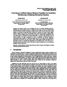
where n is the number of responses, Kn is the weight of the process responses, yd is the desired process response, and yo is the process output resulting from the current input parameters. Values of F near unity indicate high degrees of fitness. Once the individuals have reproduced, they are stored in a “mating pool” awaiting the genetic manipulation process. As the population evolves through reproduction and genetic manipulation, each generation is increasingly capable of solving the problem. In general, the GAs operate through a cycle of four stages: (1) creation of a “population” of strings; (2) evaluation of each string; (3) selection of “best” strings; and (4) genetic manipulation to create a new population of strings. The genetic reproduction process combines chromosomes from one generation and produces new chromosomes that maintain the best features of the previous generation. The most common methods for recombination are crossover and mutation. The crossover operator takes two randomly selected chromosomes and interchanges part of their genetic information to produce two new chromosomes. The crossover point is randomly chosen, and portions of the parent strings are swapped to produce new offspring based upon a specified crossover probability. Mutation is motivated by the possibility that the initially defined population may not contain all the information necessary to solve the problem. This operation is implemented by randomly changing a fixed number of bits every generation based upon a specified mutation probability. Typical values of the probabilities of crossover and mutation range from 0.6 to 0.9 and 0.001 to 0.03, respectively. When GAs and neural networks are combined for process optimization, GAs produce the proposed process inputs for the neural network models. The neural networks then calculate predicted responses, and their output is provided to the GA until a suitable stopping criterion, such as a maximum number of generations or a user defined minimum error, is achieved. The weighting coefficients for the desired responses (see Eq. 4) must also be determined. Figure 3 illustrates the process optimization procedure for a combined GA and neural network implementation.
Desired Response
Genetic Optimizer
Process Set Points
Neural Network Model Figure 3 – Process optimization procedure.
4.
OBORNNS
The Object-Oriented Neural Network Simulator (ObOrNNS) allows users to create, train, and exercise neural networks for the purpose of designing empirical and semiempirical models of semiconductor manufacturing processes, as well as optimizing processes based on those models. Using this program, networks are trained with experimental data that span the ranges the process conditions of interest and are subsequently tested on the remaining data that was not introduced during training. Training is considered complete when the RMSE of the network output is below a user-defined tolerance. While the previous C++ version of ObOrNNS used a command line for input to the software, the updated Java version has a user-friendly graphical user interface (GUI). The use of Java makes the program platform-independent, allowing for access to different types of operating systems, including Windows, Unix, Macintosh.
4.1. ObOrNNS Features ObOrNNS employs a “madaline” architecture with no input bias for forward propagation. Any size neural network with any number of hidden layers and neurons per layer can be used. The networks are limited only by the resources of the operating system. The standard BP algorithm is used for network training. The hyperbolic tangent is used as the default activation function, but the exponential sigmoid activation function is also an option. The program was developed in such a way that additional activation functions can be implemented easily using plug-ins. The user can define the learning rate and/or momentum constant. The user also has the option of training the network by vector or epoch. When training by vector, the weights of the network are updated after each vector is introduced to the network. When training by epoch, the network weights are updated by an average of the errors between the target and network output after all input vectors have been introduced for one epoch. The network can be created with random weights or weights loaded from a file. The weights loaded from a file are usually saved from a previous training session. Training and test data can also be loaded from a file. Figure 4 illustrates the object hierarchy implemented in this ObOrNNS. The classes that simulate the neural network structure are Network, Layer, Neuron, and Weight. The Layer class implements generic neural layers and is extended by two specializations: InputLayer and OutputLayer. The Neuron class provides the structure of a single neuron, and it is extended by three specializations: InputNeuron, BiasNeuron, and OutputNeuron. The Weight class provides the structure for the weighted interconnections between the layers. The Network class implements the Layer class. The Layer class implements the Neuron class, and the Neuron class implements the Weight class.
shuffling data vectors during training, saving networks, and testing networks. The structure of the network is listed in the title of the window in parentheses.
Figure 4 – ObOrNNS programming structure. The portion of the program that implements the neural network and manages the training algorithm and settings is the NetworkManager class. This super-class creates and manages a network by implementing the following subclasses: ActivationFunction, TrainingSettings, Trainer, Network, and WeightSettings. The ActivationFucntion class is an abstraction that allows customization of the nonlinear transfer function for neural output calculation. This class can be extended to allow alternate calculations to be implemented via plug-ins. The TrainingSettings class determines how the network is trained, while the Trainer is an abstraction that allows different training algorithms to be implemented via plug-ins. ObOrNNS provides two standard training algorithms (train-by-epoch and train-byvector) via the EpochTrainer and the VectorTrainer plug-ins. The WeightSettings class passes the values of the learning rate and momentum to the weights. The NetworkManager also does data management and uses the training set to create a scale for the input and output data. The input data is scaled from -1 to 1 while the output data is scaled form –0.5 to 0.5.
4.2. Running ObOrNNS ObOrNNS is available for any platform that supports a Java virtual machine (VM). If the computer does not have the Java VM, it must be installed (can be downloaded from http://java.sun.com) to run the program. The Java version of ObOrNNS is significantly faster in training than all previous C/C++ versions. This is likely due to the new object structure and better interface of the current version. However, the startup time is slightly longer because the Java VM and the GUI components have to be loaded. Nonetheless, once the GUI is up and running, the user can create, modify, test, and save multiple networks in a much friendlier environment (in separate windows) compared to the previous version of the program. At the main menu, networks can be created or loaded to the program. To create a network, the user must specify the structure of the feed-forward network by providing the number of layers and the number of neurons in each layer. There must be at least three layers in a network. The first layer is considered the input layer, while, the last layer is the output layer. After a network is created or loaded, the user is presented with the “Network Browser” interface (see Figure 5), where the user can view the network structure and select training parameters for the network. These parameters include: selecting datasets, activation functions, learning rate, momentum, and training error (scaled value), randomizing network weight,
Figure 5 – ObOrNNS graphical user interface.
4.3. Training Networks Networks are trained by pressing the “Train” button, which initiates the training loop for the network. When “Train” is pressed, a status bar depicts the number of training iterations, and a second status bar depicts the current RMSE in relation to the target. Training will stop either when the “Stop” button is pressed or when one of the other terminating conditions has been reached. When training is stopped by the user, the user may change settings and press “Retrain” to continue training the network from where it was stopped. However, the number of iterations and current RMSE are reset. If training is stopped due to either of the terminating conditions being reached, the network will automatically lock the settings to prevent accidental modifications of the settings. To change the settings, the user must uncheck the “Lock” checkbox. In the testing area of the “Network Browser,” the “Test,” “Dataset,” “Vector,” and “Keyboard” selectors are present. In this area, the users can test a trained network. After a test dataset is loaded and selected, the user can test the entire dataset, one vector in the dataset, or a vector input from the keyboard. After the network output is displayed, it can be saved to a text file by pressing “Save”. Both datasets for testing and training a network are automatically scaled to [-1, 1] and [-0.5, 0.5], respectively, once the “Train” or “Test” buttons are pressed.
5.
APPLICATIONS
5.1. Empirical Modeling of RIE In a purely empirical example of semiconductor process modeling, ObOrNNs was used to model the reactive ion etching (RIE) of benzocyclobutene in a SF6/O2 plasma. The following responses were simultaneously considered: etch rate, uniformity, selectivity and anisotropy. Data for modeling was obtained from a 24 factorial experiment with three center point replicationss designed to characterize etch process variation with respect to the two gas flows, RF power and chamber pressure. This experiment was further augmented with a central composite circumscribed design [24]. The prediction RMSE was less than 16%. Figure 6 illustrates the response surface of the etch rate as a function of SF6 and O2 flow rates.
-6
Anion Exchange - As4=4x10 Torr Phosphorus Composition y
25
Predicted Composition (%)
22.5 20 17.5 15 12.5 10 7.5 5 2.5 0 0
Figure 6 – Response surface for an empirical RIE model.
2.5
5
7.5
10 12.5 15 17.5 20 22.5 25
Measured Composition (%)
5.2. Semi-Empirical Modeling of MBE
Training Data
ObOrNNs also implements semi-empirical modeling by allowing analytical physical models to be incorporated within a neural network framework via a Java plug-in interface [25]. This technique has been used to develop a hybrid neural network model of the growth kinetics of anion exchange in molecular beam epitaxy (MBE). The model was constructed by characterizing the MBE growth of mixed arsenic/phosphorus III-V heterostructures using a D-optimal experiment. The phosphorus composition at the interfaces of these structures was modeled as a function of substrate temperature, phosphorus exposure time, and arsenic stabilizing flux. The semi-empirical model incorporates a kinetic model with a neural network. The kinetic model describes the physical interactions of the processes occurring at the interface, while the neural network estimates the following unknown process parameters: the sticking coefficient (s), desorption coefficient and its associated activation energy (τ0d, Ed), and diffusion coefficient and its activation energy (D0, Ea). Network training occurs using a modified error gradient that takes into account the error contribution from each kinetic parameter determined by the partial derivatives of the kinetic model (see Figure 7). The parameter values obtained using the hybrid approach were s = 0.358 cm2, τ0d = 6.41 sec, Ed = 2.99 eV, D0 = 7×10-15 cm2/sec and Ea = 0.107 eV. Using these estimated parameters, the kinetic model predicts the phosphorus composition of the mixed arsenic/phosphorus III-V heterostructures with a prediction RMSE of less than 1%. Figure 8 illustrates the measured composition versus the predicted composition indicating the accuracy of the hybrid neural process model.
Test Data
Figure 8 – Predicted versus measured composition for semiempirical MBE model.
5.3. Recipe synthesis of PECVD To illustrate its recipe synthesis capabilities, ObOrNNs was used to empirically model plasma-enhanced chemical vapor deposition (PECVD) of silicon dioxide [26]. The PECVD model was subsequently used for optimization via genetic algorithms, which are implemented as another feature in ObOrNNS. Using this approach, appropriate input conditions to achieve desirable film properties are determined. Two important film parameters, deposition rate and uniformity, were first modeled using neural networks. The process conditions subsequently optimized were substrate temperature, pressure, RF power, SiH4 flow, and N2O flow. Using a factorial experiment, the levels of these five process conditions were varied, and the data collected was used for neural network training. The PECVD model for deposition rate and non-uniformity exhibits a prediction error less than 6%. Table 1 shows the optimum recipe for combined target responses of 100% uniformity and maximum deposition rate. These results have been verified experimentally [12]. The discrepancy between simulated and measured response stem from any combination of several possible sources of error In order of decreasing significance, these error sources are: (1) PECVD equipment error; (2) measurement error; (3) human error; (4) model error [12]. Table 1. Optimization Results for PECVD of SiO2
Kinetic Parameters
Growth Conditions P2 flux Ts texp As flux ya
Neural Network
s τ0d Ed D0 Ea
Predicted Composition
Kinetic Model
% Uniformity SiH4 (sscm) N2O (sscm) Temperature (C) Pressure (torr) RF Power (watts) Simulation Results
yp
Back-Propagation
Experimental Composition
Figure 7 – Structural implementation of the hybrid neural network capable of estimating the kinetic parameters.
6.
100.00
Deposition Rate 245 618 197 1.46 83 455 (A/min)
CONCLUSIONS
A general-purpose, object-oriented neural network simulation package has been developed to model and optimize semiconductor processes. Since ObOrNNS was developed in Java, it is platform-independent and can be used on most
operating systems. Using the error-back-propagation training algorithm, ObOrNNS modeling yields excellent results, and the Java implementation enables ObOrNNS to be customized to various purposes with minimum effort. For example, ObOrNNS allows the implementation of hybrid neural networks for semiempirical modeling and parameter prediction, and a genetic algorithm feature provides the capability of recipe synthesis using trained neural network models. In addition, ObOrNNS can conceivably be used for real-time control of semiconductor fabrication equipment. By integrating process modeling, optimization, and control, ObOrNNS can contribute to the success of semiconductor manufacturing in an automated and efficient fashion.
ACKNOWLEDGMENT The authors wish to thank the National Science Foundation, the Packaging Research Center, and the Microelectronics Research Center at the Georgia Institute of Technology for support of this research.
REFERENCES [1] G. S. May, “Manufacturing ICs the Neural Way,” IEEE Spectrum, September 1994, pp. 47-51. [2] G. May, “Application of Neural Networks in Semiconductor Manufacturing Processes, “Chapter 18 in Fuzzy Logic and Neural Network Handbook, (C.H. Chen, Ed.), New York: ASME Press, 1996. [3] B. Kim and G. May, “Reactive Ion Etch Modeling using Neural Networks and Simulated Annealing,” IEEE Transactions on Semiconductor Manufacturing, Vol. 19, No. 1, 1996, pp. 3-8. [4] S. Hong and G. May, “Neural Network Based Time Series Modeling of Optical Emission Spectroscopy Data for Fault Detection in Reactive Ion Etching,” Proceedings of the SPIE Conference on Advance Microelectronic Manufacturing, Vol. 5041, February, 2003, pp. 1-8. [5] R. Pratap, S. Pinel, D. Staiculescu, J. Laskar, and G. May, “A Neural Network Model for Sensitivity Analysis of Circuit Parameters for Flip Chip Interconnects,” Proceedings of the Electronic Components and Technology Conference, 2003, pp. 1619-1625. [6] C. D. Himmel, and G. S. May, “Advantages of Plasma Etch Modeling Using Neural Networks Over Statistical Techniques,” IEEE Transactions on Semiconductor Manufacturing, Vol. 6, No. 2, May 1993, pp. 103-111. [7] C. Davis, R. Tanikella, P. Kohl, and G. May, “Neural Network Modeling of Variable Frequency Microwave Curing,” Proceedings of the Electronic Components and Technology Conference, 2002 pp. 931–935. [8] C. Davis, R. Tanikella, T. Sung, P. Kohl, and G. May, “Optimization of Variable Frequency Microwave Curing using Neural Networks and Genetic Algorithms,” Proceedings of the Electronic Components and Technology Conference, 2003, pp. 1718–1723. [9] T. Thongvigitmanee, and G. S. May, “Optimization of Nanocomposite Integral Capacitor Fabrication Using Neural Networks and Genetic Algorithms,” 27th Annual IEEE/SEMI International Electronics Manufacturing Technology Symposium, July 17 - 18, 2002, pp. 123-129. [10] S. Han, L. Cai, G. May, and A. Rohatgi, “Optimizing the Growth of PECVD Silicon Nitride Films for Solar Cell Applications using Neural Networks and Genetic Algorithms,” Intelligent Engineering Systems Through Artificial Neural Networks, Vol. 6, (C.H. Dagli, Ed.), New York: ASME Press, 1996, pp.343-349.
[11] S. S. Han, “Modeling and Optimization of Plasma Enhanced Chemical Vapor Deposition using Neural Networks and Genetic Algorithms.” PhD Dissertation, the Georgia Institute of Technology, September 1996. [12] S. Han and G. May, "Using Neural Network Process Models to Perform PECVD Silicon Dioxide Recipe Synthesis via Genetic Algorithms," IEEE Transactions on Semiconductor Manufacturing, Vol. 10, No. 2, May, 1997, pp. 279-287. [13] D. Stokes, and G. May, “Real-Time Control of Reactive Ion Etching Using Neural Networks,” IEEE Transactions on Semiconductor Manufacturing, Vol. 13, No. 4, November 2000, pp. 469-480. [14] T. S. Kim and G. May, “Intelligent Control of Via Formation Process in MCM-L/D Substrate Using Neural Networks,” 1999 International Symposium on Advance Packaging Materials, 1999, pp. 106-112. [15] B. Kim and G. S. May, “Real-Time Diagnosis of Semiconductor Manufacturing Equipment Using Neural Networks,” IEEE/CPMT International Electronics Manufacturing Symposium, 1995 pp. 224-231. [16] http://www.calsci.com/index.html [17] http://www.mathworks.com/products/neuralnet/ [18] http://www.neuralware.com/ [19] http://www.neurosolutions.com/ or http://www.nd.com/ [20] http://www.iau.dtu.dk/research/control/nnsysid.html [21] L. Fausett, Fundamentals of Neural Networks: Architectures, Algorithms, and Applications, PrenticeHall, Inc. 1994. [22] D. Goldberg, Genetic Algorithms in Search, Optimization, and Machine Learning, Reading, MA: Addison-Wesley, 1989. [23] J. F. Frenzel, “Genetic Algorithms: A new breed of optimization,” IEEE Potentials, Vol. 12. No. 3, 1993, pp. 21-24. [24] S. Hong, G. May, and D. Park, "Neural Network Modeling of Reactive Ion Etching Using Optical Emission Spectroscopy Data," IEEE Transactions on Semiconductor Manufacturing, Vol. 16, No. 4, November 2003, pp. 598-608. [25] Z. Nami, O. Misman, A. Erbil and G. May, "SemiEmpirical Neural Network Modeling of Metal-Organic Chemical Vapor Deposition," IEEE Transactions on Semiconductor Manufacturing, Vol. 10, No. 2, May, 1997, pp. 288-294.